Revisiting the Parallax of the Isolated Neutron Star RX J185635-3754 Using HST/ACS Imaging

Abstract

We have redetermined the parallax and proper motion of the nearby isolated neutron star RX J185635-3754. We used eight observations with the high resolution camera of the HST/ACS taken from 2002 through 2004. We performed the astrometric fitting using five independent methods, all of which yielded consistent results. The mean estimate of the distance is 123${}^{+11}_{-15}$ pc ($1~{}\sigma$), in good agreement with our earlier published determination.

1 Introduction

Distance is one of the most fundamental attributes of an astrophysical source. The conversion of most observable quantities (e.g., flux, angular diameter, proper motion) to invariate physical units (e.g., luminosity, linear diameter, space velocity) depends the distance to some power. The distance can be determined in a model-independent manner using the trigonometric parallax $\Pi$. This geometrical measure of the distance is one of the most demanding measurements in all of astrophysics because the angles involved are so small.

Here we revisit the distance to the isolated neutron star RX J185635-3754. This object is one of the so-called “Magnificent 7” (Haberl, 2007), a collection of thermally-emitting isolated compact objects. These objects are of interest because, in principle, we can estimate their angular radii from the observed flux and atmospheric models. Measurement of the radius is a necessary step in determining the mass-radius relation for neutron stars (if indeed they are neutron stars and not some more exotic object) and constraining the equation of state of matter at nuclear densities (Lattimer & Prakash, 2001).

Because these isolated stars neither accrete from a binary companion nor have spectra dominated by non-thermal emission, they afford our best opportunity to examine the surfaces of neutron stars. If the mass can also be estimated, say, from a gravitational redshift, then within the uncertainties one can tightly constrain the nuclear equation of state. Even without a mass constraint, an accurate radius measurement (to within 10%) is sufficient to constrain significant, and to date uncertain, nuclear matter properties such as the density dependence of the nuclear symmetry energy.

The population of isolated neutron stars consists of objects that are still sufficiently young ($\lesssim 10^{6}$ years) that the thermal emission from their surfaces is detectable in soft X-rays. Older objects both cool (shifting the emission into the largely unobservable EUV) and fade. In the optical these young objects have absolute magnitudes of about 20. By an age of a few million years, an X-ray-bright isolated neutron star with a heavy element surface will have cooled from 10⁶K to 10⁵K, with a corresponding 10 magnitude decrease in brightness (Page et al., 2004).

The isolated, radio-quiet, thermally-emitting soft X-ray source RX J185635-3754 was discovered by Walter et al. (1996). The optical counterpart, identified by Walter & Matthews (1997), is a blue point source with V$\sim$25.7. Unlike the other members of the Magnificent 7, there is no evidence for any absorption features in the X-ray spectrum. There must be surface inhomogeneities, however, as the object has been seen to rotate with a 7 second period (Tiengo & Mereghetti, 2007). The magnetic field is inferred to be of order 10¹³G (van Kerkwijk & Kaplan, 2008), based on a very uncertain measurement of the spindown. While the X-ray spectrum is indistinguishable from black body with kT_∞=63 eV (Burwitz et al., 2003), and the UV/optical spectral energy is consistent with the Rayleigh-Jeans tail of a hot (T${}_{\infty}>6.5$ eV) black body (Pons et al., 2001), the two spectra do not match. The long wavelength flux is about a factor of 7 larger than an extrapolation of the X-ray blackbody into the optical. Aside from the lack of any features in the X-ray spectrum, these properties are similar to those of the other members of this small class of isolated neutron stars.

A number of lines of reasoning point to RX J185635-3754’s being a nearby compact object. Perhaps the most compelling is that the measured interstellar extinction is small, yet the line of sight passes near the Corona Australis star forming region and its associated molecular clouds, which are at a distance of about 120–140 pc (Maracco & Rydgren, 1981; Neuhäuser & Forbrich, 2008). Because this distance is amenable to direct measurement, and because of the fundamental importance of constraining the equation of state at nuclear densities, we set out to measure the parallax of this object.

Walter (2001) published a parallax of 16.5$\pm$2.3 milli-arcsec (mas), which corersponds to a distance of 61 pc, based on 3 HST/WFPC2 images. This was later found to be erroneous. Kaplan et al. (2002) published a parallax of 7$\pm$2 mas (140 pc). After incorporating a fourth WFPC2 image, Walter & Lattimer (2002) reported a revised parallax of 8.5$\pm$0.9 mas (117$\pm$12 pc). Based on models of the interstellar extinction, Posselt et al. (2007) find likely distances between 125 and 135 pc.

The radius of the neutron star is the product of the model-dependent angular radius and the distance. The simplest models, blackbody fits to the X-ray spectrum, yield unrealistically small radii of a few km, and ignore information contained in the longer wavelength spectra. The isolated neutron stars have optical excesses relative to their X-ray fluxes (e.g., Pons et al. 2001, Haberl 2007); models that have been considered to explain the spectrum include two-component black bodies, a condensed magnetized heavy element surface (Pérez et al., 2005), and optically thin partially-ionized hydrogen atop a condensed surface (Ho et al., 2007). Walter & Lattimer (2002) fit a simple two-blackbody model. They showed that at 117 pc, the radiation radius R_∞ is $<$26 km (it depends on the ill-defined temperature of the cooler component), with a formal best-fit radius of 16.4$\pm$1.7 km, where the uncertainty reflects that of the distance. Trümper et al. (2003) find a conservative lower limit to the radius of 16.5 km for a two blackbody fit at the same distance. Ho et al. (2007) fit their magnetic H-atmosphere plus condensed surface model, and find R_∞=17 km, assuming a distance of 140 pc (14 km at a distance of 117 pc).

Seeing a need to confirm this measurement, Kaplan et al. re-observed the target with the High Resolution Camera (HRC) of the Advanced Camera for Surveys (ACS) on the Hubble Space Telescope. The factor of two improvement in plate scale affords the opportunity to refine the measurement, reduce the uncertainty in the distance, and yield improved physical parameters for the closest isolated neutron star. Kaplan et al. (2007) and van Kerkwijk & Kaplan (2007) reported distances of 167${}^{+18}_{-15}$ pc and 161${}^{+18}_{-14}$ pc, respectively, without providing details.

In this paper we analyze these ACS/HRC images to measure the parallax of RX J185635-3754 at a second epoch.

2 Observations

The target was observed with the ACS/HRC on eight occasions over a 20 month span, beginning in 2002 September (Table 1). The HST program ID is 9364; the PI is D.L. Kaplan.

There are two requirements for astrometric observations: a large plate scale because the motions are small, and a large field of view, to maximize the number of background reference objects. The HRC channel of the ACS is a 1024$\times$1024 pixel CCD camera with a nominal pixel size of about 28 milli-arcsec. It was presumably selected for these observations because of the large plate scale. The relatively small field of view and commensurately small number of potential reference stars is the main limitation on the accuracy with which the images can be coaligned, or transformed, to a common reference frame.

At each visit four observations were taken using the standard 4-point dither pattern with 2.5 pixel offsets in each coordinate. Each integration was 620 seconds through the F475W filter. Images were not CR-SPLIT.

All observations were obtained in Fine Lock mode. There were no guiding anomalies. The RMS jitter varies between 1.4 and 3.4 mas. While some of the JIF images show minor elongation of the psf, this will not affect the positional measurements.

The visits were scheduled $\pm$ 1 month from the extrema of the parallactic displacement in right ascension. At the ecliptic latitude of the target, the position angle of the ellipse is 83^∘ with an aspect ratio of about 5:1. Consequently the parallax is better detectable in residuals in right ascension than in declination.

2.1 Methodology

We measure the residual motions of the target differentially, with respect to the other stars in the images. We assume that there is no bulk motion of the other stars – that is, the directions of the proper motions of the reference stars are randomly directed. In the pathological case that all the reference stars are members of a moving group, with a shared proper motion and identical parallaxes, then the method of differential astrometry would fail as the shared motions would be interpreted as detector offsets. There is no evidence that this is the case. Note that a bulk motion will only affect the derived proper motions. We show later that the reference stars in this field are at distances $>$10 kpc, so the correction from relative to absolute parallaxes must be small.

Because the parallax is small – a fraction of a pixel in size – we need to take great care with the reductions. Therefore, we decided that each of the investigators would analyze the data independently, using different fitting techniques. We started from a common set of processed images.

2.1.1 Initial Data Processing

The initial data processing consists of cleaning the images of cosmic rays, and correcting the pixel positions for distortions in the detector.

Cosmic rays are a problem with all CCD detectors. While largely cosmetic, occasionally a cosmic ray does hit within the point spread function of a source, and will affect both the astrometry and the photometry. We begin with the flat-fielded _flt.fits images. We reject all pixels with a data quality flag set to 2048 or greater (those identified as saturated pixels and cosmic rays) by setting the data value equal to the median of the surrounding 8 pixels. About 2% of the pixels in each image are so-affected. This is mostly done to simplify the data reduction code, where large data values can draw off a mean or median. But in the end this is of little consequence. We save this cosmetically-corrected image as a fits file.

The ACS is a radial bay instrument on the HST, hence there is significant and asymmetric distortion in the images (Anderson & King, 2004). We use Anderson’s img2xym_HRC Fortran code to find the stars in the cosmetically-corrected images and to correct for the instrumental distortion. This code determines positions by doing a PSF-fit using the filter-specific point spread function. According to Anderson & King (2004), the distortion correction corrects to better than 0.01 pixel in each coordinate for sufficiently bright stars. The output of this code is a list of raw and corrected X and Y positions in the instrumental frame, along with an instrumental magnitude. The code does not return any estimate of the uncertainty in the position. We adopt the mean pixel scale of 0.02827 arcsec/pix.

Using the thresholds we selected (HMIN=5, FMIN=150), we identify 21 stars in the field that are common to at least five of the visits, in additional to the neutron star. Thirteen of these stars are recovered in all visits, and five are seen in seven of the visits. The others lie close enough to edge of the detector that instrumental rotation leaves them outside the field of view on occasion. Only the fifth visit contains all 21 stars.

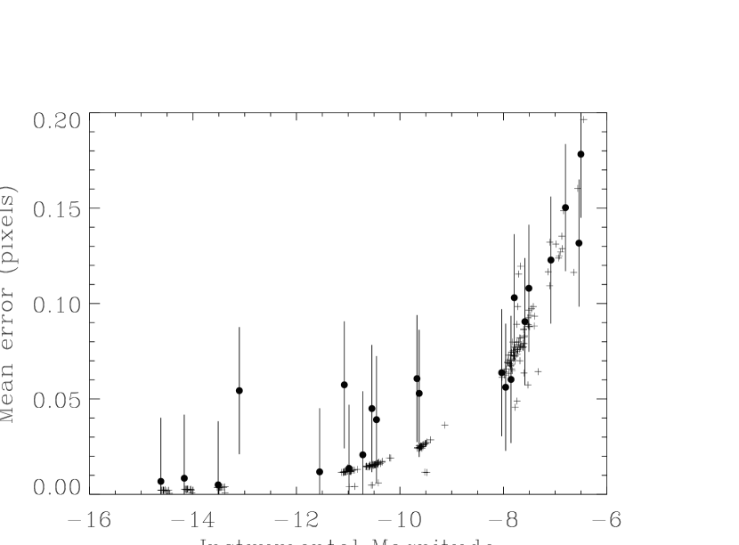
Figure 1: The median uncertainty in the accuracy of the transformations as a function of instrumental magnitude (solid circles). The uncertainty is computed as the scatter in the position after transformation at each epoch. There is a single uncertainty for each star at each epoch, hence 8 points contribute to the median. The small + symbols are the formal uncertainties on the positions, as measured using the IDL starfinder procedure.

We estimate the measurement uncertainties $\sigma$ at each iteration of the various fits. We take the measurement error on a particular star to be the standard deviation of the position measurements in the 4 images obtained during a visit after transforming to a common frame. As the transformation changes, so do these uncertainties. Where a positional measurement disagrees by more than one pixel from the mean of the other three, we flag that measurement as bad and ignore it. Most such instances are due to cosmic rays affecting the initial PSF fit. The uncertainties $\sigma$ vary from star to star and for each visit, but are identical for the 4 measurements of a star in a particular visit. We set a minimum $\sigma$=0.01 pix, the accuracy to which Anderson & King (2004) claim to be able to measure the positions. As expected, $\sigma$ increases with instrumental magnitude (Figure 1. In this plot we also show the formal uncertainties on the positions as extracted using the IDL StarFinder procedure (Diolaiti et al., 2000). The two agree well.

The initial transformations are accomplished by first shifting the measured positions within a given visit by the nominal dither, and then rotating the X,Y coordinates of the stars to nominal north using the ORIENTAT keyword in the fits images. We wrote four independent $\chi^{2}$ minimization astrometric fitting codes, and wrote another incorporating the IDL function MPFITFUN. Our fitting codes differ in small details, including how they solve for the parallax ellipse, how they reject outliers, and how they estimate the measurement uncertainties. We refer to these models as A1 through A4 in Table 3. As a test, we also fit the data using a publicly-available astrometric package, ATPa (model T). Finally, we generated an independent Bayesian estimate of the parallax and proper motion (referred to as model B). The various models yielded indistinguishable results.

2.1.2 Astrometric Fitting by $\chi^{2}$ Minimization

This is a general description of astrometric fitting via $\chi^{2}$ minimization. In detail this corresponds to model A1. Differences between the models are described below. Our notation is such that $i$ refers to a star, $k$ refers to an epoch, and $j$ refers to one of the four images at that epoch. There are a total of $JK=32$ images and $I=21$ field stars.

We register all images by solving for their centers and relative rotations. The plate scale is not necessarily the same for all images. We considered the case where the scale varied independently in the X and Y directions, but found no need for this. We limited our fitting to a scalar scale change. The stars have proper motion and a correction for parallax might need to be included.

The measured positions form the data sets $x_{i,j,k}$ and $y_{i,j,k}$. If the positions of all field stars appeared on all frames there would be a total of 672 $(x,y)$ points, but the positions of some stars on some frames are invalid, either because they fall off the frame, or because they exceed the 1 pixel error tolerance we adopted.

The function to be minimized is

$$\chi^{2}=\sum_{i,j\neq 0,k\neq 0}\left[{(X_{i,j,k}-x_{i,j,k})^{2}\over\sigma_{x,i,j,0}^{2}+\sigma_{x,i,j,k}^{2}}+{(Y_{i,j,k}-y_{i,j,k})^{2}\over\sigma_{y,i,j,0}^{2}+\sigma_{y,i,j,k}^{2}}\right]$$ (1)

where the sum is over the valid indices. The model predictions for the positions, relative to a reference position $(x_{i,0,0},y_{i,0,0})$, are

$$\begin{array}[]{ll}X_{i,j,k}=M_{j,k}[\cos(\theta_{j,k})x_{i,0,0}-\sin(\theta_{j,k})y_{i,0,0}+\Delta x_{j,k}+\mu_{x,i}t_{k}+P_{x,k}\Pi_{i}],\\ Y_{i,j,k}=M_{j,k}[\cos(\theta_{j,k})y_{i,0,0}+\sin(\theta_{j,k})x_{i,0,0}+\Delta y_{j,k}+\mu_{y,i}t_{k}+P_{y,k}\Pi_{i}].\end{array}$$ (2)

The reference position is taken to be the first frame ($j=0$) of either the first or fifth epochs ($k=0$ or 4) except when the stellar data for that frame is invalid, in which case the next frame of the epoch is used. In all cases, we use the notation $0,0$ to refer to the reference image. $M$ refers to the plate’s relative scale factor, or magnification, $\theta$ to the plate’s relative rotation, $\mu_{x}$ and $\mu_{y}$ to the star’s proper motion, $t$ to the difference in epoch between an image and the reference image, and $\Pi=1/D$ where $D$ is the stellar distance. $P_{x}$ and $P_{y}$ are the relative parallactic displacements which depend on the time of year. If the parallax $\Pi$ is in units of pc^-1, then $P_{x}$ and $P_{y}$ have units of pixels-pc. With these definitions $M_{0,0}=1$, $\Delta x_{0,0}=\Delta y_{0,0}=\theta_{0,0}=t_{0}=P_{x,0}=P_{y,0}=0$. It follows that $X_{i,0,0}=x_{i,0,0}$ and $Y_{i,0,0}=y_{i,0,0}$. Initially, it is assumed $\mu_{x,i}=\mu_{y,i}=\Pi_{i}=0$ for all $i$.

The measurement errors, $\sigma_{x,i,k}$ and $\sigma_{y,i,k}$, are the standard deviations among the measured positions for each star at each epoch, which normally numbers $J_{i,k}=4$.

$$\begin{array}[]{ll}\sigma_{x,i,k}=\sqrt{\sum_{j}(X_{i,j,k}-x_{i,j,k})^{2}/J_{i,k}},\\ \sigma_{y,i,k}=\sqrt{\sum_{j}(Y_{i,j,k}-y_{i,j,k})^{2}/J_{i,k}}\end{array}$$ (3)

These errors are same for all values of $j$ for each value of $k$. As discussed above, we set a floor of 0.01 pix as the minimum value for $\sigma$.

The plate registration is done in the standard way by solving the $4(JK-1)=124$ simultaneous equations for the minimization of $\chi^{2}$:

$$\begin{array}[]{llll}{\partial\chi^{2}\over\partial\Delta x_{j,k}}=0,\\ {\partial\chi^{2}\over\partial\Delta y_{j,k}}=0,\\ {\partial\chi^{2}\over\partial\theta_{j,k}}=0,\\ {\partial\chi^{2}\over\partial M_{j,k}}=0.\end{array}$$ (4)

Note that in these equations, $(j,k)\neq(0,0)$.

We use a Newton-Raphson approach to solving the set of equations $f_{i}(x_{j})=0$. Assume an initial guess $x_{0j}$ and make the Taylor expansion to determine the corrections $dx_{0j}$:

$$f_{i}(x_{0j})+{\partial f_{i}\over\partial x_{j}}dx_{0j}=f_{0i}+A_{ij}dx_{0j}=0.$$ (5)

Solving this system gives $dx_{0j}=-(A_{ij})^{-1}f_{0i}.$ The new guess becomes $x_{1j}=x_{0j}+dx_{0j}$, a new Taylor expansion is made, and a new correction $dx_{1j}$ is estimated and so forth until convergence is achieved.

Next, the stellar parameters, their proper motions and distances, are determined from the $3I=63$ simultaneous equations

$$\begin{array}[]{lll}{\partial\chi^{2}\over\partial\mu_{x,i}}=0,\\ {\partial\chi^{2}\over\partial\mu_{y,i}}=0,\\ {\partial\chi^{2}\over\partial\Pi_{i}}=0.\end{array}$$ (6)

Now using the non-zero values for $\mu_{x,i},\mu_{y,i}$ and $\Pi_{i}$, the positional errors and plate registrations are repeated. The scheme converges after about 4 iterations.

The target star parameters are established once convergence is achieved by minimizing

$$\chi^{2}_{\rm NS}=\sum_{j,k}\left[{(X_{{\rm NS},j,k}-x_{{\rm NS},j,k})^{2}\over\sigma_{x,{\rm NS},j,0}^{2}+\sigma_{x,{\rm NS},j,k}^{2}}+{(Y_{{\rm NS},j,k}-y_{{\rm NS},j,k})^{2}\over\sigma_{y,{\rm NS},j,0}^{2}+\sigma_{y,{\rm NS},j,k}^{2}}\right],$$ (7)

utilizing the above expressions for $i=NS$ and solving the equations for $i=$NS, where NS is the index corresponding to the neutron star.

2.1.3 Transform Uncertainties

The transformations are based on between 18 and 21 stars in each visit. The median residual error in the transformation (the difference between the modeled stellar positions and the reference positions) is 0.05 pixels; the median measurement error is 0.07 pixels. In principle the accuracy of the transform depends on the instrumental magnitude of the stars used. Examining the spread of errors, it is clear that the 12 stars with instrumental magnitudes $<-9$ exhibited less scatter in the residuals. Including only these bright stars gives a median residual error 0.04 pixels with a median measurement error of 0.02 pixels. However, no systematic uncertainties are introduced by using all the stars in the field, and neither the results nor their uncertainties depend on the choice of reference stars.

2.1.4 Determination of Parallactic Ellipse

We determine the parallactic ellipse using standard formulae (e.g., in the Astronomical Almanac), for the nominal coordinates of the target, $\alpha=18^{\rm h}56^{\rm m}35.11^{\rm s}$ and $\delta=-37^{\circ}54^{\prime}30.5^{\prime\prime}$.

2.1.5 Differences in the models

In model A2 we use only the nine bright reference stars that appeared in all 32 images to determine the image transformations. This model uses an iterative approach wherein the plate transformation is fit with all stellar motions fixed at zero. The proper motion is then estimated as a linear trend in the residuals. This is fit, subtracted, and the plate is re-transformed. This process is repeated until the solution converges. The neutron star is not included in the fit. This approach implicitly assumes that all parallaxes are zero. In the second step the parallax and proper motion are fit to the transformed positions of the neutron star. Finally, this process is repeated using all the stars in the image. No significant parallaxes were found, validating the first assumption.

In model A3 we estimate the individual uncertainties empirically in the $\_$flt images using the IDL xstarfinder procedure (Diolaiti et al., 2000). An empirically determined PSF is fitted to each star in each image, resulting in astrometric uncertainties ranging from $\sim$0.01 pixels for bright objects to $\sim$0.09 pixels for the faintest objects, including the target. We use these uncertainties along with the distortion-corrected positions from the img2xym_HRC output. The first image in the first visit is used as a reference frame. We fit the 19 stars visible in the first image (including the neutron star) and performs a $\chi^{2}$ minimization as described above, fitting the proper motions and parallaxes simultaneously.

Model A4 is based on MPFIT. This model can be run using either some (we selected the brightest 12 stars; those with instrumental magnitudes $<-9$) or all the stars in the field for the determining the transformations. An iterative approach is used, similar to that used in model A2, except that the parallaxes and proper motions are fit simultaneously. Parallaxes can be forced to be zero.

2.1.6 Bayesian Error Estimation (Model B)

We transformed the positions of all stars in the images to the reference frame (the first image of the first visit) allowing for 5 free parameters (translations and scale factors in both in X and Y and orientation). We rejected stars which failed to transform (including the target), leaving a subsample of 12 stars to define the reference frame. We estimated the measurement uncertainties by fitting a straight line to the mean errors of these 12 stars as a function of instrumental magnitude. This differs from the scheme used in the A models.

Thus, having positional measurements and corresponding uncertainties of the target in the common reference of frame, we computed posterior probabilities of the parallax and proper motions of the target (all other parameters are treated as nuisance parameters, which are not of immediate interest but which must be accounted for in the analysis of those parameters which are of interest).

The expected geocentric right ascension and declination $\alpha_{GCRS}(t),\delta_{GCRS}(t)$ of the target at a given epoch $t$ can be expressed in the form:

$$\left\{\begin{array}[]{ll}\alpha_{GCRS}(t)=\alpha_{BCRS}(t_{0})+\Delta\alpha_{1}(t,t_{0},\alpha,\delta,\ mu_{\alpha},\mu_{\delta},\Pi,v_{r})+\Delta\alpha_{2}(t,\alpha,\delta,\Pi)\\ \delta_{GCRS}(t)=\delta_{BCRS}(t_{0})+\Delta\delta_{1}(t,t_{0},\alpha,\delta,\ mu_{\alpha},\mu_{\delta},\Pi,v_{r})+\Delta\delta_{2}(t,\alpha,\delta,\Pi)\\ \end{array}\right.$$ (8)

where $\alpha_{BCRS}(t_{0}),\delta_{BCRS}(t_{0})$ are the barycentric coordinates at a reference time $t_{0}$, the pairs ($\Delta\alpha_{1},\Delta\delta_{1}$) and ($\Delta\alpha_{2},\Delta\delta_{2}$) are the corresponding displacements of the star’s position in the right ascension and declination owing to the spatial motion and parallactic motion of the Earth. $(\mu_{\alpha},\mu_{\delta})$ are the right ascension and declination components of the proper motion, $\Pi$ is the annual parallax and $v_{r}$ is radial velocity.

In principle, those expected positions and actual measured ones in different epochs may differ by some uncertainty $\epsilon_{i}$ owing to the measurements errors plus any real signal in the data that cannot be explained by the model:

$$\left\{\begin{array}[]{ll}\alpha_{GCRS}({\rm expected})=\alpha_{GCRS}({\rm measured})+\epsilon_{\alpha}(t)\\ \delta_{GCRS}({\rm expected})=\delta_{GCRS}({\rm measured})+\epsilon_{\delta}(t)\end{array}\right.$$ (9)

In the absence of detailed knowledge of the effective noise distribution, the most conservative choice of the distribution of positional differences ($\epsilon_{i}$) is a Gaussian and therefore for the likelihood we may write:

$$p(D|M(\theta),I)=\prod_{i=1}^{n_{obs}}\frac{1}{2\pi\epsilon_{i}}\exp\left[-\sum_{i=1}^{n_{obs}}(d_{i}-d_{i}({\rm model})))^{2}/(2\epsilon_{i}^{2})\right],$$ (10)

where by $D(d_{i},i=1,n_{obs})$ we denote either the right ascension or the declination of the target at a given epoch.

Using Bayes theorem we may estimate posterior probabilities of parameters:

$$p(M(\theta)|D,I)=\frac{p(D|M(\theta),I)p(M(\theta),I)}{p(D|I)},$$ (11)

where M($\theta$) is a model with parameters ${\boldmath\theta}(\alpha_{BCRS}(t_{0}),\delta_{BCRS}(t_{0}),\Pi,\mu_{\alpha},\mu_{\delta},V_{r})$, and $p(M(\theta),I)$ the prior probabilities of the considered parameters. $p(D|I)$ serves as the normalization.

We used the flat priors for the proper motions and the uninteresting parameters. For the parallax we used both so-called flat priors and the Jefferys priors. The flat prior is a uniform probability distribution within some reasonable interval. In the Jeffreys prior, formulated as

$$p(\Pi|I)=1/(\Pi*Log[\Pi_{\rm hi}/\Pi_{\rm lo}]),$$ (12)

the probability density is uniform in the logarithm of the parallax ($\Pi_{\rm hi}$ and $\Pi_{\rm lo}$ are the upper and lower bounds of the interval considered for the parallax). Use of this prior is motivated the invariance of conclusions with respect to scale changes in time (Jaynes, 1998). This prior is also form-invariant with respect to reparameterization in terms of distance. That is, an investigator working in terms of distance and using a 1/distance prior will reach the same conclusions as an investigator working in terms of Parallax and using a 1/Parallax prior. This would not be true for a prior of another form, for example, a uniform prior. To the extent that parameterization in terms of Distance and Parallax are both equally “natural”, this form of invariance is desirable. Of course, if the prior range of a parameter is small when expressed as a fraction of the center value, then the conclusions will not differ significantly from those arrived at by assuming a uniform prior.

Since the measurement errors play a crucial role in the estimation of the unknown parameters, we considered three different cases:

i) positional uncertainties are known for each epoch (from scaling the uncertainties as a function of instrumental magnitude, as described above).
ii) positional uncertainties are unknown but are the same at all epochs ($\epsilon_{i}=const\times\sigma$).
iii) positional uncertainties are unknown but are different for different epochs ($\epsilon_{i}=const\times\sigma_{i}$).

2.2 Tests

2.2.1 Plate Scale

We checked the plate scale in the reference image by using 5 stars that are in common with the 2MASS catalog. The mean plate scale is 28.38$\pm$0.53 mas/pixel, where the uncertainty is the standard deviation of the 10 independent measurements. There are 4 stars common with the NOMAD-1 catalog (Zacharias et al., 2005). The mean plate scale is 29.55$\pm$1.3 mas/pix. These are both consistent with the mean plate scale from Anderson & King (2004).

2.2.2 Parallax Check

To test our sensitivity to the small expected parallax, we ran a series of tests wherein we replaced the target with a test star of known parallax and proper motion after transforming the frames. We selected a large proper motion similar to that expected from the target. We applied a Gaussian-distributed error to the position of the test star, and then fit the data in an attempt to recover the known motions. Results are shown in Table 2.

2.2.3 Proper Motion Check

The 8 visits to the field occurred at 4 distinct times of the year, within tolerances of 10 days. On a given date, the parallactic factor is the same for all the stars, so we can assume that any difference in position is attributable solely to proper motion. We determined a mean proper motion for each star from the average of these four measurements for each star in the field. Within the uncertainties, the proper motion of the target is fully consistent with those from the global minimizations.

The mean proper motions for the 21 field stars are $\mu_{\alpha}=-2.4\pm 4.7$, $\mu_{\delta}=0.4\pm 3.0$ milli-arcsec/yr. There is no evidence for systemic motions of the field stars.

2.2.4 Tolerance to Rotation and Magnification

The full fit solves for four global parameters (zero-point translations, rotation, and plate scale). The largest change in plate scale relative to the reference image is 6$\times$10^-5; the largest change in orientation from that of the reference image is 0.0055 degrees (20 arcsec). Neither of these are significant. We also ran the fitting routines for the cases where the rotation or the scale factor were assumed not to change. This did not affect the results significantly.

We also solved for the case where the parallax of the reference stars is fixed at zero. This also had no significant effect on the results.

2.2.5 Publicly Available Astrometry Code

Finally, we ran the positions through a publicly-available astrometry code, ATPa (G. Anglada Escudé 2010, in preparation). This code was developed for use in the Carnegie Astrometric Planet Search.

We de-rotated the positions reported by img2xym_HRC using the nominal orientation, so that the (x,y) axes correspond to ($-$RA, Dec) respectively. We wrote out the coordinates in the correct format to input into the ATPa astrometric solution tool. We used the nominal HRC plate scale. Since the geometric distortions have already been removed, we used calibration rank 1 in ATPa, which corrects for linear offsets, rotations, and magnification changes.

Because this code is still under development, and we ran it as a black box, we use it only as a check that our other codes are producing reasonable results. Results are stated in Table 3 as model T. We do not include the ATPa results in our final parallax determination.

2.3 Results

The results of the realizations of these fitting codes are shown in Table 3. As described above, we ran many realizations of each of these codes, using different reference stars for the transformation, selectively excluding stars or entire visits, and allowing the plate scale and rotation to be either fixed or free parameters. We have chosen to present only the mean of the many realizations for each code. Differences are minor. Individual estimates of distances range from 117 to 128 pc (the $\pm 1~{}\sigma$ ranges encompass 109 to 135 pc).

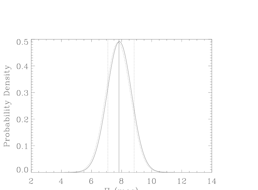
Figure 5: Bayesian posterior probabilities and the estimate of parallax of RX J185635$-$3754. The solid curve is the probability distribution using flat priors; the dotted line is the probability distribution using Jeffreys priors. The 68% credible region centered on the highest probability density for the flat prior solution is enclosed by the vertical dotted lines for case i errors. The probability density is per mas.

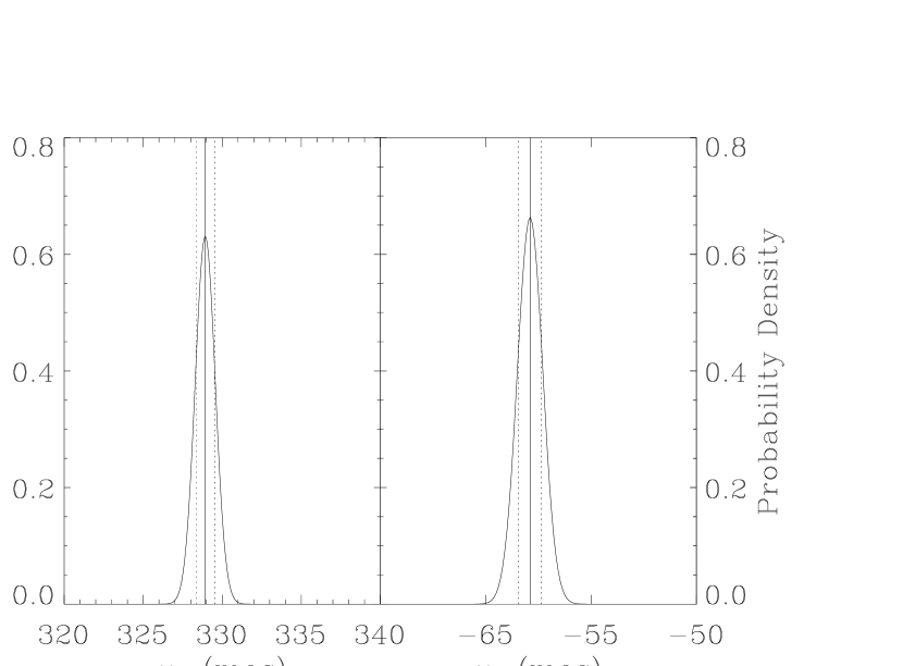
Figure 6: Bayesian posterior probabilities and the estimate of the proper motion in right ascension and declination of RX J185635$-$3754 using the flat prior. The 68% credible region centered on the highest probability density is enclosed by the vertical dotted lines for case i errors. The probability density is per mas.

The parallactic motion in RA and Dec are shown in Figure 3. The full 2-dimensional representation of the parallactic ellipse is shown in Figure 4. The Bayesian estimates for these parameters are shown in Figures 5 and 6. The differences in the Bayesian estimates of the parallax for the two choices of priors, 0.6%, is negligble. The choice of prior for the parallax has ne effect on the proper motion estimate. We use the mean of the two parallax estimates in determing the weighted mean of all the models.

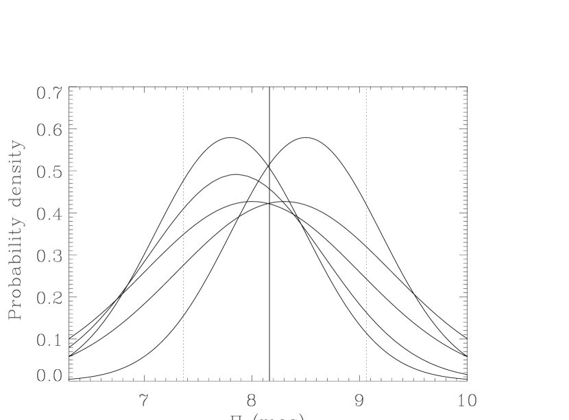
Figure 7: Probability distribution functions for the parallax of RX J185635$-$3754 from the independent astrometric models. The units are probability density per mas. The thick vertical line is the weighted mean, which we adopt as the parallax. The dotted vertical lines encompass our adopted $1~{}\sigma$ confidence region (see text).

It is not clear which, if any, of the codes is to be preferred. The parallaxes of the A and B models all agree to within their $\pm$1 $\sigma$ confidence regions. In the absence of a clear choice, we opt to view these as independent measurements, and take a weighted mean for the final result. From this mean we exclude model T, which we used to corroborate our results. The probability distributions of the independent models are shown in Figure 7.

The five measurements of parallax agree to well within their 1 $\sigma$ uncertainties, with a standard deviation of 0.24 mas. The weighted mean parallax of 8.18 mas corresponds to a distance of 123 pc. Because the 5 measurements all start with the same data, they are not truly independent measurements of data selected from a sample population. Therefore, we adopt the mean error of the individual measurements, 0.8 mas, as representative of the true uncertainty. The corresponding distance is 123${}^{+11}_{-13}$ pc.

Any corrections for systematic errors made by assuming the plate scale and orientation of the reference image are $<6\times 10^{-5}$ and $<\pm 0.0055$ degrees. These are far smaller than our mesasurement errors, and are inconequential.

Note, however, that this is a differential measurement, and that our measured parallax is only a lower limit to the true parallax. Most if not all of the reference objects are likely to be galactic stars. Kaplan et al. (2002) have estimated the distance of the background stars using a $B$ vs. $B-R$ color-magnitude diagram. They conclude that most of the objects are consistent with dwarfs at a distance of order 10 kpc, or K giant members of the Sgr dwarf galaxy at a distance of 25 kpc. The six brightest of our reference objects have $B$ and $R$ magnitudes in the NOMAD-1 catalog; these are consistent with the Kaplan et al. (2002) picture. Star 9 lies near the 25 kpc giant branch; stars 6, 13, 17, and 21 lie near the 10-25 kpc main sequence; star 12 lies about 2 mag below the 25 kpc main sequence. We constructed a color-magnitude diagram using the 10 stars in common between the HRC images and the F606W WFPC2 images (Walter, 2001). We use the 3 of these that also have $B$ and $R$ magnitudes for a crude calibration. If stars 6 and 21 define the 10-25 kpc main sequence (see above), the other 8 stars are 2-3 mag fainter at similar colors. These could main sequence stars at distances of 70-100 kpc (and a galactic scale height of $20-30$ kpc), or white dwarfs at distances of order 10 kpc. We conclude from this crude analysis that the mean absolute parallax of the reference stars is $<$0.1 mas, and that the relative parallax is unlikely to be significantly underestimated. Nonetheless, we will add 0.1 mas to the error budget on the positive side. The consequence is to decrease the lower bound on the distance by about 2 pc. Our best estimate of the distance is 123${}^{+11}_{-15}$ pc.

The $\pm 1~{}\sigma$ confidence region encompasses 108 to 134 pc. This is in good agreement with the previously published value of 117$\pm$12 pc, and with distances estimated from the interstellar extinction. The proper motion (Table 3) compares favorably to that published by Walter & Lattimer (2002).

The F475W magnitude of the neutron star is 25.36$\pm$0.15. This magnitude is the mean of the corrected instrumental magnitudes in each visit from the img2xym_HRC code, converted to apparent magnitude using the photometric zero point for the F475W filter. The uncertainty is the standard deviation of the measurements in the 8 visits. There is no evidence for variability.

As a by-product of this analysis, we have measured magnitudes, proper motions, and parallaxes for the field stars. These are shown in Table 4. Five of the reference stars have proper motions that are formally significant at the 3 $\sigma$ level (one at $>5.0~{}\sigma$), with values ranging from 4 to 14 mas yr^-1. None of the reference stars has a measurable parallax at the $>3~{}\sigma$ level. There is evidence for photometric variability of stars 2 and 21.

3 Discussion

The proper motion and parallax are in excellent agreement with those published earlier by Walter & Lattimer (2002). The proper motions agree at the 0.2% level, and the parallaxes agree to better than 6%, both well within the formal uncertainties. These two measurements were made using different instruments. Their excellent agreement certainly speaks to the great care that has gone into the astrometric calibration of both the HRC (Anderson & King, 2004) and the WFPC2 (Holtzmann et al., 1995), as well as the astrometric stability of the HST as a whole.

That the new HRC results are not superior to the determination from the WFPC2, despite the smaller pixel size of in the HRC, can be attributed to two factors: the smaller plate scale is offset by the larger number of reference stars in the larger WFPC2 field, and the proper motions are better-determined in the WFPC2 images bcause of the longer 4.5 year baseline. Combining these two independent measures results a weighted mean parallax of 8.33$\pm$0.6 mas (120${}^{+8}_{-10}$ pc). A combined analysis of the two data sets is likely to yield vastly reduced errors because the baseline for the proper motion will more than double to 8.5 years. Better-determined proper motions will yield a more accurate transformation, and ultimately a better measure of the parallax.

Obtaining the parallax of this neutron star is only a means to an end. With a distance known to 7%, the largest uncertainty in the radius of this neutron star lies in the atmospheric or surface emission models. In the context of simple two blackbody models the radius R_∞ is 16.8${}^{+1.1}_{-1.4}$ km, where this uncertainty reflcts the statistical uncertainty in the distance (as discussed by Pons et al. (2001), the radius depends critically on the ill-defined temperature of the cool component). The true uncertainty is dominated by systematics in the models. This is still consistent with many equations of state, but combined with information for X-ray bursts and quiescent low-mass X-ray binaries, it can be used to significantly constrain the nuclear equation of state (Steiner et al., 2010).

Figure 2: Motions of RX J1856 after transforming the 32 images to the same reference. The solid curve is the best fit parallax + proper motion; the proper motion and parallactic wobble are clearly evident. The motion is towards the lower left. The dots show the predicted positions at the times of observation. The units are in corrected pixels, 28.27 milli-arcsec. Note that the declination scale is 5 times that of the RA scale.

Figure 3: Residuals to the motion of RX J1856 after subtracting the linear proper motion. The solid curves are the best fit parallactic ellipse; the dotted curves are the 90% confidence regions. The 4 observations at each epoch are not averaged.

Figure 4: Residuals to the motion of RX J1856 after subtracting the linear proper motion. The best fit parallactic ellipse is overplotted. The thick lines represent the mean residual positions at each of the 8 visits, after averaging the 4 individual observations at each visit. The dots are the predicted positions along the parallactic ellipse at the time of observation.

Table 1: Epochs of HRC Exposures.

Start (UT)	Start (MJD)
2002-09-01 04:48:45	52518.201
2002-11-01 08:13:59	52579.343
2003-03-02 02:50:49	52700.119
2003-05-15 22:54:12	52774.954
2003-08-24 16:00:10	52875.667
2003-11-01 00:21:29	52944.015
2004-02-20 21:06:06	53055.879
2004-05-24 19:17:10	53149.804

Table 2: Recovery of Simulated Data.

Input values			Output values			N
$\mu_{x}$	$\mu_{y}$	$\Pi$	$\mu_{x}$	$\mu_{y}$	$\Pi$
mas/yr	mas/yr	arcsec	mas/yr	mas/yr	arcsec
-307.2	51.2	0.0080	-307.3 $\pm$ 1.2	51.5 $\pm$ 1.3	0.0079 $\pm$ 0.0009	2204
-309.8	51.6	0.0060	-309.7 $\pm$ 1.2	52.0 $\pm$ 1.3	0.0069 $\pm$ 0.0010	2001
-309.8	51.6	0.0060	-309.7 $\pm$ 1.2	52.0 $\pm$ 1.3	0.0060 $\pm$ 0.0010	2001
-309.8	51.6	0.0050	-309.7 $\pm$ 1.2	52.0 $\pm$ 1.3	0.0050 $\pm$ 0.0010	2001
-309.8	51.6	0.0040	-309.7 $\pm$ 1.2	52.1 $\pm$ 1.3	0.0040 $\pm$ 0.0010	2001
-309.8	51.6	0.0030	-309.6 $\pm$ 1.2	52.0 $\pm$ 1.3	0.0031 $\pm$ 0.0009	2001
-309.8	51.6	0.0020	-309.5 $\pm$ 1.2	52.0 $\pm$ 1.4	0.0022 $\pm$ 0.0009	2001
-309.8	51.6	0.0010	-309.5 $\pm$ 1.2	52.1 $\pm$ 1.3	0.0011 $\pm$ 0.0009	2001

Table 3: Proper Motion and Parallax Measurements.

Model	$\mu$	PA	$\Pi$	Notes
	(mas/yr)	(deg)	(mas)
A1	332.4 $\pm$0.7	100.8 $\pm$ 0.1	8.5 $\pm$0.7
A2	329.5 $\pm$1.0	100.3 $\pm$ 0.2	8.0 $\pm$1.0
A3	329.3 $\pm$1.0	100.3 $\pm$ 0.2	8.3 $\pm$1.0
A4	330.7 $\pm$1.0	100.1 $\pm$ 0.2	8.2 $\pm$0.6
B	333.9 $\pm$0.7	100.0 $\pm$ 0.1	7.8 $\pm$0.8
T	332.6 $\pm$0.1	100.8 $\pm$ 0.1	7.8 $\pm$0.4	not included in mean
mean	331.2 $\pm$2.0	100.3 $\pm$ 0.3	8.16 $\pm$0.27
P1	332.3 $\pm$0.4	100.5	8.5 $\pm$0.9	Walter & Lattimer (2002)

Table 4: Physical Properties of the Field Stars.

Star	RA	Dec	mag	$\mu_{\alpha}$	$\mu_{\delta}$	$\Pi$	ID
	(J2000)			mas/yr	mas/yr	mas
0	18 56 36.531	-37 54 20.19	20.72$\pm$0.02	1.0$\pm$0.7	-0.0$\pm$1.1	0.6$\pm$0.2
1	18 56 36.612	-37 54 30.47	24.41$\pm$0.05	9.3$\pm$1.9	0.9$\pm$0.9	0.0$\pm$0.6
2	18 56 36.599	-37 54 30.41	22.89$\pm$0.39	1.8$\pm$1.7	-4.0$\pm$0.8	0.4$\pm$0.5
3	18 56 36.465	-37 54 22.92	24.35$\pm$0.09	3.2$\pm$2.3	0.2$\pm$1.5	0.2$\pm$0.4	W: 112
4	18 56 36.215	-37 54 32.19	24.52$\pm$0.09	0.5$\pm$2.6	6.6$\pm$1.1	-0.2$\pm$0.4	W: 113
5	18 56 36.026	-37 54 29.45	24.74$\pm$0.08	3.2$\pm$1.9	4.6$\pm$1.1	-0.7$\pm$0.4	W: 114
6	18 56 36.052	-37 54 31.75	21.23$\pm$0.13	-11.6$\pm$2.3	7.1$\pm$0.9	0.8$\pm$0.3	C: 24
7	18 56 36.202	-37 54 46.64	24.41$\pm$0.13	4.3$\pm$2.2	-4.4$\pm$1.2	0.1$\pm$0.3
8	18 56 36.139	-37 54 45.02	25.75$\pm$0.02	8.9$\pm$6.0	-0.4$\pm$6.2	-2.0$\pm$2.4
9	18 56 35.835	-37 54 24.01	17.69$\pm$0.09	-3.3$\pm$2.2	-1.0$\pm$1.2	-0.1$\pm$0.2	WM: L
10	18 56 35.653	-37 54 23.62	22.69$\pm$0.10	-4.2$\pm$1.6	1.4$\pm$1.4	0.0$\pm$0.2	W: 106
12	18 56 35.408	-37 54 27.76	21.31$\pm$0.09	3.0$\pm$1.3	-0.2$\pm$0.4	0.1$\pm$0.1	WM: J
13	18 56 35.537	-37 54 48.73	18.12$\pm$0.03	5.4$\pm$1.1	0.4$\pm$0.6	0.3$\pm$0.3	WM: C
14	18 56 35.286	-37 54 34.48	24.64$\pm$0.10	9.3$\pm$2.0	-3.2$\pm$1.3	0.1$\pm$0.4	C: 23
15	18 56 35.366	-37 54 46.23	25.68$\pm$0.06	2.2$\pm$2.4	1.5$\pm$5.8	1.5$\pm$1.1	W: 128
16	18 56 34.976	-37 54 27.96	21.76$\pm$0.11	2.6$\pm$1.0	-1.9$\pm$0.7	0.1$\pm$0.2	W: 28
17	18 56 35.221	-37 54 46.66	18.79$\pm$0.09	-3.6$\pm$0.6	1.4$\pm$0.7	0.6$\pm$0.2	WM: D
18	18 56 35.268	-37 54 50.44	21.62$\pm$0.03	4.4$\pm$1.5	-1.5$\pm$1.1	-0.1$\pm$0.2
19	18 56 34.900	-37 54 35.50	21.85$\pm$0.10	0.7$\pm$0.6	-0.7$\pm$0.9	0.6$\pm$0.2
20	18 56 35.056	-37 54 24.23	25.47$\pm$0.16	6.3$\pm$2.1	2.5$\pm$2.8	-0.7$\pm$0.4
21	18 56 34.899	-37 54 24.11	19.25$\pm$0.18	2.1$\pm$2.7	-1.4$\pm$1.0	0.7$\pm$0.3	WM: I
NS	18 56 35.795	-37 54 35.54	25.33$\pm$0.15	8.2$\pm$0.2	326.6$\pm$0.5	-61.9$\pm$0.4

References

- Anderson & King (2004) Anderson, J. & King, I.R. 2004, Instrument Science Report ACS 2004-14 (Space Telescope Science Institute)
- Burwitz et al. (2003) Burwitz, V., Haberl, F., Neuhäuser, R., Predehl, P., Trümper, J. & Zavlin, V.E. 2003, A&A, 399, 1109
- Campana et al. (1997) Campana, S., Mereghetti, S & Sidoli, L. 1997, A&A, 320, 840
- Diolaiti et al. (2000) Diolaiti, E., Bendinelli, O., Bonaccini, D., Close, L.M., Currie, D.G., & Parmeggiani, G. 2000, Proc. SPIE, 4007, 879
- Haberl (2007) Haberl, F. 2007, Ap&SS, 308, 181
- Ho et al. (2007) Ho, W.C.G. et al. 2007, MNRAS, 375, 821
- Holtzmann et al. (1995) Holtzmann, J. et al. 1995, PASP, 107, 156
- Jaynes (1998) Jaynes, E.T. 1998, “Probability Theory: The Logic of Science”, Cambridge Univ. Press
- Kaplan et al. (2002) Kaplan, D.L., van Kerkwijk, M. & Anderson, J. 2002, ApJ, 571, 447
- Kaplan et al. (2007) Kaplan, D.L., van Kerkwijk, M. & Anderson, J. 2007, ApJ, 660, 1428
- Lattimer & Prakash (2001) Lattimer, J.M. & Prakash, M. 2001, ApJ, 550, 426
- Maracco & Rydgren (1981) Maracco, H.G. & Rydgren, A.E. 1981, AJ, 86, 62
- Neuhäuser & Forbrich (2008) Neuhäuser R. & Forbrich J. 2008, in “Handbook of Low Mass Star Forming Regions”, ed. B. Reipurth, Astron. Soc. Pacific, 735
- Page et al. (2004) Page, D., Lattimer, J.M., Prakash, M., & Steiner, A. 2004, ApJS, 155, 623
- Pérez et al. (2005) Pérez-Azorín, J.F., Mirales, J.A & Pons, J.A. 2005, A&A, 433, 275
- Pons et al. (2001) Pons, J., Walter, F.M., An, P., Lattimer, J., & Prakash, M. 2001, ApJ, 564, 981
- Posselt et al. (2007) Posselt, B., Popov, S.B., Haberl, F., Trümper, J., Turolla, R. & Neuhäuser, R. 2007 Ap&SS, 308, 171
- Steiner et al. (2010) Steiner, A.W., Lattimer, J.M. & Brown, E.F. 2010, ApJ(submitted), arXiv:1005.0811.
- Tiengo & Mereghetti (2007) Tiengo, A. & Mereghetti, S. 2007, ApJ, 657, L101
- Trümper et al. (2003) Trümper, J.E., Burwitz, V., Haberl, F. & Zavlin, V.E. 2003, Nucl. Phys. B Proc. Suppl. 132, 560
- van Kerkwijk & Kaplan (2007) van Kerkwijk, M.H. & Kaplan, D.L. 2007, Ap&SS, 308, 191
- van Kerkwijk & Kaplan (2008) van Kerkwijk, M.H. & Kaplan, D.L. 2007, ApJ, 673, 163
- Walter (2001) Walter, F.M. 2001, ApJ, 549, 433
- Walter & Lattimer (2002) Walter, F.M. & Lattimer, J.M. 2002, ApJ, 576, L145
- Walter & Matthews (1997) Walter, F.M., & Matthews, L.D. 1997, Nature, 389, 358
- Walter et al. (1996) Walter, F.M., Wolk, S.J. & Neuhäuser, R. 1996, Nature, 379, 233
- Zacharias et al. (2005) Zacharias, N., Monet, D.G, Levine, S.E., Urban, S.E., Gaume, R. Ŵycoff, G.L. 2005, Vizier On-line Data Catalog, yCat.1297