Dark Energy Perturbations Revisited

Abstract

In this paper we study the evolution of cosmological perturbations in the presence of dynamical dark energy, and revisit the issue of dark energy perturbations. For a generally parameterized equation of state (EoS) such as $w_{D}(z)=w_{0}+w_{1}\frac{z}{1+z}~{},$ (for a single fluid or a single scalar field ) the dark energy perturbation diverges when its EoS crosses the cosmological constant boundary $w_{D}=-1$. In this paper we present a method of treating the dark energy perturbations during the crossing of the $w_{D}=-1$ surface by imposing matching conditions which require the induced 3-metric on the hypersurface of $w_{D}=-1$ and its extrinsic curvature to be continuous. These matching conditions have been used widely in the literature to study perturbations in various models of early universe physics, such as Inflation, the Pre-Big-Bang and Ekpyrotic scenarios, and bouncing cosmologies. In all of these cases the EoS undergoes a sudden change. Through a detailed analysis of the matching conditions, we show that $\delta_{D}$ and $\theta_{D}$ are continuous on the matching hypersurface. This justifies the method used Zhao:2005vj ; xia1 ; xia2 ; xia3 in the numerical calculation and data fitting for the determination of cosmological parameters. We discuss the conditions under which our analysis is applicable.

I Introduction

Since the discovery that the expansion of the universe has recently been accelerating, a discovery made in particular through observations of distant Type Ia supernovae (SNIa) in 1998 Riess:1998cb ; Perlmutter:1998np , a lot of effort has been made to understand the reason for the acceleration. The most popular interpretation of the data is to assume that the current universe is dominated by a new form of matter with negative equation of state denoted “dark energy”. The equation of state (EoS) $w_{D}$ of the dark energy, defined as the ratio of its pressure to energy density, is usually used to classify the different dark energy models. One of the candidates for dark energy is the cosmological constant whose EoS $w_{D}$ is a constant and equals $-1$ at all times. In dynamical dark energy models extensively discussed in the literature, such as quintessenceWetterich:1987fm ; Ratra:1987rm ; Caldwell:1997ii , phantomCaldwell:1999ew , k-essenceArmendarizPicon:2000dh , quintomFeng:2004ad and so on, $w_{D}$ is generally a function of the redshift . For quintessence dark energy $-1\leq w_{D}$, while for phantom $w_{D}\leq-1$. The salient feature of quintom dark energy is that its EoS crosses the phantom boundary set by $w=-1$.

Given this wealth of theoretical models for dark energy, it is crucially important to use the accumulated high precision observational data from SNIa, Cosmic Microwave Background (CMB) and Large Scale Structure (LSS) surveys to constrain the value of $w_{D}$ and its evolution. In this data-driven investigation, one needs to begin by parameterizing $w_{D}(z)$ and then fit the parameters introduced to the data. In recent studies, a popular parametrization of the EoS is the CPL parametrizationChevallier:2000qy ; Linder:2002et : $w_{D}(z)=w_{0}+w_{1}\frac{z}{1+z}~{},$ where $w_{0}$ and $w_{1}$ are two free parameters. This model is simple and has a clear interpretation: $w_{0}$ is the present value of the EoS and $w_{1}$ is its derivative with respect to the scale factor $a$. In Figure 1 we show the whole parameter space of this model. Interestingly it can be divided into four regions by the two blue dotted lines which according to the classifications of the models in terms of the EoS correspond to quintessence, phantom and quintom A and quintom B respectively. Both quintom A and quintom B have $w_{D}$ crossing $-1$. However, they cross the cosmological constant boundary in a different way. For quintom A, $w_{D}$ transits from $w_{D}>-1$ to $w_{D}<-1$ as the universe expands, but quintom B does in a opposite way. The crossing point of the two blue dotted lines corresponds to the model of the cosmological constant.

The EoS merely reflects the nature of dark energy on the background of a homogeneous universe. Unless we restrict our attention to the special case of the cosmological constant, we must take into account the dark energy perturbations to obtain a consistent and complete procedure for data analysis, in particular when fitting cosmological parameters to the data of CMB and LSS. In fact, it has been shown that the results obtained by data fitting are quite different depending on whether one includes or does not include the dark energy perturbations (for examples, see, Bean:2003fb ; Zhao:2005vj ; Xia:2005ge ; Xia:2007km ; Komatsu:2008hk ; Yeche:2005wn ).

With the energy and momentum density perturbations of dark energy denoted by $\delta_{D}$ and $\theta_{D}$, the perturbation equations are simple if we assume that dark energy consists of a single perfect fluid or a single scalar field. In this case, if $w_{D}$ is restricted not to cross the line of $-1$, the perturbation equations behave well. However, such an a-priori restriction on the EoS will yield a biased result because it excludes most of the parameter space of the model. Thus, in order not to loose generality, one should do the global data analysis for the whole parameter space as shown in Figure 1. However, when $w_{D}$ crosses the line $-1$, the perturbations will diverge Feng:2004ad ; Vikman:2004dc ; Hu:2004kh ; Caldwell:2005ai . In fact, in this context of General Relativity as the theory of space-time, it is impossible to obtain a background which crosses the “phantom divide” with only a single scalar field or a single perfect fluid. This is why the quintom scenario of dark energy needs to introduce extra degrees of freedom Feng:2004ad ; Vikman:2004dc ; Hu:2004kh ; Caldwell:2005ai ; Zhao:2005vj ; Li:2005fm ; xiaofei . And this also implies that the parametrization of $w_{D}(z)$ for the background evolution will not be applicable anymore when considering the perturbations consistently. In turn, it makes the data analysis more complicated and inconvenient. In order to keep the maximal generality with the least free parameters for the parameterized EoS, Ref. Zhao:2005vj proposed a method to deal with the dark energy perturbations during the crossing of the boundary $w_{D}=-1$ . In this method a small positive parameter $\epsilon$ is introduced which divides the whole time interval into three regions corresponding to times when $w_{D}>-1+\epsilon$, when $w_{D}<-1-\epsilon$ and when $w_{D}$ is between $-1-\epsilon$ and $-1+\epsilon$, i.e. the region when it crosses $-1$. In the regions with $w_{D}>-1+\epsilon$ and $w_{D}<-1-\epsilon$ the perturbation equations can be solved easily. In the region when $-\epsilon<1+w_{D}<\epsilon$, $\delta_{D}$ and $\theta_{D}$ are taken to be constant so that they are continuous in the whole time range.

In this paper, we will revisit the issue of dark energy perturbations and will pay particular attention to the treatment of the perturbations when they cross the line $w_{D}=-1$ taking a different view of point. Our starting point is the general relativistic matching conditions across space-like hypersurfaces Hwang:1991an ; Deruelle:1995kd which are in turn generalizations of the Israel matching conditions across time-like hypersurfaces Israel . These matching conditions tell us how the metric and its first derivative are related on the two sides of a distributional source of matter which leads to the transition between one solution of General Relativity on one side of the surface to a different solution on the other side of the surface.

We consider the space-like hypersurface $w_{D}(\eta,~{}x^{i})=-1$ (with $\eta$ denoting conformal time and $x^{i}$ the spatial coordinates). The matching conditions tell us that the induced 3-metric on this hypersurface and its extrinsic curvature should be continuous across the matching surface Hwang:1991an ; Deruelle:1995kd . These matching conditions have been used widely in studies of perturbations in various models of early universe, such as inflation Hwang:1991an ; Deruelle:1995kd , pre-big-bang cosmology Durrer:2002jn , Ekpyrotic cosmology Brandenberger:2001bs ; Hwang:2001ga and non-singular bouncing cosmologies Finelli:2001sr ; Cai:2007zv ; Cai:2008ed ; Cai:2008qw in which the EoS undergoes a sudden change. Through the analysis of matching conditions, we will show in this paper that - under certain conditions which will be discussed later - $\delta_{D}$ and $\theta_{D}$ are indeed continuous on the matching hypersurface, thus justifying the method suggested in Zhao:2005vj .

The present paper is organized as follows: in Section II we briefly review the difficulties encountered in single field or single fluid dark energy models when the EoS crosses $-1$, the solution to this problem obtained by introducing quintom model, and the approach of Ref. Zhao:2005vj on how to deal with quintom dark energy perturbations when fitting to observational data. In Section III we then study the transfer of dark energy perturbations across the phantom transition from the point of view of matching conditions on the hypersurface of $w_{D}=-1$. Using the results of this method we then perform a global analysis of the EoS of dark energy within the framework of the CPL parametrization, making use of current cosmological observations. Our numerical results show that the dark energy perturbations cannot be neglected. In Section IV we summarize and discuss our results.

II General consideration of the dark energy perturbation

In our analysis, we pick the Conformal Newtonian gauge in which (in the case of a spatially flat universe), the metric including linear fluctuations is given by

$$ds^{2}\,=\,a(\eta)^{2}[(1+2\Phi)d\eta^{2}-(1-2\Psi)\delta_{ij}dx^{i}dx^{j}]~{},$$ (1)

(we are focusing on scalar perturbations only ). The metric perturbations $\Phi$ and $\Psi$ depend on space and time and describe the small deviations from a homogeneous Friedmann-Robertson-Walker (FRW) universe. They are determined by the matter perturbations through the Einstein equations which take the following form when expanded to linear order

$$-k^{2}\Psi-3{\cal H}(\Psi^{\prime}+{\cal H}\Phi) = 4\pi Ga^{2}\delta\rho~{},$$

$$k^{2}(\Psi^{\prime}+{\cal H}\Phi) = 4\pi Ga^{2}(\rho+p)\theta~{},$$

$$\Psi^{\prime\prime}+{\cal H}(2\Psi^{\prime}+\Phi^{\prime})+(2{\cal H}^{\prime}+{\cal H}^{2})\Phi+{k^{2}\over 3}(\Psi-\Phi) = 4\pi Ga^{2}\delta p~{},$$

$$k^{2}(\Psi-\Phi) = 12\pi Ga^{2}(\rho+p)\sigma~{},$$ (2)

where ${\cal H}=d\ln a/d\eta$ is the conformal Hubble parameter and the prime denotes the derivative with respect to conformal time. The energy density and pressure perturbations are denoted by $\delta\rho=\delta T^{0}_{0}$ and $\delta p=-1/3\delta T^{i}_{i}$, respectively. The variable $\theta$ denotes the momentum density perturbation, which is defined by

$$(\rho+p)\theta\,=\,ik^{i}\delta T^{0}_{i}\,.$$ (3)

The shear perturbation $\sigma$ relates to the anisotropic stress through the relation

$$(\rho+p)\sigma\,=\,\hat{k}_{i}\hat{k}_{j}(\delta T^{i}_{j}-1/3\delta^{i}_{j}\delta T^{l}_{l})\,,$$ (4)

and it vanishes if matter is a perfect fluid or consists of a set of scalar fields as in the cases considered in this paper. Thus, in the cases considered here we have $\Psi=\Phi$. Given these considerations, one can obtain the Poisson equation from the Einstein equations (II):

$$\frac{k^{2}}{a^{2}}\Phi\,=\,-4\pi G\rho[\delta+\frac{3\mathcal{H}}{k^{2}}(1+w)\theta]~{},$$ (5)

where $\delta\equiv\delta\rho/\rho$ is the density contrast.

If there are many components of matter, then each species has its own perturbation variables $\delta_{i}$, $\theta_{i}$ and $\delta p_{i}$. The total perturbations are given by the sum over of all species:

$$\rho\delta\,=\,\sum_{i}\rho_{i}\delta_{i}~{},$$

$$(\rho+p)\theta\,=\,\sum_{i}(\rho_{i}+p_{i})\theta_{i}~{},$$

$$\delta p\,=\,\sum_{i}\delta p_{i}~{}.$$ (6)

If there are no interactions beyond gravitational ones among these components, the perturbations for each species satisfy the individual energy and momentum conservation lawsMa:1995ey

$$\delta_{i}^{\prime} = -(1+w_{i})(\theta_{i}-3\Phi^{\prime})-3{\cal{H}}\bigg{(}\frac{\delta{p_{i}}}{\rho_{i}}-w_{i}\delta_{i}\bigg{)}~{},$$

$$\theta_{i}^{\prime} = -{\cal{H}}(1-3w_{i})\theta_{i}-\frac{w_{i}^{\prime}}{1+w_{i}}\theta_{i}+k^{2}\bigg{(}\frac{\delta{p_{i}}/\rho_{i}}{1+w_{i}}+\Phi\bigg{)}~{}.$$ (7)

To solve these two equations we need to know how $\delta p_{i}$ depends on $\delta_{i}$ and $\theta_{i}$:

$$\delta p_{i}\,=\,c_{si}^{2}\delta\rho_{i}+3\mathcal{H}(1+w_{i})\frac{\rho_{i}}{k^{2}}(c_{si}^{2}-c_{ai}^{2})\theta_{i}~{},$$ (8)

where

$$c_{ai}^{2}\,=\,w_{i}-w_{i}^{\prime}/[3\mathcal{H}(1+w_{i})]$$ (9)

is called adiabatic sound speed in the literature, and $c_{si}$ is the sound speed defined in the comoving frame of the fluid. For a perfect fluid $c_{si}=c_{ai}$ and for a canonical scalar field $c_{si}=1$.

For the problem discussed in this paper, we assume that the universe is filled with only two components, the non-relativistic matter (including dark matter and baryons) and the dark energy. The matter perturbation equations are well behaved. But the dark energy perturbation diverges when its EoS crosses $-1$. For example, if the dark energy is a single scalar field, we have the perturbation equations from (II)

$$\delta_{D}^{\prime} = -(1+w_{D})(\theta_{D}-3\Phi^{\prime})-3{\cal{H}}(c_{sD}^{2}-w_{D})\delta_{D}-3\mathcal{H}\frac{w_{D}^{\prime}+3\mathcal{H}(1+w_{D})(c_{sD}^{2}-w_{D})}{k^{2}}\theta_{D}~{},$$

$$\theta_{D}^{\prime} = -{\cal{H}}(1-3c_{sD}^{2})\theta_{D}+\frac{c_{sD}^{2}k^{2}}{1+w_{D}}\delta_{D}+k^{2}\Phi~{}.$$ (10)

When $w_{D}$ crosses $-1$ and if the sound speed remains positive, then the second equation of (II) becomes singular and $\theta_{D}^{\prime}$ diverges. For a single fluid, when crossing $-1$ the sound speed

$$c_{sD}^{2}\,=\,c_{aD}^{2}=w_{D}-w_{D}^{\prime}/[3\mathcal{H}(1+w_{D})]$$ (11)

is divergent and can be arbitrarily negative. This is another way to see that if the dark energy consists of a single degree of freedom, its EoS cannot cross the boundary $-1$, otherwise the perturbation equations become singular and lead to gravitational instability. Thus, to realize the quintom scenario we should introduce extra degrees of freedom. The simplest quintom model is constructed by a combination of a quintessence field and a phantom field Feng:2004ad . We know that the perturbations of a system including both quintessence and phantom are stable, so in the quintom model there is no gravitational instability.

The quintom scenario with multi fluids or multi fields of dark energy can allow $w_{D}$ to consistently cross the cosmological constant boundary. However, it introduces more parameters for data fitting. Here, we would like to keep the number of free parameters for the parameterized EoS the same as for a single fluid model. A technique was developed in Ref. Zhao:2005vj to treat the perturbations during the time interval when the dark energy equation of state crosses the line $w_{D}=-1$ with the goal of applying the procedure to quintom models. Specifically the authors of Ref. Zhao:2005vj introduced a small positive parameter $\epsilon$. For regions with $w_{D}>-1+\epsilon$ and $w_{D}<-1-\epsilon$, the dark energy behaves like quintessence and phantom, respectively, and the perturbations can easily be evolved. In the region of $-\epsilon<1+w_{D}<\epsilon$, Ref. Zhao:2005vj assumed $\delta$ and $\theta$ to be constant, i.e.,

$$\delta_{D}^{\prime}\,=\,0~{}\,\,\,\,\,~{}\theta_{D}^{\prime}\,=\,0$$ (12)

during this phase. Another way of stating this assumption is that the values of $\delta_{D}$ and $\theta_{D}$ are matched between the two sides of this interval, that is

$$\delta_{D}|_{+}\,=\,\delta_{D}|_{-}~{}\,\,\,\,\,~{}\theta_{D}|_{+}\,=\,\theta_{D}|_{-}~{},$$ (13)

where $\delta_{D}|_{\pm}$ and $\theta_{D}|_{\pm}$ represent the corresponding values when $1+w_{D}\,=\,\pm\epsilon$. Hence, $\delta_{D}$ and $\theta_{D}$ are continuous throughout. With this method, in fitting the data one does not need to introduce more parameters. The numerical calculations have shown that this approach approximated results obtained using quintom models to a high precision for values of the parameter $\epsilon$ as small as $10^{-5}$ Zhao:2005vj ; xia1 ; xia2 ; xia3 .

III Dark energy perturbation with parameterized EoS and matching conditions

The method to deal with dark energy perturbation with its EoS across $-1$ proposed in Zhao:2005vj assumes that in the neighborhood of the crossing point the energy and momentum density perturbations $\delta_{D}$ and $\theta_{D}$ are frozen. This guarantees the continuity of $\delta_{D}$ and $\theta_{D}$. In this section we will investigate this treatment from a different point of view.

Consider a space-like hypersurface $\Sigma$ which divides space-time into the two regions $w_{D}\geq w_{+}=-1+\epsilon$ and $w_{D}\leq w_{-}=-1-\epsilon$. The surface represents the region $-1+\epsilon>w_{D}>-1-\epsilon$, the region in which the evolution of dark energy fluctuations is not under control for EoS with a single component. To this surface we apply the matching conditions of Hwang:1991an ; Deruelle:1995kd which state that the induced 3-metric on this hypersurface and its extrinsic curvature are continuous.

These matching conditions can be applied to reheating in inflationary cosmology: instead of solving the equations of motion in a specific model which describes the transition from the inflationary phase to the radiation phase after reheating, we cut out a time interval $t_{R}-\epsilon<t<t_{R}+\epsilon$ about the reheating time $t_{R}$ and apply the matching conditions to connect the fluctuations on either side of this interval. Similarly, these matching conditions have been applied to pre-big-bang and Ekpyrotic cosmology to cut out a time interval about the time when the background is singular and then connect the fluctuations on either side of the matching surface.

As pointed out in Durrer:2002jn , this matching procedure is not well justified if the background does not obey the matching conditions. Therefore, in recent studies of non-singular bouncing cosmologies Cai:2007qw one introduces a bouncing phase valid around the bounce point and matches both at the boundary between the initial contracting phase and the onset of the bouncing phase, and then once again between the end of the bouncing phase and the final expanding phase. In this case, the fluctuations can also be evolved numerically and one can verify that the approximate analytical description of the evolution of fluctuations using matching conditions gives accurate results for the evolution of cosmological perturbation. Note that in this case the equation of state of the background also has $w$ crossing $-1$ at the bounce point Cai:2008qb .

However, in our present investigation the matching prescription for fluctuations is justified since the background satisfies the corresponding conditions. Thus, it is sufficient to use a single matching surface, like in the case of inflationary reheating.

In a homogeneous universe, the matching hypersurface coincides with that of fixed conformal time $\eta$. In the presence of small amplitude inhomogeneities the EoS can be decomposed into a homogeneous part and a small perturbation:

$$w_{D}\,=\,w_{D}(\eta)+\delta w_{D}(\eta,~{}x^{i})\,.$$ (14)

To obtain the matching conditions on this hypersurface, it is better for us to consider the general form of the perturbed metric

$$ds^{2}\,=\,a^{2}(\eta)\{(1+2A)d\eta^{2}-2B_{,i}dx^{i}d\eta-[(1-2\psi)\delta_{ij}+2E_{,ij}]dx^{i}dx^{j}\}~{},$$ (15)

where commas denote derivatives with respect to spatial coordinates. Only two of the four variables $A,~{}B,~{}\psi,~{}E$ are physical. Under the coordinate transformation

$$\eta\, \rightarrow \,\tilde{\eta}=\eta+\xi^{0}\,\,\,\,{\rm and}$$

$$x^{i}\, \rightarrow \,\tilde{x}^{i}=x^{i}+\xi^{,i}\,,$$ (16)

these metric perturbations transform as

$$A\rightarrow\tilde{A}\,=\,A-\mathcal{H}\xi^{0}-\xi^{0^{\prime}}~{},~{}~{}~{}B\,\rightarrow\,\tilde{B}=B+\xi^{0}-\xi^{\prime}~{},$$

$$\psi\,\rightarrow\,\tilde{\psi}=\psi+\mathcal{H}\xi^{0}~{},~{}~{}~{}~{}~{}~{}~{}~{}~{}E\,\rightarrow\,\tilde{E}=E-\xi~{},$$ (17)

and the perturbation of the EoS transforms as

$$\delta w_{D}\,\rightarrow\,\widetilde{\delta w}_{D}=\delta w_{D}-w_{D}^{\prime}\xi^{0}~{}.$$ (18)

We will use the temporal gauge to obtain the matching conditions. In this gauge, the matching hypersurface $\Sigma$ coincides with $\tilde{\eta}={\rm const.}$ and the equation of this hypersurface

$$\widetilde{w}_{D}(\tilde{\eta},~{}\tilde{x}^{i})\,=\,{\rm const.}$$ (19)

implies

$$\widetilde{\delta w}_{D}\,=\,0\,.$$ (20)

Hence the time shift is

$$\xi^{0}\,=\,\frac{\delta w_{D}}{w_{D}^{\prime}}~{},$$ (21)

but $\xi$ remains arbitrary. The induced 3-metric of this hypersurface and its extrinsic curvature are expressed as

$$q_{ij}\, = \,a^{2}[(1-2\tilde{\psi})\delta_{ij}+2\tilde{E}_{,ij}]~{},$$ (22)

$$K_{ij}\, = \,\frac{q_{ij}}{a}(\mathcal{H}-\mathcal{H}\tilde{A}-\tilde{\psi}^{\prime})+\frac{1}{a}(\tilde{E}^{\prime}-\tilde{B})_{,ij}~{},$$ (23)

respectively.

The matching conditions tell us that the induced metric and the extrinsic curvature should be continuous across the surface, i.e. that $[q_{ij}]_{\pm}=0$ and $[K_{ij}]_{\pm}=0$. For the background, this requires that the scale factor $a$ and the expansion rate $\mathcal{H}$ are continues. And for the perturbations, one obtains

$$[\tilde{\psi}]_{\pm}\,=\,[\tilde{E}]_{\pm}\,=0\,$$ (24)

and

$$[{\mathcal{H}}\tilde{A}+{\tilde{\psi}}^{{}^{\prime}}]_{\pm}\,=\,[{\tilde{E}}^{{}^{\prime}}-{\tilde{B}}]_{\pm}=0~{},$$ (25)

where the notation

$$[\tilde{\psi}]_{\pm}\,\equiv\,\tilde{\psi}_{+}-\tilde{\psi}_{-}{\rm etc.}$$ (26)

(the subscripts $+$ and $-$ indicating the values of the quantity on the two sides of the boundary) has been used. Making use of the gauge transformations (III) and (21), we obtain the matching conditions for the perturbations in an arbitrary gauge,

$$[\psi+\mathcal{H}\frac{\delta w_{D}}{w_{D}^{\prime}}]_{\pm}=0~{},$$

$$[E-\xi]_{\pm}=0~{},$$

$$[\mathcal{H}A+\psi^{\prime}+(\mathcal{H}^{\prime}-\mathcal{H}^{2})\frac{\delta w_{D}}{w_{D}^{\prime}}]_{\pm}=0~{},$$

$$[E^{\prime}-B+\frac{\delta w_{D}}{w_{D}^{\prime}}]_{\pm}=0~{}.$$ (27)

Specifically, in the Conformal Newtonian gauge used in this paper ($B=E=0$ and $\Phi=A$, $\Psi=\psi$) these conditions become

$$[\Psi]_{\pm}=0~{},$$

$$[\frac{\delta w_{D}}{w_{D}^{\prime}}]_{\pm}=0~{},$$

$$[\mathcal{H}\Phi+\Psi^{\prime}+(\mathcal{H}^{\prime}-\mathcal{H}^{2})\frac{\delta w_{D}}{w_{D}^{\prime}}]_{\pm}=0~{}.$$ (28)

When $\Phi=\Psi$, i.e. in the absence of shear perturbations, and dividing the matter contributions into that of dark energy and that of regular cold matter, the Poisson equation (5) becomes

$$\frac{k^{2}}{a^{2}}\Phi\,=\,-4\pi G\{\rho_{D}[\delta_{D}+(1+w_{D})\frac{\mathcal{H}}{k^{2}}\theta_{D}]+\rho_{m}[\delta_{m}+(1+w_{m})\frac{\mathcal{H}}{k^{2}}\theta_{m}]\}~{},$$ (29)

where the subscript $m$ denotes matter.

The first matching condition in (III) means that the combination $\delta_{D}+(1+w_{D})\frac{\mathcal{H}}{k^{2}}\theta_{D}$ should be also continuous. Because the matching hypersurface is characterized by $w_{D}=-1$, one gets the following matching condition for the energy density perturbation of dark energy

$$[\delta_{D}]_{\pm}\,=\,0~{}.$$ (30)

Now we turn to the physical meaning of the second condition in (III). After simple calculations one gets

$$\frac{\delta w_{D}}{w_{D}^{\prime}}\,=\,\frac{1}{w_{D}^{\prime}}(\frac{\delta p_{D}}{\rho_{D}}-w_{D}\delta_{D})\,=\,\frac{c_{sD}^{2}-w_{D}}{w_{D}^{\prime}}[\delta_{D}+\frac{3\mathcal{H}(1+w_{D})}{k^{2}}\theta_{D}]+\frac{\theta_{D}}{k^{2}}~{},$$ (31)

and at the matching hypersurface this becomes

$$\frac{\delta w_{D}}{w_{D}^{\prime}}\,=\,\frac{c_{sD}^{2}+1}{w_{D}^{\prime}}\delta_{D}+\frac{1}{k^{2}}\theta_{D}~{}.$$ (32)

Both $\delta_{D}$ and $w_{D}^{\prime}$ are continuous, and $w_{D}^{\prime}$ must be non-zero in order to obtain crossing. Thus, the matching condition $[\delta w_{D}/w_{D}^{\prime}]_{\pm}=0$ implies that the momentum density perturbation of dark energy is also continuous, i.e.

$$[\theta_{D}]_{\pm}\,=\,0~{}.$$ (33)

Eqs. (30) and (33) coincide with the assumptions (13) used in Ref. Zhao:2005vj . Another way to see that (30) and (33) are valid we see that if these matching conditions are satisfied, then all of the matching conditions (III) are satisfied.

Now, with the method discussed in this paper we can perform a numerical calculation to see how large the contribution of the dark energy perturbation can be. We modified and extended the CosmoMC code by implementing the dark energy perturbations discussed in this paper and take $\varepsilon=10^{-5}$, then fit the parameters of the dark energy EoS ($w_{0},w_{1}$) to the current data from CMB observations including the 7-year WMAP temperature and polarization power spectra Komatsu:2010fb , and small-scale CMB measurements from BOOMERanG BOOMERanG , CBI CBI , VSA VSA and ACBAR ACBAR , from the Union2 SNIa data set union2 , and from BAOBAO . In order to show the importance of the dark energy perturbation we have done the calculations separately for the two cases including and switching off the dark energy perturbations. In Figure 1 we plot our numerical results. One can see the obvious difference between the two cases given by the red solid line and the black dashed line. This is because the late time ISW effect differs significantly when dark energy perturbations are considered, and the ISW effects plays an important role on large angular scales for the CMB and the matter power spectra Li:2008cj .

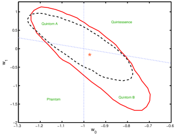
Figure 1: Two dimensional constraints on $(w_{0},w_{1})$ from current observations of CMB $+$ SNIa $+$ BAO. The red solid and black dash lines represent the 2 $\sigma$ limits for the two cases with and without dark energy perturbations, respectively. The star represents the best fit value.

IV Summary and Discussion

In this paper we have revisited the dynamics of cosmological perturbations of dark energy and paid particular attention to the case when the EoS crosses the cosmological constant boundary. Single field or single fluid models, or scenarios based on a parameterized EoS of dark energy with a single component cannot cross $w_{D}=-1$ because the perturbations are singular and unstable at this point. The quintom model is able to cross this boundary naturally, however it requires more degrees of freedom, and lessons learned when studying the transfer of fluctuations through non-singular bounces makes us expect that, on scales smaller than the time duration of the transition phase, the final fluctuations will depend on the details of the model. This makes it hard to obtain a simple data fitting prescription. In particular, the more parameters are introduced, the more computing time is required for the numerical calculations. To obtain a simple way of analyzing data and assessing the observational evidence for or against the equation of state of dark energy crossing the cosmological constant divide it is thus very useful to have a prescription which does not introduce new parameters.

In this paper we have presented a new approach to studying dark energy perturbations in the time interval when [ $w_{+}=-1+\epsilon,~{}w_{-}=-1-\epsilon$ ] , i.e. during the crossing of the boundary $w_{D}=-1$. We have proposed to apply the general relativistic matching conditions of Hwang:1991an ; Deruelle:1995kd . These conditions imply that the dark energy perturbations match continuously on the two sides of the surface $w_{D}=-1$.

Let us mention some caveats to our analysis: Our method is applicable in the form presented here only if on either side of the matching surface all except for one fluid are negligible. Since at the crossing region this assumption will fail, this criterium implies that $\epsilon$ cannot be too small. Secondly, since the dark energy fluctuations diverge when the equation of state crosses the cosmological constant line, then, in order to stay within the realm of applicability of linear cosmological perturbation theory, we have a second reason why $\epsilon$ cannot be taken to be too small. On the other hand, for length scales smaller than $\epsilon t$, where $t$ is the time when the EoS of dark energy crosses the cosmological constant line, the way in which the fluctuations pass through the transition region may depend on the specific quintom models. This argument prefers a small value for $\epsilon$.

However, let us consider models where our assumptions are satisfied and where $\epsilon$ is sufficiently small. Then, our results coincide with those of Ref. Zhao:2005vj , and the arguments in this paper justify the method used in the numerical calculations of xia1 ; xia2 ; xia3 . Since linear perturbation theory will break down as $\epsilon\rightarrow 0$, the small positive parameter $\epsilon$ would not be taken to be too small. In Ref. Zhao:2005vj it has been checked that with $\epsilon\sim 10^{-5}$, linear perturbation theory will be valid and at the same time the approximation of taking $\delta_{D}$ and $\theta_{D}$ to be constant in the interval [$w_{+}=-1+\epsilon,~{}w_{-}=-1-\epsilon$ ] will yield results in agreement with those obtained by using actual quintom perturbations.

Finally, with the method outlined in this paper we have performed a numerical determination of cosmological parameters. Our numerical results show explicitly the significance of the dark energy perturbations.

V acknowledgments

We thank Jun-Qing Xia and Gong-Bo Zhao for helpful comments and discussions. M.L. is supported by the Specialized Research Fund for the Doctoral Program of Higher Education (SRFDP) under Grant No. 20090091120054. Y.C., H.L. and X.Z. are supported in part by the National Natural Science Foundation of China under Grants Nos. 10975142, 10821063 and 10803001 and by the 973 program Nos. 1J2007CB81540002 and 2010CB833000 and by the Youth Foundation of the Institute of High Energy Physics under Grant No. H95461N. R.B. is supported in part by funds from NSERC and from the CRC program of Canada. He also wishes to acknowledge the warm hospitality of the cosmology group at the Institute of High Energy Physics during a visit when this project was started.

References

- (1) G. B. Zhao, J. Q. Xia, M. Li, B. Feng and Xinmin Zhang, “Perturbations of the Quintom Models of Dark Energy and the Effects on Observations,” Phys. Rev. D 72, 123515 (2005) [arXiv:astro-ph/0507482].
- (2) J. Q. Xia, G. B. Zhao, B. Feng, H. Li and Xinmin Zhang, “Observing Dark Energy Dynamics with Supernova, Microwave Background and Galaxy Clustering,” Phys. Rev. D 73, 063521 (2006) [arXiv:astro-ph/0511625].
- (3) G. B. Zhao, J. Q. Xia, B. Feng and Xinmin Zhang, “Probing dynamics of dark energy with supernova, galaxy clustering and the three-year Wilkinson Microwave Anisotropy Probe (WMAP) observations,” Int. J. Mod. Phys. D 16 (2007) 1229 [arXiv:astro-ph/0603621].
- (4) J. Q. Xia, H. Li, G. B. Zhao and Xinmin Zhang, “Determining Cosmological Parameters with Latest Observational Data,” Phys. Rev. D 78 (2008) 083524 [arXiv:0807.3878 [astro-ph]].
- (5) A. G. Riess et al. [Supernova Search Team Collaboration], “Observational Evidence from Supernovae for an Accelerating Universe and a Cosmological Constant,” Astron. J. 116, 1009 (1998) [arXiv:astro-ph/9805201].
- (6) S. Perlmutter et al. [Supernova Cosmology Project Collaboration], “Measurements of Omega and Lambda from 42 High-Redshift Supernovae,” Astrophys. J. 517, 565 (1999) [arXiv:astro-ph/9812133].
- (7) B. Ratra and P. J. E. Peebles, “Cosmological Consequences of a Rolling Homogeneous Scalar Field,” Phys. Rev. D 37, 3406 (1988).
- (8) C. Wetterich, “Cosmology and the Fate of Dilatation Symmetry,” Nucl. Phys. B 302, 668 (1988).
- (9) R. R. Caldwell, R. Dave and P. J. Steinhardt, “Cosmological Imprint of an Energy Component with General Equation-of-State,” Phys. Rev. Lett. 80, 1582 (1998) [arXiv:astro-ph/9708069].
- (10) R. R. Caldwell, “A Phantom Menace?,” Phys. Lett. B 545, 23 (2002) [arXiv:astro-ph/9908168].
- (11) C. Armendariz-Picon, V. F. Mukhanov and P. J. Steinhardt, “A dynamical solution to the problem of a small cosmological constant and late-time cosmic acceleration,” Phys. Rev. Lett. 85, 4438 (2000) [arXiv:astro-ph/0004134].
- (12) B. Feng, X. Wang and Xinmin Zhang, “Dark Energy Constraints from the Cosmic Age and Supernova,” Phys. Lett. B 607, 35 (2005) [arXiv:astro-ph/0404224].
- (13) E. J. Copeland, M. Sami and S. Tsujikawa, “Dynamics of dark energy,” Int. J. Mod. Phys. D 15, 1753 (2006) [arXiv:hep-th/0603057].
- (14) A. J. Albrecht et al., “Report of the Dark Energy Task Force,” arXiv:astro-ph/0609591.
- (15) E. V. Linder, “Mapping the Cosmological Expansion,” Rept. Prog. Phys. 71, 056901 (2008) [arXiv:0801.2968 [astro-ph]].
- (16) R. R. Caldwell and M. Kamionkowski, “The Physics of Cosmic Acceleration,” Ann. Rev. Nucl. Part. Sci. 59, 397 (2009) [arXiv:0903.0866 [astro-ph.CO]].
- (17) A. Silvestri and M. Trodden, “Approaches to Understanding Cosmic Acceleration,” Rept. Prog. Phys. 72, 096901 (2009) [arXiv:0904.0024 [astro-ph.CO]].
- (18) Y. F. Cai, E. N. Saridakis, M. R. Setare and J. Q. Xia, “Quintom Cosmology: Theoretical implications and observations,” arXiv:0909.2776 [hep-th].
- (19) S. Nesseris and L. Perivolaropoulos, “Crossing the Phantom Divide: Theoretical Implications and Observational Status,” JCAP 0701, 018 (2007) [arXiv:astro-ph/0610092].
- (20) M. Chevallier and D. Polarski, “Accelerating universes with scaling dark matter,” Int. J. Mod. Phys. D 10, 213 (2001) [arXiv:gr-qc/0009008].
- (21) E. V. Linder, “Exploring the expansion history of the universe,” Phys. Rev. Lett. 90, 091301 (2003) [arXiv:astro-ph/0208512].
- (22) J. Q. Xia, Y. F. Cai, T. T. Qiu, G. B. Zhao and Xinmin Zhang, “Constraints on the Sound Speed of Dynamical Dark Energy,” Int. J. Mod. Phys. D 17, 1229 (2008) [arXiv:astro-ph/0703202].
- (23) R. Bean and O. Dore, “Probing dark energy perturbations: the dark energy equation of state and speed of sound as measured by WMAP,” Phys. Rev. D 69, 083503 (2004) [arXiv:astro-ph/0307100].
- (24) J. Q. Xia, G. B. Zhao, B. Feng, H. Li and Xinmin Zhang, “Observing Dark Energy Dynamics with Supernova, Microwave Background and Galaxy Clustering,” Phys. Rev. D 73, 063521 (2006) [arXiv:astro-ph/0511625].
- (25) E. Komatsu et al. [WMAP Collaboration], “Five-Year Wilkinson Microwave Anisotropy Probe (WMAP ) Observations:Cosmological Interpretation,” Astrophys. J. Suppl. 180, 330 (2009) [arXiv:0803.0547 [astro-ph]].
- (26) C. Yeche, A. Ealet, A. Refregier, C. Tao, A. Tilquin, J. M. Virey and D. Yvon, “Prospects for Dark Energy Evolution: a Frequentist Multi-Probe Approach,” arXiv:astro-ph/0507170.
- (27) A. Vikman, “Can dark energy evolve to the phantom?,” Phys. Rev. D 71, 023515 (2005) [arXiv:astro-ph/0407107].
- (28) W. Hu, “Crossing the phantom divide: Dark energy internal degrees of freedom,” Phys. Rev. D 71, 047301 (2005) [arXiv:astro-ph/0410680].
- (29) R. R. Caldwell and M. Doran, “Dark-energy evolution across the cosmological-constant boundary,” Phys. Rev. D 72, 043527 (2005) [arXiv:astro-ph/0501104].
- (30) M. Li, B. Feng and Xinmin Zhang, “A single scalar field model of dark energy with equation of state crossing -1,” JCAP 0512, 002 (2005) [arXiv:hep-ph/0503268].
- (31) X. F. Zhang, H. Li, Y. S. Piao and Xinmin Zhang, “Two-field models of dark energy with equation of state across -1,” Mod. Phys. Lett. A 21, 231 (2006) [arXiv:astro-ph/0501652].
- (32) M. Kunz and D. Sapone, “Crossing the Phantom Divide,” Phys. Rev. D 74, 123503 (2006) [arXiv:astro-ph/0609040].
- (33) W. Fang, W. Hu and A. Lewis, “Crossing the Phantom Divide with Parameterized Post-Friedmann Dark Energy,” Phys. Rev. D 78, 087303 (2008) [arXiv:0808.3125 [astro-ph]].
- (34) W. Hu, “Parametrized Post-Friedmann Signatures of Acceleration in the CMB,” Phys. Rev. D 77, 103524 (2008) [arXiv:0801.2433 [astro-ph]].
- (35) W. Hu and I. Sawicki, “A Parameterized Post-Friedmann Framework for Modified Gravity,” Phys. Rev. D 76, 104043 (2007) [arXiv:0708.1190 [astro-ph]].
- (36) J. c. Hwang and E. T. Vishniac, “Gauge-invariant joining conditions for cosmological perturbations,” Astrophys. J. 382, 363 (1991).
- (37) N. Deruelle and V. F. Mukhanov, “On matching conditions for cosmological perturbations,” Phys. Rev. D 52, 5549 (1995) [arXiv:gr-qc/9503050].
- (38) W. Israel, “Singular hypersurfaces and thin shells in general relativity,” Nuovo Cim. B 44S10, 1 (1966) [Erratum-ibid. B 48, 463 (1967)] [Nuovo Cim. B 44, 1 (1966)].
- (39) R. Durrer and F. Vernizzi, “Adiabatic perturbations in pre big bang models: Matching conditions and scale invariance,” Phys. Rev. D 66, 083503 (2002) [arXiv:hep-ph/0203275].
- (40) R. Brandenberger and F. Finelli, “On the spectrum of fluctuations in an effective field theory of the ekpyrotic universe,” JHEP 0111, 056 (2001) [arXiv:hep-th/0109004].
- (41) J. c. Hwang, “Cosmological structure problem in the ekpyrotic scenario,” Phys. Rev. D 65, 063514 (2002) [arXiv:astro-ph/0109045].
- (42) F. Finelli and R. Brandenberger, “On the generation of a scale-invariant spectrum of adiabatic fluctuations in cosmological models with a contracting phase,” Phys. Rev. D 65, 103522 (2002) [arXiv:hep-th/0112249].
- (43) Y. F. Cai, T. T. Qiu, R. Brandenberger, Y. S. Piao and Xinmin Zhang, “On Perturbations of Quintom Bounce,” JCAP 0803, 013 (2008) [arXiv:0711.2187 [hep-th]].
- (44) Y. F. Cai and Xinmin Zhang, “Evolution of Metric Perturbations in Quintom Bounce model,” JCAP 0906, 003 (2009) [arXiv:0808.2551 [astro-ph]].
- (45) Y. F. Cai, T. T. Qiu, R. Brandenberger and Xinmin Zhang, “A Nonsingular Cosmology with a Scale-Invariant Spectrum of Cosmological Perturbations from Lee-Wick Theory,” Phys. Rev. D 80, 023511 (2009) [arXiv:0810.4677 [hep-th]];
- (46) V. F. Mukhanov, H. A. Feldman and R. H. Brandenberger, “Theory of cosmological perturbations. Part 1. Classical perturbations. Part 2. Quantum theory of perturbations. Part 3. Extensions,” Phys. Rept. 215, 203 (1992).
- (47) C. P. Ma and E. Bertschinger, “Cosmological perturbation theory in the synchronous and conformal Newtonian gauges,” Astrophys. J. 455, 7 (1995) [arXiv:astro-ph/9506072].
- (48) Y. F. Cai, T. Qiu, Y. S. Piao, M. Li and Xinmin Zhang, “Bouncing Universe with Quintom Matter,” JHEP 0710, 071 (2007) [arXiv:0704.1090 [gr-qc]].
- (49) Y. F. Cai, T. T. Qiu, J. Q. Xia and Xinmin Zhang, “A Model Of Inflationary Cosmology Without Singularity,” Phys. Rev. D 79, 021303 (2009) [arXiv:0808.0819 [astro-ph]]; Y. F. Cai and Xinmin Zhang, “Primordial perturbation with a modified dispersion relation,” Phys. Rev. D 80, 043520 (2009) [arXiv:0906.3341 [astro-ph.CO]].
- (50) E. Komatsu et al., “Seven-Year Wilkinson Microwave Anisotropy Probe (WMAP) Observations: Cosmological Interpretation,” arXiv:1001.4538 [astro-ph.CO].
- (51) C. J. MacTavish, et al., Astrophys. J. 647, 799 (2006).
- (52) A. C. S. Readhead, et al., Astrophys. J. 609, 498 (2004).
- (53) C. Dickinson, et al., Mon. Not. Roy. Astron. Soc. 353, 732 (2004).
- (54) C. L. Reichardt, et al., arXiv:0801.1491.
- (55) R. Amanullah et al., “Spectra and Light Curves of Six Type Ia Supernovae at 0.511 ¡ z ¡ 1.12 and the Union2 Compilation,” Astrophys. J. 716, 712 (2010) [arXiv:1004.1711 [astro-ph.CO]].
- (56) W. J. Percival et al., “Baryon Acoustic Oscillations in the Sloan Digital Sky Survey Data Release 7 Galaxy Sample,” Mon. Not. Roy. Astron. Soc. 401, 2148 (2010) [arXiv:0907.1660 [astro-ph.CO]].
- (57) H. Li, J. Q. Xia, G. B. Zhao, Z. H. Fan and Xinmin Zhang, “On using the WMAP distance priors in constraining the time evolving equation of state of dark energy,” Astrophys. J. 683, L1 (2008) [arXiv:0805.1118 [astro-ph]].