Proton scattering observables from Skyrme-Hartree-Fock densities

Abstract

Proton and neutron densities from Skyrme-Hartree-Fock (SHF) calculations are used to generate non-local ($g$-folding) proton-nucleus optical potentials. They are formed by folding the densities with realistic nucleon-nucleon interactions. The potentials are then used to calculate differential cross sections and spin observables for proton scattering. Good agreement with data has been found, supporting those found previously when using SHF charge densities in analyses of electron scattering data. That agreement was improved by use of (shell model) occupation numbers to constrain the HF iterations. That, in part, is also the case with analyses of proton scattering data. The $g$-folding method is extended to exotic nuclei by including data for neutron-rich $sd$-shell nuclei from the inverse kinematics of scattering from hydrogen.

I Introduction

Nucleon-nucleus ($NA$) scattering probes the matter density of the nucleus, and of particular interest are the separate density distributions of protons and neutrons. The differences between the two densities become increasingly important as one moves away from the valley of stability towards the drip lines, with the emergence of structures such as halos and skins. Those structures influence $NA$ scattering, whence the problem becomes one of how to extract such information from measurement. For detailed information on the matter (proton and/or neutron) density of the target nucleus one requires a microscopic description of the interaction between the projectile and the target, necessitating also a microscopic (nucleon-based) description of the nucleus.

For radioactive nuclei, experiments have been done in inverse kinematics with a beam of nuclei incident on a hydrogen target. Thus the calculation of differential cross sections and spin observables requires some microscopic model structure for the exotic nucleus, which determines the ground-state densities. The adequacy of the model assumed, for stable nuclei, can be checked against information obtained from the elastic scattering of electrons. The electron scattering form factors are measures of the charge and current densities of the nucleus. While electron scattering data for exotic nuclei are not presently available, the SCRIT experiment Su05 ; *Su09 and the electron-ion collider ELISe at FAIR Si05 will measure such form factors. At present, one must rely on model predictions for the matter densities and test those against proton scattering data.

Proton and neutron ground-state densities have been determined for a wide range of nuclei from Skyrme-Hartree-Fock (SHF) calculations, and extensive comparisons for the charge densities have been made with available data from electron scattering Ri03 . The good agreement generally found reflects on the adequacy of the calculated matter densities, which are used as input for the calculation of proton elastic scattering observables in this work. Analyses of proton scattering data from ²⁰⁸Pb using SHF models have been made Ka02 , whereby the neutron skin thickness in ²⁰⁸Pb was determined. One corollary of the latter was the observation that analyses of zero momentum transfer data are not enough to elicit sufficient information on the densities of nuclei. Data taken at finite momentum transfer are also required. For analyses of proton scattering data to have credibility, as tests of the underlying structures assumed for the target nuclei, one must have a model of scattering for which there are no parameters to be fitted to the data being analysed. Only then may one evaluate the models used to specify the nuclear structure without ambiguity.

The matter densities obtained from the assumed structure models (shell, SHF, and SHF with shell-model occupancies) have been used with realistic nucleon-nucleon interactions in a folding model, requiring no a posteriori fitting Am00 , to specify optical potentials for the elastic scattering of protons with energies in the range $25-200$ MeV. Those potentials are then used to make predictions for differential cross sections and spin observables for proton scattering, a procedure that has been applied extensively Am00 . Comparisons are then made to available proton scattering data. When using that folding model with the SHF densities, those allowed for the recognition of a signature for exotic structures in neutron-rich isotopes in the reaction cross sections Am06 . The present work extends that earlier work to consider the effects on the elastic scattering observables.

II The Skyrme-Hartree-Fock density calculations

Charge-density distributions and the associated nuclear radii have been calculated with the Hartree-Fock method for comparison with available data from electron scattering Ri03 . Two forms of the Skyrme interaction have been used for the calculations, the so-called SKX${}_{\text{csb}}$ Br00 and SKM* Ba82 interactions. The SKX${}_{\text{csb}}$ Hamiltonian is based on the SKX Hamiltonian Br98 with a charge-symmetry-breaking (CSB) interaction, added to account for nuclear displacement energies Br00 . The charge densities from SKX and SKX${}_{\text{csb}}$ are essentially identical, so the SKX${}_{\text{csb}}$ results will be referred to as ”SKX”. The SKX and SKM* results for the charge densities are very similar, the main difference being that the interior density is about 5% higher with SKM*, with marginally better overall agreement with experiment for SKM*. Generally good agreement between theory and experiment has been achieved in extensive comparisons of measured nuclear charge-density distributions with calculated values for $p$-shell, $sd$-shell, and $fp$-shell nuclei and some selected magic and semi-magic nuclei up to Pb. The extent of the agreement is further improved by constraining the Hartree-Fock equations to use occupation numbers from large-basis shell model calculations. Somewhat larger deviations are observed for lighter nuclei, which may imply the inadequacy of the mean-field approximation Ri03 . The good agreement with experiment for electron scattering data is a justification for using the proton and neutron radial wave functions as input for the optical model calculations.

For the purposes of the present study, we have used both the basic SHF (denoted SHF henceforth) densities and those obtained from the SHF constrained by use of the shell model occupation numbers (denoted as SHF-SM). (Those numbers are listed in Table 1 for the isotopes considered herein.)

Table 1: Shell-model occupation numbers, as used in the SHF-SM calculations, for the given orbits.
(Nomenclature: $4=0d_{5/2},5=0d_{3/2},6=1s_{1/2},7=0f_{7/2},8=0f_{5/2},9=1p_{3/2},10=1p_{1/2}$)

Z	Isotope	Orbits	Proton occupancies	Neutron occupancies
14	28Si	4, 5, 6	$4.623,0.673,0.704$	$4.623,0.673,0.704$
16	32S	4, 5, 6	$5.421,1.161,1.418$	$5.421,1.161,1.418$
16	34S	4, 5, 6	$5.607,0.736,1.657$	$5.674,2.484,1.752$
16	36S	4, 5, 6	$5.869,0.237,1.894$	$6.000,4.000,2.000$
16	38S	4, 5, 6	$5.766,0.762,1.472$
		7, 8, 9, 10		$1.636,0.088,0.242,0.034$
16	40S	4, 5, 6	$5.727,1.302,0.972$
		7, 8, 9, 10		$3.350,0.156,0.443,0.052$
18	36Ar	4, 5, 6	$5.761,2.500,1.740$	$5.761,2.500,1.740$
18	38Ar	4, 5, 6	$5.946,2.109,1.945$	$6.000,4.000,2.000$
18	40Ar	4, 5, 6	$5.920,2.200,1.880$
		7, 8, 9, 10		$1.750,0.060,0.160,0.030$
18	44Ar	4, 5, 6	$5.840,2.659,1.491$
		7, 8, 9, 10		$5.359,0.193,0.397,0.051$
20	40Ca	5, 6, 7, 9	$3.090,1.800,0.990,0.120$	$3.090,1.800,0.990,0.120$
20	42Ca	7, 8, 9, 10		$1.812,0.058,0.110,0.021$
20	44Ca	7, 8, 9, 10		$3.674,0.126,0.171,0.029$
20	48Ca	5, 6, 7, 9	$3.550,1.630,0.750,0.070$	$3.830,1.960,7.910,0.300$

For the $sd$-shell, the USD interaction of Wildenthal and Brown Br88 as well as the USDB interaction of Brown and Richter Br06 , in the case of the neutron-rich nuclei, were used. For those nuclei in which the neutrons extend to the $fp$-shell the sdpf-U interaction of Nowacki and Poves No09 was used in the $sdpf$-model space. No spuriosity is admitted into the wave functions as the protons are restricted to be solely within the $sd$-shell. All calculations of the occupation numbers were done using the NuShell shell-model code Nu10 . For comparison, we have also used shell model wave functions where indicated for the lighter isotopes, and used a simple packed shell model in which the lowest orbits are filled, with no configuration mixing.

III Calculation of proton scattering observables

To calculate microscopically the differential cross sections and spin observables for $NA$ scattering, one generally begins with an effective nucleon-nucleon ($NN$) interaction. That interaction is folded with the ground-state density of the target nucleus to obtain the microscopic optical potential from which the observables are obtained. Herein, we utilise the Melbourne approach, which is described in detail in a review Am00 ; we give a brief outline to highlight the important aspects of this model below.

To obtain a credible effective $NN$ interaction one usually starts with the $g$ matrices of the free $NN$ interaction. Those $g$ matrices are solutions of the Brueckner-Bethe-Goldstone (BBG) equations for infinite nuclear matter, viz.

$$g\left(\mathbf{q}^{\prime},\mathbf{q};\mathbf{K}\right)=V\left(\mathbf{q}^{\prime},\mathbf{q}\right)+\int V\left(\mathbf{q}^{\prime},\mathbf{k}^{\prime}\right)\frac{Q\left(\mathbf{k}^{\prime},\mathbf{K};k_{f}\right)}{\left[E\left(\mathbf{k},\mathbf{K}\right)-E\left(\mathbf{k}^{\prime},\mathbf{K}\right)\right]}\,g\left(\mathbf{k}^{\prime},\mathbf{q};\mathbf{K}\right)\,d\mathbf{k}^{\prime},$$ (1)

where $Q$ is a Pauli blocking operator, and effects of the mean field are incorporated into the auxiliary potentials entering the energy denominator. The centre-of-mass and Fermi momenta are denoted by $K$ and $k_{f}$, respectively.

The $g$ matrices obtained from the BBG equations are mapped to a coordinate-space representation to give an effective $g$ matrix ($g_{\text{eff}}$) which is complex, energy- and density-dependent. When that effective interaction is folded with a reasonable microscopic model structure of the target for the nucleus, one obtains the $NA$ optical potential of the form,

$$U\left(\mathbf{r},\mathbf{r}^{\prime};E\right) =\delta\left(\mathbf{r}-\mathbf{r}^{\prime}\right)\sum_{i}n_{i}\int\varphi^{\ast}_{i}(\mathbf{s})g_{D}\left(\mathbf{r},\mathbf{s};E\right)\varphi_{i}(\mathbf{s})\,d\mathbf{s}+\sum_{i}n_{i}\varphi^{\ast}_{i}(\mathbf{r})g_{E}\left(\mathbf{r},\mathbf{r}^{\prime};E\right)\varphi_{i}(\mathbf{r}^{\prime})$$

$$=U_{D}\left(\mathbf{r};E\right)\delta\left(\mathbf{r}-\mathbf{r}^{\prime}\right)+U_{E}\left(\mathbf{r},\mathbf{r}^{\prime};E\right),$$ (2)

where the subscripts $D,E$ denote the (local) direct and (nonlocal) exchange parts of the optical potential, respectively. The sums are taken over the bound state single-particle orbits for which $n_{i}$ are the associated occupation numbers. We use a variant of the DWBA98 program Ra98 to calculate the optical potential and observables using SHF single-particle wave functions. The resultant complex, energy-, and density-dependent $g$-folding optical potential contains central, two-body spin-orbit, and tensor terms. As there are no parameter adjustments to fit to the data being described, all model results are predictions.

IV Comparisons with data

We present analyses with reference to various isotopes of S, Ar, and Ca, as listed in Table 2, together with references to available data as used in these analyses.

Table 2: Isotopes considered for the elastic scattering of protons. References for the available data are given.

Nuclei	References
28Si	Ka85 , Hi88 ; *Lu92
32S, 34S, 36S, 38S, 40S	Ka85 , Le80 , Al85 , Ho90 , Ke97 , Ma99
36Ar, 38Ar, 40Ar, 42Ar, 44Ar	Sc00 , Sa82
40Ca, 42Ca, 44Ca, 46Ca, 48Ca, 50Ca, 52Ca, 54Ca	Sa82 , No81

In the following diagrams, except when explicitly specified, the results of the calculations made using the shell (or packed shell), SHF, and SHF-SM models are denoted by the solid, dashed, and dot-dashed lines, respectively.

Before considering the S, Ar, and Ca isotopes, we consider scattering from ²⁸Si, as there are many data available for this stable nucleus. Of the elastic proton scattering data available, we have chosen to analyse those data taken at 65 MeV Ka85 and 200 MeV Hi88 , as there have been extensive analyses of data for a range of nuclei at both energies Do97 ; *Do98, resulting in the effective $NA$ interactions at both energies being well-established. Fig. 1 presents the differential cross sections and analysing powers for the elastic scattering

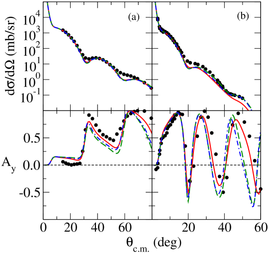
Figure 1: (Color online.) Differential cross sections and analysing powers for the elastic scattering of 65 [(a)] and 200 MeV [(b)] protons from ²⁸Si. The data are compared to the results of calculations made using the shell, SHF, and SHF-SM models.

of protons from ²⁸Si, wherein the data are compared to the results of the calculations made using wave functions from the shell, SHF, and the SHF-SM models. The oscillator length for the harmonic oscillator single-particle wave functions used in the shell model calculation was 1.85 fm. For 65 MeV scattering there is very little difference in the predictions for the differential cross sections between the three models used; they do equally well in describing the data. Differences emerge in the analysing power, with the shell model result doing best of all, although all three results describe the shape and magnitudes well. While the three models do well to describe the forward-angle differential cross section at 200 MeV, both SHF models do better in predicting the cross section above $20^{\circ}$. In the results for the analysing power at that energy, the shell-model result deviates significantly from the SHF results above $20^{\circ}$ but are in better agreement with the data.

IV.1 The S isotopes

Fig. 2 displays the results of calculations made for the elastic scattering of 65 MeV protons from ³²S.

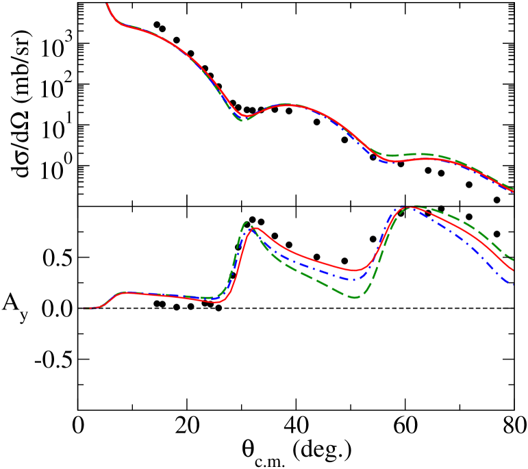
Figure 2: (Color online.) Differential cross sections and analysing powers for the elastic scattering of 65 MeV protons from ³²S. The data are compared to the results of calculations made using the shell, SHF, and SHF-SM models.

Therein, the data Ka85 are compared to the results obtained from the shell ($b=1.85$ fm), SHF, and SHF-SM models. All three models give a reasonable representation of the differential cross-section data to $60^{\circ}$, but overestimate the differential cross section at larger angles. The differences between the models are far more noticeable in the analysing power, for which the shell model result gives clearly the best agreement with data. Of the two SHF models, the model with the shell model occupancies defined a priori gives the better agreement. This is of note as ³²S is mid-shell and the occupancies are expected to play a significant role. We have also considered the elastic scattering of 29.6 MeV protons from ³²S, the results of which are shown in Fig. 3.

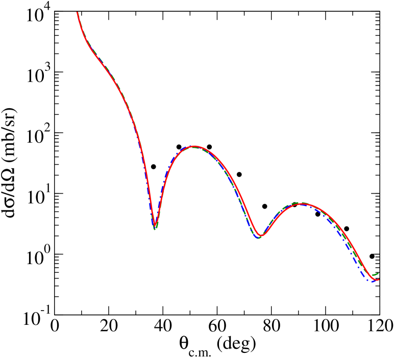
Figure 3: (Color online.) As for Fig. 2 but for 29.6 MeV protons.

There is agreement between all the models and reasonable agreement with the data Le80 . It is worth noting that the present analysis reproduces the shape and magnitude well, without the need for ad hoc renormalisations of potentials or the use of the phenomenological $M_{n}/M_{p}$ ratios Ma99 , which has been shown to be problematic Am10 .

The results of the calculations from the three models for the scattering of 29.8 MeV protons from ³⁴S are compared to the data Al85 in Fig. 4.

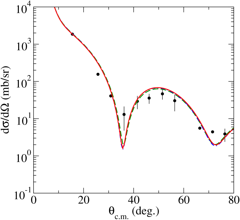
Figure 4: (Color online.) As for Fig. 2 but for the elastic scattering of 29.8 MeV protons from ³⁴S.

For ³⁴S, there is very little difference between the results obtained using the shell model (the same oscillator length was used as for ³²S) or either of the SHF models. All results are in quite reasonable agreement with the available data Al85 . This is consistent with the results for the scattering at 29.6 MeV for ³²S.

Fig. 5 shows the differential cross section for the elastic scattering of 28 MeV protons from ³⁶S.

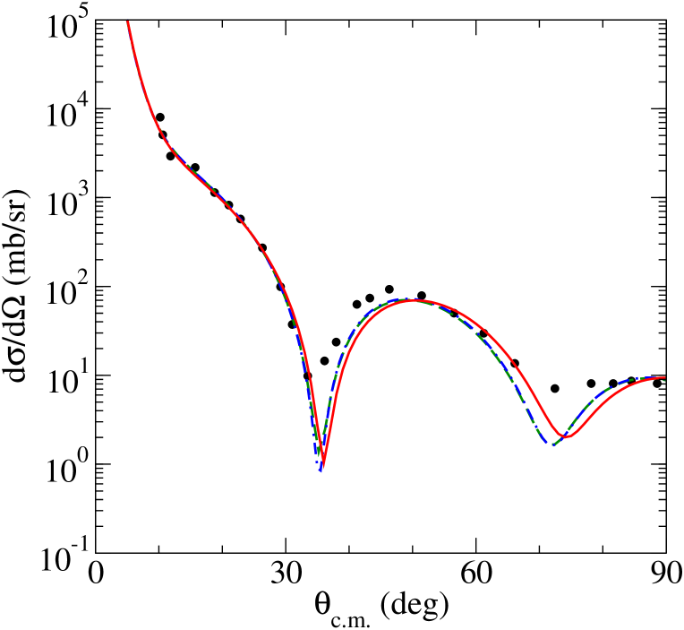
Figure 5: (Color online.) As for Fig. 2, but for the elastic scattering of 28 MeV protons from ³⁶S.

Therein, the results of the calculations made using the shell ($b=1.9$ fm), SHF, and SHF-SM models are compared to the data Ho90 . All models do equally well in describing the data, although the level of agreement between the results and the data above $35^{\circ}$ is somewhat poorer. Considering the problems in specifying the microscopic optical potentials below 30 MeV Am00 , the level of agreement is still reasonable. A previous JLM analysis Ma99 was able to reproduce the data, but only by renormalising the real and imaginary parts of the potential. Also, in that case, the isovector part of the JLM potential was increased by a factor of 2.0. No such renormalisations were required in the potential for the results in the present work.

The differential cross section for the elastic scattering of 39 MeV protons from ³⁸S is shown in Fig. 6.

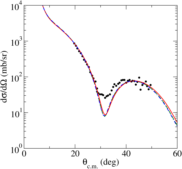
Figure 6: (Color online.) As for Fig. 2, but for the elastic scattering of 39 MeV protons from ³⁸S. The shell model used in this case is a packed model.

Therein, the three models ($b=1.9$ fm for the packed shell model) are compared to the data Ke97 . All the models do equally well in describing the data up to $30^{\circ}$. All the models underestimate the data in the region of the minimum, up to $40^{\circ}$. The previous JLM model result Ma99 required a larger renormalisation of the imaginary part of the potential compared to the real part, which was not in keeping with the normalisations that model required for the lighter isotopes.

Fig. 7 shows the differential cross section for 30 MeV elastic scattering of protons from ⁴⁰S.

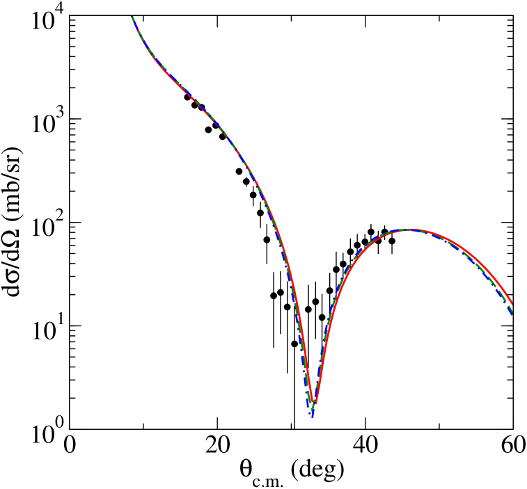
Figure 7: (Color online.) As for Fig. 6, but for the elastic scattering of 30 MeV protons from ⁴⁰S.

Therein, the data Ma99 are compared to the results from the packed shell ($b=1.9$ fm), SHF, and SHF-SM models. All the results compare equally well with the data, and once more no renormalisations in the potentials were necessary in achieving these results. However, the level of agreement is difficult to gauge given the large error bars in the data.

IV.2 The Ar isotopes

We now turn our attention to the Ar isotopes, beginning with ³⁶Ar. Fig. 8 shows the comparison

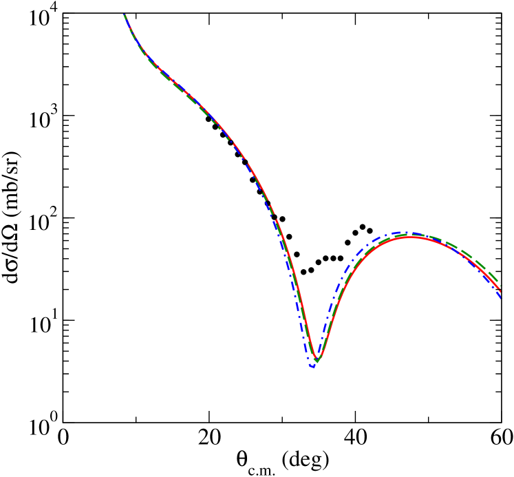
Figure 8: (Color online.) Differential cross section for the elastic scattering of 33 MeV protons from ³⁶Ar. The data Sc00 are compared to the results of the calculations made using wave functions obtained from the shell, the SHF, and the SHF-SM models.

of the data to the results of the calculations made using the wave functions from the shell ($b=1.85$ fm), basic SHF, and SHF-SM models. All model results agree with the data up to $32^{\circ}$ quite well. However, beyond that the model results do not reproduce either the shape or the magnitude of the data, although the SHF-SM result does marginally better than the other two. An earlier microscopic (JLM model) analysis Sc00 required independent renormalisations of the real and imaginary parts of the effective $NA$ interaction of 0.94 and 0.92, respectively, to fit the data. One cannot conclude as to whether the reproduction of the data is due to the underlying description of the nucleus, or the renormalisations of the potential. Also, those data beyond $30^{\circ}$ do not define a sharp diffraction minimum, even one that may be smoothed by experimental resolution. Another measurement may be required to explain the anomalies between the models’ predictions and to confirm the data.

Fig. 9 presents the results of calculations made for the elastic scattering of 33 and 65 MeV protons from ³⁸Ar using wave functions from the three models, where $b=1.85$ fm is used for the shell model densities.

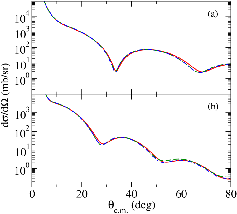
Figure 9: (Color online.) Comparison of the differential cross sections obtained from calculations made using the shell, SHF, and SHF-SM models for the elastic scattering of 33 MeV (a) and 65 MeV (b) protons from ³⁸Ar.

There is very little difference between the three models.

The differential cross sections and analysing powers for the elastic scattering of 65 MeV protons from ⁴⁰Ar are displayed in Fig. 10.

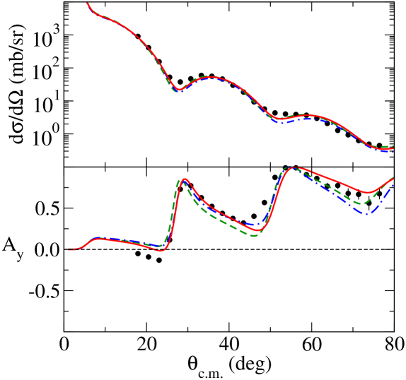
Figure 10: (Color online.) Differential cross section and analysing power for the elastic scattering of 65 MeV protons from ⁴⁰Ar. The data Sa82 are compared to the calculations made using a packed shell, the SHF, and the SHF-SM models.

Therein, the differential cross-section and analysing power data Sa82 are compared to the results of the calculations made using a simple packed shell model ($b=1.85$ fm), the SHF, and SHF-SM models. Of the three results, the best agreement with the data comes from using the simple packed model. The differential cross section is well reproduced also by the SHF model, while the SHF-SM model does marginally less well. For the analysing power, all three models explain the data reasonably well, though the best agreement is obtained with the packed shell model.

Fig. 11 shows the differential cross sections for the 33 MeV elastic scattering of protons from ⁴²Ar and ⁴⁴Ar.

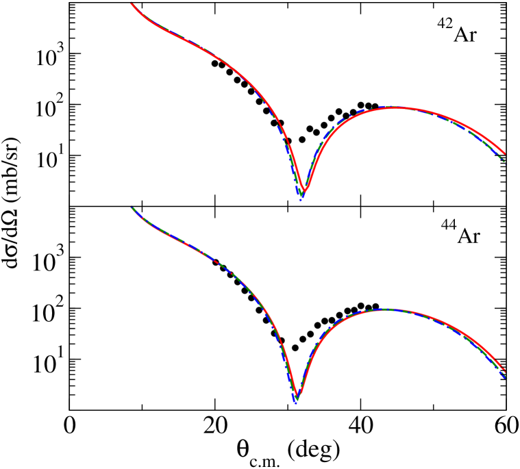
Figure 11: (Color online.) Differential cross sections for the scattering of 33 MeV protons from ⁴²Ar and ⁴⁴Ar. The data Sc00 are compared to the results of the calculations from the packed shell, SHF, and SHF-SM models.

Therein, the data Sc00 are compared to the results of the calculations made using the simple packed ($b=1.85$ fm and 1.88 fm for ⁴²Ar and ⁴⁴Ar, respectively), the SHF, and SHF-SM models. For both nuclei, there is no difference between the SHF and SHF-SM results. For ^36,42,44Ar, the models all give good results for scattering to $\sim 30^{\circ}$, and underestimate the cross section at larger angles. While the discrepancy is not as severe, and there is some agreement between the model results and the data at larger angles in magnitude and shape, we note that these data are from the same experiment as that for ³⁶Ar. The JLM analysis presented in the earlier work Sc00 required the same renormalisations of the real and imaginary parts. There is consistency in those JLM analyses but the question remains as to whether the level of agreement is due to the underlying structure or the renormalisations themselves.

IV.3 The Ca isotopes

The differential cross section and analysing power for the elastic scattering of 65 MeV protons from ⁴⁰Ca are displayed in Fig. 12.

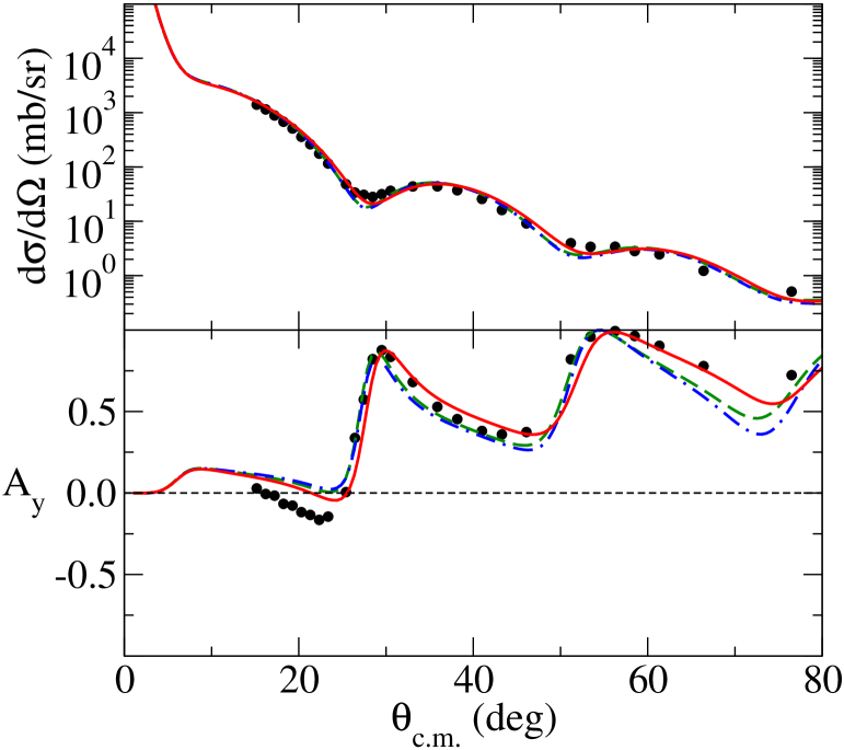
Figure 12: (Color online.) Differential cross section and analysing power for the elastic scattering of 65 MeV protons from ⁴⁰Ca. The data Sa82 are compared to the results of the calculations performed using a packed shell, SHF, and SHF-SM models.

Therein, the data Sa82 are compared to the results of calculations made using the packed shell ($b=1.9$ fm), the SHF, and SHF-SM models. All models do equally well in describing the differential cross-section data to $80^{\circ}$. It is in the analysing power that differences emerge, with the packed shell model providing a better description of the data.

Fig. 13 shows the differential cross section for the elastic scattering of 65 MeV protons from ⁴²Ca.

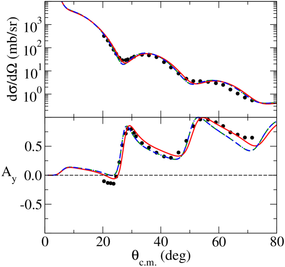
Figure 13: (Color online.) Differential cross section and analysing power for the elastic scattering of 65 MeV protons from ⁴²Ca. The data No81 are compared to the results of the packed shell model, SHF, and SHF-SM calculations.

The data No81 for the differential cross section are well described by the shell ($b=1.9$ fm) and both SHF models, as was the case for scattering from ⁴⁰Ca. As with ⁴⁰Ca, the packed shell model does better at describing the analysing power. Note that the results from the SHF models are identical, as the ground-state wave function is largely $(0f_{\frac{7}{2}})^{2}_{\nu}$, as indicated by the occupation numbers.

A similar observation may be reached for the comparison of the results of the calculations made from the packed shell ($b=1.9$ fm) and SHF models with data for the elastic scattering of 65 MeV protons from ⁴⁴Ca, for which the differential cross section and analysing power are displayed in Fig. 14.

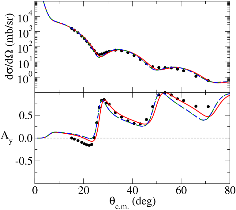
Figure 14: (Color online.) Differential cross section and analysing power for the elastic scattering of 65 MeV protons from ⁴⁴Ca. The data Sa82 are compared to the results of the calculations from the packed shell, SHF, and SHF-SM models.

Therein, the data Sa82 are compared to the results of the three model calculations. The results for the differential cross section compare quite well with the data, while the analysing power data are better described by the packed shell model result. As with ⁴²Ca, both SHF models give identical results, as the ground state is predominantly $(0f_{\frac{7}{2}})^{4}_{\nu}$.

⁴⁸Ca provides for an interesting test of the SHF models, as that nucleus is very well described by a filled $0f_{\frac{7}{2}}$ neutron shell. Fig. 15 displays the differential cross section and analysing power for

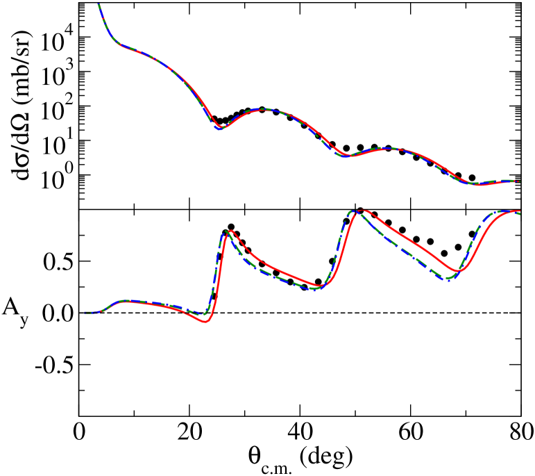
Figure 15: (Color online.) As for Fig. 12 but for the scattering from ⁴⁸Ca.

65 MeV elastic proton scattering from ⁴⁸Ca. The data Sa82 are compared to the results of the calculations made using all three models, where the shell model is a closed $0f_{\frac{7}{2}}$ neutron orbit ($b=1.9$ fm). All three results of the model calculations compare very well with the data. Yet, the SHF and SHF-SM models are almost in complete agreement: the SHF assumes a closed $0f_{\frac{7}{2}}$ neutron orbit, while the occupancies used in constraining the SHF-SM, listed in Table 1, indicate some mixing in ⁴⁸Ca. The degree of that mixing is small, and that is evident in the nearly identical predictions made between the SHF and SHF-SM models, for both the differential cross section and analysing power.

Fig. 16 displays the differential cross sections for the elastic scattering of 65 MeV protons from all even-even Ca isotopes from ⁴⁰Ca to ⁵⁴Ca. Therein, the SHF model was used to obtain the differential cross sections.

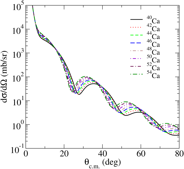
Figure 16: (Color online.) Differential cross sections for the elastic scattering of 65 MeV protons from all even-even Ca isotopes from ⁴⁰Ca to ⁵⁴Ca. The SHF model was used to obtain the cross sections.

As shown in the figure, there is a clear mass dependence in the differential cross section, as expected. Whether the cross sections for the heaviest Ca isotopes may be measured remains an academic question as it depends on the availability of suitable Ca beams. It is hoped that such beams will become available, as there is a question of the presence of a magic number either at ⁵²Ca or ⁵⁴Ca Ho02 . As the spin-orbit force may change close to the drip line, it has been suggested Ho02 that the $0f_{\frac{5}{2}}$ orbit falls below the $1p_{\frac{3}{2}}$, in which case ⁵²Ca would no longer be doubly-magic.

V Conclusions

We have presented results of calculations of elastic scattering of protons from isotopes of S, Ar, and Ca, using models based on Skyrme-Hartree-Fock methods. Two such models were used: one, the standard SHF, while the other constrained the Hartree-Fock iterations by specifying the nucleon occupancies, obtained from the shell model, a priori. For comparison, the shell model was also used to calculate the scattering observables.

Comparisons of results from calculations of proton elastic scattering from ²⁸Si indicated that using densities obtained from either the SHF models was as good, if not better, than using those from the shell model. Of the two SHF models, the SHF-SM model was found to be slightly better.

That the SHF-SM model gives a better description of the nuclear density was evident for ³²S since the differential cross section and analysing power were better described using that model structure. However, for the heavier isotopes of sulfur, that was not the case. Using either model for the structure, equivalent descriptions of the elastic scattering data were obtained. The shell model constraint on the Hartree-Fock procedure did not improve the level of agreement. It is of note that the descriptions of the elastic scattering worsened for large angles in these cases; serious renormalisations were required of the JLM potentials to obtain fits to the data. As the specification of the Melbourne potential does not allow for such renormalisations, we hope that more data may be collected to confirm the data used herein. The same conclusions were reached for the Ar isotopes, for which more data are also needed.

The Ca isotopes provided a sensitive control on the specification of the SHF densities, as ⁴⁸Ca is very well described by a filled $0f_{\frac{7}{2}}$ neutron shell. In that case, one expects the SHF and SHF-SM results to be equal. This was shown to be so in the analyses of the differential cross-section and analysing-power data for the elastic scattering. Also, we considered the mass dependence on the scattering from ⁴⁰Ca to ⁵⁴Ca and found that dependence to be smooth. As there is interest in the descriptions of the structures of ⁵²Ca and ⁵⁴Ca, we hope that scattering data will be measured in the future when beams of those two exotic nuclei become available.

Together with the reaction cross section, measurements of the differential cross sections will elicit much information on the structures of these neutron-rich nuclei. With the increase in the number of radioactive beam facilities it is hoped that not only will there be data taken for new nuclei, but also of those already available to provide valuable confirmation of previous experiments.

- (1) T. Suda and M. Wakasugi, Prog. Part. Nucl. Phys. 55, 417 (2005)
- (2) T. Suda et al., Phys. Rev. Lett. 102, 102501 (2009)
- (3) Technical Proposal for the Design, Construction, Commissioning, and Operation of the ELISe setup, spokesperson Haik Simon, GSI Internal Report, Dec. 2005
- (4) W. A. Richter and B. A. Brown, Phys. Rev. C 67, 034317 (2003)
- (5) S. Karataglidis, K. Amos, B. A. Brown, and P. K. Deb, Phys. Rev. C 65, 044306 (2002)
- (6) K. Amos, P. J. Dortmans, H. V. von Geramb, S. Karataglidis, and J. Raynal, Adv. in Nucl. Phys. 25, 275 (2000)
- (7) K. Amos, W. A. Richter, S. Karataglidis, and B. A. Brown, Phys. Rev. Lett. 96, 032503 (2006)
- (8) B. A. Brown, W. A. Richter, and R. Lindsay, Phys. Lett. B483, 49 (2000)
- (9) J. Bartel, P. Quentin, M. Brack, C. Guet, and M. B. Hakansson, Nucl. Phys. A386, 79 (1982)
- (10) B. A. Brown, Phys. Rev. C 58, 220 (1998)
- (11) B. A. Brown and B. H. Wildenthal, Ann. Rev. Nucl. Part. Sci. 36, 29 (1988)
- (12) B. A. Brown and W. A. Richter, Phys. Rev. C 74, 034315 (2006)
- (13) F. Nowacki and A. Poves, Phys. Rev. C 79, 014310 (2009)
- (14) NuShell Programme. http://www.nscl.msu.edu/brown/resources/resources.html
- (15) J. Raynal, “computer program dwba98, nea 1209/05,” (1998)
- (16) S. Kato et al., Phys. Rev. C 31, 1616 (1985)
- (17) K. H. Hicks et al., Phys. Rev. C 38, 229 (1988)
- (18) J. Lui et al., iUCF Scientific and Technical Report, 1992, p. 11
- (19) R. de Leo, G. D’Erasmo, E. M. Fiore, G. Guarino, and A. Pantaleo, Nuovo Cimento A 59, 101 (1980)
- (20) R. Alarcon, J. Rapaport, R. T. Kouzes, W. H. Moore, and B. A. Brown, Phys. Rev. C 31, 697 (1985)
- (21) A. Hogenbirk, H. P. Blok, M. G. E. Brand, A. G. M. van Hees, J. F. A. van Hienen, and F. A. Jansen, Nucl. Phys. A516, 205 (1990)
- (22) J. H. Kelley et al., Phys. Rev. C 56, R1206 (1997)
- (23) F. Maréchal et al., Phys. Rev. C 60, 034615 (1999)
- (24) H. Scheit et al., Phys. Rev. C 63, 014604 (2000)
- (25) H. Sakaguchi, M. Nakamura, K. Hatanaka, A. Goto, T. Noro, F. Ohtani, H. Sakamoto, H. Ogawa, and S. Kobayashi, Phys. Rev. C 26, 944 (1982)
- (26) T. Noro, H. Sakaguchi, M. Nakamara, K. Hatanaka, F. Ohtani, H. Sakamoto, and S. Kobayashi, Nucl. Phys. A366, 189 (1981)
- (27) P. J. Dortmans, K. Amos, and S. Karataglidis, J. Phys. G 23, 183 (1997)
- (28) P. J. Dortmans, K. Amos, S. Karataglidis, and J. Raynal, Phys. Rev. C 58, 2249 (1998)
- (29) K. Amos and S. Karataglidis, arXiv:1007.0365, submitted to Phys. Rev. C
- (30) M. Honma, T. Otsuka, B. A. Brown, and T. Mizusaki, Phys. Rev. C 65, 061301(R) (2002)