Calibration and validation of models describing the spatiotemporal evolution of congested traffic patterns

Abstract

We propose a quantitative approach for calibrating and validating key features of traffic instabilities based on speed time series obtained from aggregated data of a series of neighboring stationary detectors. We apply the proposed criteria to historic traffic databases of several freeways in Germany containing about 400 occurrences of congestions thereby providing a reference for model calibration and quality assessment with respect to the spatiotemporal dynamics. First tests with microscopic and macroscopic models indicate that the criteria are both robust and discriminative, i.e., clearly distinguishes between models of higher and lower predictive power.

1 Introduction

Traffic flow models displaying instabilities and stop-and-go waves have been proposed for more than fifty years (Reuschel, 1950; Pipes, 1953) (see also the reviews by Helbing (2001); Hoogendoorn and Bovy (2001)). Observations of instabilities date back several decades as well (Treiterer and Myers, 1974). Nevertheless, a systematic concept for quantitatively calibrating and validating model predictions of instabilities against observed data seems still to be missing. A possible reason for this are intricacies in the data interpretation and wrong expectations about what can be achieved and what not.

In principle, traffic instabilities and oscillations in congested traffic can be captured by several types and representations of data: flow-density points and speed time series of aggregated stationary detector data (SDD), passage times and individual speeds from single-vehicle SDD, floating-car data captured by the vehicles themselves, and trajectory data derived from images of cameras at high viewpoints.

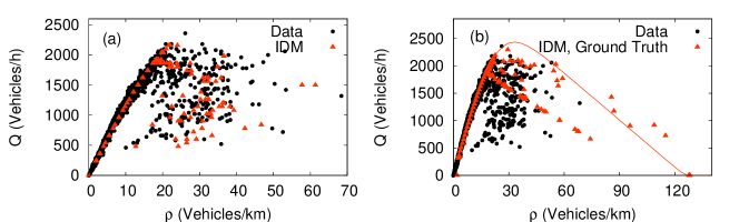
Figure 1: (a) Comparison of empirical and simulated flow-density data; (b) simulated ground truth for the density with the modeled fundamental diagram (solid curve).

At first sight, flow-density data seem to be useful for representing traffic instabilities since oscillations are non-stationary phenomena in which traffic is clearly out of equilibrium. This should lead to a wide scattering in the flow-density data of congested traffic (Kerner and Rehborn, 1996) as shown in Fig. 1 regardless of the theoretical question whether traffic flow has a definite equilibrium relation (“fundamental diagram”), or not (Nishinari et al., 2003; Kerner, 2004; Treiber et al., 2010a).

In fact, simulations with the Intelligent Driver Model (Treiber et al., 2000), as well as with a wide variety of other models, show wide scattering even for identical drivers and vehicles (Fig. 1). Nevertheless, flow-density data cannot be used for a quantitative calibration since other effects such as inter-driver variability (heterogeneous traffic) (Banks, 1999; Ossen et al., 2007; Treiber and Helbing, 1999), intra-driver variability (drivers change their behavior over time) (Treiber and Helbing, 2003), and many effects related to lane changes and platoons (Nishinari et al., 2003; Treiber et al., 2006b) may lead to wide scattering as well.

Moreover, since the density is not directly measurable by stationary detectors, it must be estimated, typically by making use of the hydrodynamic relation “flow divided by the average velocity”. The available temporal average, however, systematically underestimates the true spatial average relevant for this relation which results in an extreme bias in the flow-density data of congested traffic (Leutzbach, 1988; Helbing, 2001). Figure 1 illustrates this by means of simulations with the Intelligent Driver Model by Treiber et al. (2000)). This model has been calibrated such that the aggregated virtual detector shows a similar scattering as the empirical data (Fig. 1(a)). Plotting the same data points using the true spatial density (which, of course, is available in the simulation) reveals the systematic errors (Fig. 1(b)).

Alternatively, detailed information can be extracted from single-vehicle data, floating-car data, or trajectory data. However, since oscillations are collective phenomena, the high level of detail is not necessary. Moreover, to date, the availability of these data types is still limited, or the data are not suitable for our purposes. Specifically, the NGSIM trajectory data (US Department of Transportation, 2007) widely used as a testbed for these types of data cover road sections of typically 2 km in length while stop-and-go waves develop on typical scales of 5-10 km.

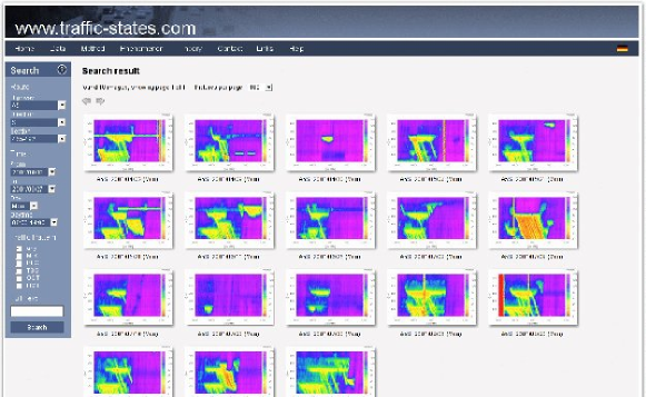
Figure 2: Screenshot of a publicly available image database of congestions on the German freeway A5. The database can be searched by criteria such as direction of travel, space interval, time interval, weekday, cause of the congestion, or the type of traffic pattern. In the example, the database has been filtered for jams occurring on Mondays in the southern driving direction. The images have been produced using a dedicated reconstruction technique (Treiber et al., 2010b).

In contrast, speed time series obtained from aggregated stationary detector data are widely available (see Fig. 2) and thus suitable for systematic calibration and benchmarking purposes. Moreover, since temporal averages are the appropriate mean when analyzing time series, no systematic errors arise. Using this type of data, the wavelength and propagation velocities of oscillations on freeways has been investigated by Lindgren (2005); Bertini and Leal (2005); Ahn and Cassidy (2007); Schönhof and Helbing (2007); Wilson (2008b) and compared for several countries by Zielke et al. (2008). However, the proposed schemes are not suitable for a systematic automated analysis. Moreover, to our knowledge, there seem to be no published work quantitatively determining the growth rate of the oscillations.

In this paper, we propose a systematic approach for calibrating and validating key features of traffic instabilities based on speed time series obtained from aggregated stationary detector data. This includes the propagation velocity, the wavelength, and the growth rate of the oscillations. We give first results based on a historic congestion database of the German freeway A5, and show that the method has a high discriminative power in assessing the model quality.

The proposed criteria are described in Sec. 2, and applied to observed data in Sec. 3. A first application to traffic flow models is given in Sec. 4 before Sec. 5 concludes with a discussion and an outlook.

2 The Proposed Quality Measures

The formulation of the criteria is based on qualitative empirical findings (“stylized facts”) (Treiber et al., 2010a) that are persistently observed on various freeways all over the world, e.g., the USA, Great Britain, the Netherlands, and Germany (Lindgren, 2005; Bertini and Leal, 2005; Ahn and Cassidy, 2007; Schönhof and Helbing, 2007; Zielke et al., 2008; Helbing et al., 2009; Wilson, 2008a). For our purposes, the relevant stylized facts are the following:

1. Congestion patterns are typically caused by bottlenecks which may be caused, e.g., by intersections, accidents, or gradients. Analyzing about 400 congestion patterns on the German freeways A5-North and A5-South (Fig. 2) did not bring conclusive evidence of a single breakdown without a bottleneck (Schönhof and Helbing, 2007).

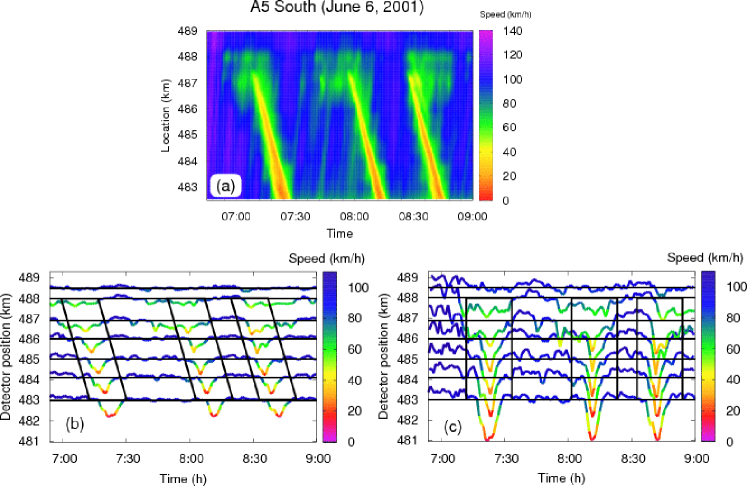
Figure 4: Stationary detector data displaying the evolution of isolated stop-and-go waves caused by a weak bottleneck located at about 487.5 km. (a) The spatiotemporal speed field, (b) the time series, and (c) the time series with skewed time axis are derived from the data as in Fig. 3. The parameters of the skewed time transformation $t^{\prime}=t-(x-x_{1})/c_{\text{cong}}$ are given by $x_{1}=483\,\mathrm{km}$ and $c_{\text{cong}}=-16\,\mathrm{km/h}$.

2. The congestion pattern can be localized or spatially extended. Localized patterns, as well as the downstream boundary of extended congestions, are either pinned at the bottleneck, or moving upstream at a characteristic velocity $c_{\rm cong}$. Only extended patterns (Fig. 3) and moving localized patterns (isolated stop-and-go waves, Fig. 4) are relevant for our investigation.

3. Most extended traffic patterns exhibit internal oscillations propagating upstream approximately at the same characteristic velocity $c\approx c_{\rm cong}=\text{const}$ (Daganzo, 2002; Mauch and Cassidy, 2002). In spatiotemporal representations such as that of Fig. 4 this corresponds to nearly parallel structures. For free traffic, the propagation velocity $c$ is somewhat lower than the average vehicle speed $\overline{V}$.

4. The amplitude of the oscillations increases while propagating upstream (Bertini and Leal, 2005; Ahn and Cassidy, 2007). We quantify this by defining a temporal growth rate $\sigma$ characterizing the growth process before saturation.

5. The average wavelength $L$ of the (saturated) waves increases with decreasing bottleneck strength (Treiber et al., 2000, 2010a).

In formulating the calibration criteria, We use the first two facts to filter the input data for applicable spatiotemporal regions (Sec. 2.2) while the quantities $c$, $\sigma$, and $L$ quantifying the remaining stylized facts constitute the criteria itself (Sections 2.4-2.6). In general, $c$, $\sigma$, and $L$ depend on the bottleneck strength which, therefore, needs to be quantitatively defined as well (Sec. 2.3).

2.1 Data Description

We assume that aggregated data for the flow $Q$ and speed $V$ (arithmetic average) are available from several detector cross sections at locations $i$. The distance between two adjacent detectors should not exceed about 2.5 km which generally is satisfied on relevant freeway sections (i.e., sections where traffic breakdowns are observed regularly). Usually, the flow and speed data $(V_{ilt},Q_{ilt})$ of cross section $i$ are available for each lane (index $l$) after each time interval (index $t$). With few exceptions, congested traffic is “synchronized” between lanes, i.e., the average speed at a given location and time is not significantly different across the lanes. We therefore use the following weighted averages as input for our calibration criteria:

$$V_{it}=\frac{1}{Q_{it}}\sum_{l=1}^{n_{i}}Q_{ilt}V_{ilt}$$ (1)

where $n_{i}$ is the number of mainroad lanes at location $i$. The total flow is given by

$$Q_{it}=\sum_{l=1}^{n_{i}}Q_{ilt}.$$ (2)

2.2 Filtering Spatiotemporal Regions

In order to determine the dynamic quantities $c$, $\sigma$, and $L$ from the input data $\{V_{it}\}$ it is necessary to restrict the spatiotemporal range to regions of actual congestions. From the stylized facts above, we use the information that the downstream boundary of congestions is either stationary at a bottleneck, or moving with a constant velocity $c_{\text{cong}}$. Furthermore, internal structures move at nearly the same velocity. This leads to defining parallelogram-shaped regions for both isolated stop-and-go waves, and extended congestions (cf. Figs. 4 and 3). The parallelogram is defined as follows:

• Two edges correspond to detector locations. The downstream edge is defined by the detector that is nearest to the bottleneck (in upstream direction). The upstream edge is at the detector location where the waves begin to saturate. This should include $n\geq 3$ detector cross sections. In the following, we will count the cross sections in the direction of the flow, i.e., the upstream edge is located at $x_{1}$, and the downstream edge at $x_{n}$.

• The other two edges are angled such that, in the spatiotemporal picture, the waves propagate parallel to these edges.

• The vertices $(x_{1},t_{1}^{\text{beg}})$ and $(x_{1},t_{1}^{\text{ end}})$ connected by the upstream edge are defined such that the parallelogram has a maximum area subject to the condition that there is no free traffic inside:

  $$t_{1}^{\text{beg}} = \max\limits_{i}\left(\hat{t}_{i}-\frac{x_{i}-x_{1}}{c_{\text{cong}}}\right),$$ (3)

  $$t_{1}^{\text{ end}} = \min\limits_{i}\left(\tilde{t}_{i}-\frac{x_{i}-x_{1}}{c_{\text{cong}}}\right):=t_{1}^{\text{beg}}+T\,.$$ (4)

  Here, $\hat{t}_{i}$ is the time where the aggregated speed time series $V_{it}$ of cross section $i$ drops below a critical speed $v_{c}$, and $\tilde{t}_{i}$ is the time where it rises above $v_{c}$. To reduce the occurrence of false signals, the time series can be smoothed over time scales of a few minutes just for this step. A value $v_{c}=70\,\mathrm{km/h}$ turned out to give good results for freeways.

2.3 Quantifying the Bottleneck Strength

For extended congestions, the quantities $c$, $\sigma$, and $L$ depend on the bottleneck strength. Therefore, this exogenous variable has to be characterized by the measured quantities as well. Theoretically, the bottleneck strength is defined by a local drop of the capacity that is available for the mainroad traffic (Schönhof and Helbing, 2007). However, this quantity is problematic to measure, particularly, if the bottleneck includes merging/diverging traffic (e.g., junctions, intersections, or lane closings). Therefore, we use as proxy the average vehicle speed at the detector nearest to the bottleneck,

$$\overline{V}=\frac{1}{T+1}\sum\limits_{t=t_{1}^{\text{beg}}+\Delta t}^{t_{1}^{\text{ end}}+\Delta t}V_{nt},\quad\Delta t=\frac{x_{n}-x_{1}}{c_{\text{cong}}}.$$ (5)

At this location, the oscillations inside extended jams are minimal (Stylized Fact 4) making $\overline{V}$ a well-defined quantity. In order to plot the characteristic quantities of isolated stop-and-go waves into the same diagram, such as Fig. 5, we define $\overline{V}$ as the speed outside of the wave, for this case.

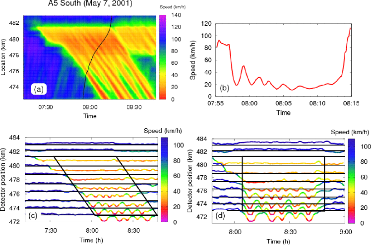
Figure 3: Example of stationary detector data displaying the development of stop-and-go waves from stationary congested traffic near the bottleneck. (a) Reconstruction of the spatiotemporal evolution of local vehicle speeds using a dedicated reconstruction technique (Treiber et al., 2010b). Also shown is a reconstructed vehicle trajectory (black curve). (b) Speed-time series of the reconstructed trajectory. (c) Speed-time series according to Eq. (1). The locations of the respective detectors are given by the black baselines, and the speed (reference value 90 km/h) is plotted relative to the baseline. The black parallelogram encloses the relevant spatiotemporal range defined in Sec. 2.2. (d) Representation of the same data with a skewed time axis $t^{\prime}=t-(x-x_{1})/c_{\text{cong}}$ with $x_{1}=473\,\mathrm{km}$ and $c_{\text{cong}}=-16\,\mathrm{km/h}$.

2.4 Propagation Velocity

The propagation velocity $c$ can be calculated by maximizing the sum of cross-correlation functions of speed time series of detector pairs $\{i,j\}$ in the congested region (at positions $x_{i}$ and $x_{j}$, respectively), with respect to the velocity $c$ (Coifman and Wang, 2005; Zielke et al., 2008):

$$c=\text{arg}\,\max_{c^{\prime}}\sum\limits_{i}\sum\limits_{j>i}\text{Corr}\left[V_{i}(t),V_{j}\left(t+\frac{x_{i}-x_{j}}{c^{\prime}}\right)\right],$$ (6)

where the continuous-in-time function $V_{i}(t)$ is defined by a piecewise linear interpolation of the detector time series $V_{it}$. Stylized Fact 3 suggests that the values of $c$ lie in a very small range which is confirmed by Fig. 5(d). This makes it possible to define the spatiotemporal region using the a-priori estimate $c_{\text{cong}}$ without danger of circular reasoning. When selecting spatiotemporal regions of free traffic, Eq. (6) can be used to determine the propagation velocity of perturbations in free traffic (data points at the upper right corner of Fig. 5(d)).

2.5 Growth rate

The average spatial growth rate $\tilde{\sigma}$ of perturbations is defined in terms of the slope of the linear regression of the logarithm of the amplitude,

$$\tilde{\sigma}=\frac{\sum_{i}x_{i}\ln|A_{i}|-n\overline{x}\,\overline{\ln|A_{i}|}}{\sum_{i}x_{i}^{2}-n\overline{x}^{2}},$$ (7)

where the amplitude $A_{i}$ is approximated by the standard deviation of the speed time series $V_{it}$ inside the parallelogram. Of course, $\tilde{\sigma}$ is only a rough approximation of the true growth rate. Particularly, $\tilde{\sigma}$ is influenced by non-collective fluctuations caused by random noise and driver-vehicle heterogeneity as well as by saturation effects, particularly, if the spatiotemporal region is not defined carefully. Both effects systematically decrease the estimated growth rate but do not invalidate the overall picture. However, it is essential to calculate the simulated quantities using exactly the same measuring and estimation procedures.

Once the spatial growth rate is known, the temporal growth rate is given by

$$\sigma=c\tilde{\sigma}.$$ (8)

Notice that, in general, $\tilde{\sigma}$ is negative, and $\sigma$ positive.

2.6 Wavelength

The average period $\tau$ of the oscillations of extended congestions is given by the position of the first nontrivial peak of the autocorrelation functions of detector time series inside the parallelogram. In some cases, waves merge during their propagation such that the period and the wavelength increases with the distance from the bottleneck. We therefore define $\tau$ at a certain development stage, namely at the limit of saturation:

$$\tau=\text{arg}\,\max_{\tau^{\prime}>0}\,\text{Corr}\left[V_{1}(t),V_{1}(t+\tau^{\prime})\right].$$ (9)

In analogy to Eq. (8), the associated wavelength is given by

$$L=|c|\tau.$$ (10)

3 Application to Freeway Data

The characteristic quantities defined in the previous section have been calculated for about 30 instances of traffic congestions observed on a section of the German freeway A5-South near Frankfurt for April and May 2001. Images of the corresponding spatiotemporal speed fields can be viewed at www.traffic-states.com (cf. Fig. 2 for a screenshot). Not all of the more than 60 jams observed in the southern direction in this time period are suited for the analysis: Localized jams must be moving (filter criterion “MLC”), and extended jams must exhibit distinct oscillating structures (filter criteria “OCT” or “TSG”). Additionally, they must be sufficiently extended such that the parallelogram includes at least three cross sections, and each cross section records at least three oscillations. While oscillating structures are observed for most of the cases except for very strong or weak bottlenecks (filter criteria “HCT” and “HST”, respectively), nearly 50 % of the remaining candidates do not satisfy the minimum size criteria.

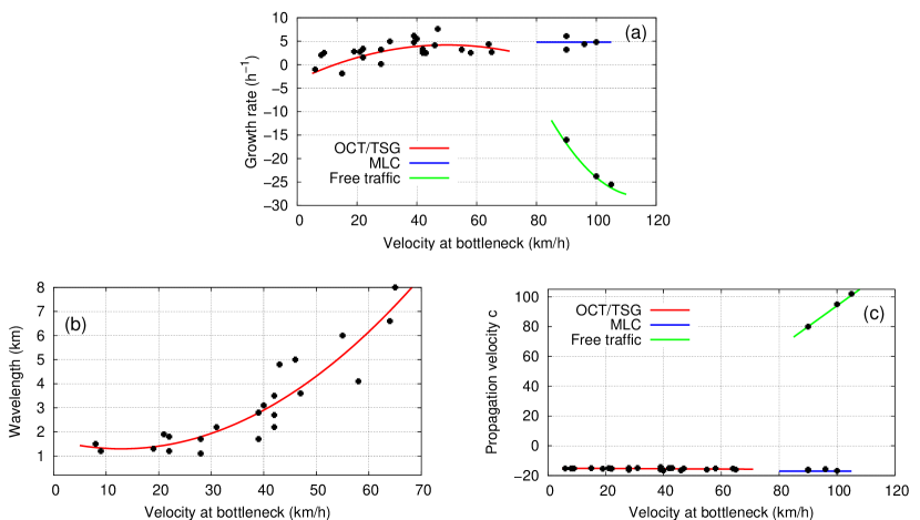
Figure 5: Characteristic properties of the propagation of perturbations in congested traffic. (a) Growth rate $\sigma$, (b) wavelength $L$, and (c) propagation velocity $c$, as a function of the average speed $\overline{V}$ characterizing the bottleneck strength.

Figure 5 displays the main result which can be used not only for calibration purposes, but also for understanding the traffic dynamics in general. Part (a) of this figure shows the growth rate of the moving structures inside extended congestions (points for $\overline{V}$ below 70 km/h), the growth rate of isolated stop-and-go waves (MLC, top right corner), and, for comparison, the growth rate of some moving structures in free traffic. For congested traffic, the growth rate is generally positive, apart for very low average velocities $\overline{V}$ corresponding to extended congestions behind strong bottlenecks (usually accident-caused lane closures, selected in the database by the criterium “accident”). This positive growth rate can be directly experienced by the driver (or alternatively obtained from floating-car data) as shown in Fig. 3(b): When approaching the bottleneck , the experienced velocity oscillations apparently decrease in amplitude with the growth rate

$$\sigma_{\text{FC}}=\overline{V}_{\text{FC}}\tilde{\sigma}.$$ (11)

They have the apparent period

$$\tau_{\text{FC}}=\tau\left(\frac{|c|}{|c|+\overline{V}_{\text{FC}}}\right)$$ (12)

where $\overline{V}_{\text{FC}}$ is the average speed of the floating car.

Figure 5(b) shows that the wavelength decreases with increasing bottleneck strength, but always remains above 1 km. Finally, Fig 5(c) confirms that the propagation velocity is nearly constant (in the range $-17\,\mathrm{km/h}$ to $-16\,\mathrm{km/h}$ for extended jams and about $-18\,\mathrm{km/h}$ for isolated moving waves).

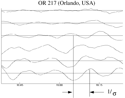
Figure 6: Speed-time series of several detectors on the US American freeway OR 217 (Zielke et al., 2008). Shown are deviations (oscillating curves) from the average speed (horizontal baselines). The detector spacings are proportional to the spacings of the baselines. Also shown is the time period $1/\sigma$ in which the amplitudes of each wave increase by a factor of $e$.

The analysis quantitatively confirms the stylized facts presented in Sec. 2. Particularly, there is no empirical evidence against the existence of linear instabilities in congested traffic. This is also confirmed by data from other freeways in several countries, although there are quantitative deviations (this, exactly, is the basis for calibrating the models). As an example, Fig. 6 taken from Zielke et al. (2008) shows speed time series which are suitable for the present analysis. The growth rate is comparable to the A5 data while the propagation velocity $c\approx-20\,\mathrm{km/h}$ has a somewhat higher absolute value (Zielke et al., 2008) .

4 A First Test of Traffic Flow Models

In this section, we will show how the results can be applied to calibrating the dynamic aspects of traffic flow models by testing the Intelligent-Driver Model (IDM) (Treiber et al., 2000) and the Human Driver Model (HDM) (Treiber et al., 2006a) on the extended congestion shown in Fig. 3. Both models are time-continuous car-following models, but the calibration procedures can be applied as well to discrete-in-time models, cellular automata and to macroscopic models.

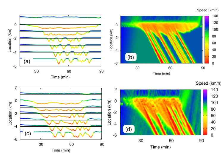
Figure 7: Examples of simulated virtual detector data based on simulations with the Intelligent Driver Model for a permanent bottleneck (plots a and b), and the Human Driver Model with a temporary bottleneck (c, d). The simulated data aggregation (time intervals of 1 min), and the transformations to display the data are the same as for the empirical data in Fig. 3.

In the simulations, the bottleneck is represented by an on-ramp. The on-ramp flow, i.e., the bottleneck strength, is chosen such that the average velocity $\overline{V}$ near the bottleneck, Eq. 5, is consistent with the data. At $t=70\,\mathrm{min}$, the bottleneck is reduced resulting in a moving downstream front of the congestion at later times (this has no influence on the calibration results). Virtual detectors are positioned every kilometer, and vehicle passage times and speeds are aggregated in one-minute intervals, in analogy to the data sampling at the real detectors. The result is displayed in Fig. 7.

The criteria for the actual calibration and assessment are the propagation velocity $c$, wavelength $L$ (or period $\tau$), and growth rate $\sigma$. They are calculated from the virtual detector data with exactly the same scheme that has been used for the real data. Since the speed $\overline{V}$, i.e., the bottleneck strength, is fixed, there are no degrees of freedom by manipulating the bottleneck. A comparison with the empirical values $\sigma_{\text{obs}}=5\,\mathrm{h^{-1}}$, $c_{\text{obs}}=-17\,\mathrm{km/h}$, and $\tau_{\text{obs}}=10\,\mathrm{min}$ (cf. Fig. 3) gives a first impression of the discriminative power of the proposed calibration and testing method: The empirical propagation velocity $c$ agrees with both models. However, for the IDM simulation, the period $\tau_{\text{IDM}}=6\,\mathrm{min}$ of the waves is too short, and the growth rate $\sigma_{\text{IDM}}\approx 10\,\mathrm{h^{-1}}$ (calculated using the detectors at 0, 1, and 2 km) is too high. It turns out that this cannot be improved significantly by changing the model parameters, i.e., calibrating the model. For the HDM simulation, the period $\tau_{\text{HDM}}=8\,\mathrm{min}$ deviates less, and the growth rate $\sigma_{\text{HDM}}\approx 5\,\mathrm{h^{-1}}$ is consistent with the data. Since, in contrast to the IDM, the HDM includes explicit reaction times and multi-anticipation (the drivers take into account multiple leaders), this may mean that both aspects are essential for a quantitative modelling. However, it is too early to draw definitive conclusions.

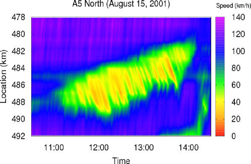
Figure 8: A moving bottleneck filtered from the image database www.traffic-states.com: Validating a model with data it most probably has never seen before.

5 Discussion and Outlook

In conclusion, we propose three aspects of traffic instabilities that are accessible to a systematic and quantitative test of model prediction: the wavelength, the propagation velocity, and the growth rate. Since all properties are functions of the average velocity indicating the bottleneck strength, there should be enough input for a discriminative testing of models. All quantities are defined in terms of automated schemes enabling the systematic investigation of large-scale data bases. As a first step, it is planned to investigate the complete database displayed at www.traffic-states.com containing more than 400 instances of congestions.

The database contains also some unusual patterns to which the scheme of Sec. 2 can be easily generalized and which may be used to validate the predictive power of models calibrated to the more conventional patterns discussed above. For example, there are some searchable instances of “moving bottlenecks” (Fig. 8), possibly caused by very slow special transports or obstructions due to “moving road works” (such as mowing the median lawn).

We notice that all proposed quantities for calibrating and testing relate to existing congestions. Due to the stochastic nature of the perturbations eventually leading to a breakdown, predictions for an actual breakdown are necessarily restricted to a probabilistic level (Elefteriadou et al., 1995; Brilon et al., 2005).

It must be emphasized that calibrations based on microscopic quantities such as the difference between measured and simulated gaps are strongly influenced by unpredictable intra- and inter-driver variations (Ossen et al., 2007; Kesting and Treiber, 2008) resulting in little discriminative power (Brockfeld et al., 2004; Ranjitkar et al., 2004; Ossen and Hoogendoorn, 2005; Punzo and Simonelli, 2005). However, when calibrating against integrated quantities such as the traveling time (Brockfeld et al., 2003), important aspects such as accelerations or the properties of oscillations are averaged away resulting in reduced discriminative power as well. In contrast, the schemes proposed here probe the traffic dynamics on the intermediate scale of individual oscillations which is of the order of one kilometer and a few minutes. Since we probe on collective phenomena, inter- and intra-driver variabilities should only play a minor role. However, the scale is sufficiently microscopic to retain accelerations. We therefore expect that the proposed schemes can be applied to a better and more discriminative benchmarking of microscopic and macroscopic models with respect to traffic instabilities. This is the topic of ongoing work.

Acknowledgements

The authors would like to thank the Hessisches Landesamt für Straßen- und Verkehrswesen for providing the freeway data.

References

- Ahn and Cassidy (2007) Ahn, S., Cassidy, M. J., 2007. Freeway traffic oscillations and vehicle lane-change maneuvers. In: Allsop, R. E., Bell, M. G. H., Heydecker, B. G. (Eds.), Transportation and Traffic Theory 2007. Elsevier, Ch. 29, pp. 691–710.
- Banks (1999) Banks, J. H., 1999. An investigation of some characteristics of congested flow. Transportation Research Record 1678, 128–134.
-
Bertini and Leal (2005)
Bertini, R. L., Leal, M. T., 2005. Empirical study of traffic features at a
freeway lane drop. Journal of Transportation Engineering 131 (6), 397–407.
URL http://link.aip.org/link/?QTE/131/397/1 - Brilon et al. (2005) Brilon, W., Geistefeldt, J., Regler, M., 2005. Transportation and Traffic Theory: Flow, Dynamics and Human Interaction. Proceedings of the 16th International Symposium on Transportation and Traffic Theory. Elsevier, Ch. Reliability of freeway traffic flow: a stochastic concept of capacity, pp. 125–144.
- Brockfeld et al. (2003) Brockfeld, E., Kühne, R. D., Skabardonis, A., Wagner, P., 2003. Toward benchmarking of microscopic traffic flow models. Transportation Research Record 1852, 124–129.
- Brockfeld et al. (2004) Brockfeld, E., Kühne, R. D., Wagner, P., 2004. Calibration and validation of microscopic traffic flow models. Transportation Research Record 1876, 62–70.
- Coifman and Wang (2005) Coifman, B. A., Wang, Y., 2005. Average velocity of waves propagating through congested freeway traffic. In: Mahmassani, H. S. (Ed.), Transportation and Traffic Theory: Flow, Dynamics and Human Interaction. Elsevier, pp. 165–179.
- Daganzo (2002) Daganzo, C. F., 2002. A behavioral theory of multi-lane traffic flow. part I: Long homogeneous freeway sections. Transportation Research Part B: Methodological 36 (2), 131–158.
- Elefteriadou et al. (1995) Elefteriadou, L., Roess, R., McShane, W., 1995. Probabilistic nature of breakdown at freeway merge junctions. Transportation Research Record 1484, 80–89.
- Helbing (2001) Helbing, D., 2001. Traffic and related self-driven many-particle systems. Reviews of Modern Physics 73, 1067–1141.
- Helbing et al. (2009) Helbing, D., Treiber, M., Kesting, A., Schönhof, M., 2009. Theoretical vs. empirical classification and prediction of congested traffic states. The European Physical Journal B 69, 583–598.
- Hoogendoorn and Bovy (2001) Hoogendoorn, S., Bovy, P., 2001. State-of-the-art of vehicular traffic flow modelling. Proceedings of the Institution of Mechanical Engineers, Part I: Journal of Systems and Control Engineering 215 (4), 283–303.
- Kerner and Rehborn (1996) Kerner, B., Rehborn, H., 1996. Experimental properties of complexity in traffic flow. Physical Review E 53, R4275–R4278.
- Kerner (2004) Kerner, B. S., 2004. The Physics of Traffic: Empirical Freeway Pattern Features, Engineering Applications, and Theory. Springer.
- Kesting and Treiber (2008) Kesting, A., Treiber, M., 2008. Calibrating car-following models by using trajectory data: Methodological study. Transportation Research Record 2088, 148–156.
- Leutzbach (1988) Leutzbach, W., 1988. Introduction to the Theory of Traffic Flow. Springer, Berlin.
- Lindgren (2005) Lindgren, R., 2005. Analysis of Flow Features in Queued Traffic on a German Freeway. Ph.D. thesis, Portland State University.
- Mauch and Cassidy (2002) Mauch, M., Cassidy, M. J., 2002. Freeway traffic oscillations: observations and predictions. In: Taylor, M. A. (Ed.), Transportation and traffic theory in the 21st century: Proceedings of the Symposium of Traffic and Transportation Theory. Elsevier, pp. 653–672.
- Nishinari et al. (2003) Nishinari, K., Treiber, M., Helbing, D., 2003. Interpreting the wide scattering of synchronized traffic data by time gap statistics. Physical Review E 68, 067101.
- Ossen and Hoogendoorn (2005) Ossen, S., Hoogendoorn, S. P., 2005. Car-following behavior analysis from microscopic trajectory data. Transportation Research Record 1934, 13–21.
- Ossen et al. (2007) Ossen, S., Hoogendoorn, S. P., Gorte, B. G., 2007. Inter-driver differences in car-following: A vehicle trajectory based study. Transportation Research Record 1965, 121–129.
- Pipes (1953) Pipes, L., 1953. An operational analysis of traffic dynamics. Journal of Applied Physics 24, 274.
- Punzo and Simonelli (2005) Punzo, V., Simonelli, F., 2005. Analysis and comparision of microscopic flow models with real traffic microscopic data. Transportation Research Record 1934, 53–63.
- Ranjitkar et al. (2004) Ranjitkar, P., Nakatsuji, T., Asano, M., 2004. Performance evaluation of microscopic flow models with test track data. Transportation Research Record 1876, 90–100.
- Reuschel (1950) Reuschel, A., 1950. Fahrzeugbewegungen in der Kolonne. Österreichisches Ingenieur-Archiv 4, 193–215.
- Schönhof and Helbing (2007) Schönhof, M., Helbing, D., 2007. Empirical features of congested traffic states and their implications for traffic modeling. Transportation Science 41, 1–32.
- Treiber and Helbing (1999) Treiber, M., Helbing, D., 1999. Macroscopic simulation of widely scattered synchronized traffic states. Journal of Physics A: Mathematical and General 32 (1), L17–L23.
- Treiber and Helbing (2003) Treiber, M., Helbing, D., 2003. Memory effects in microscopic traffic models and wide scattering in flow-density data. Physical Review E 68, 046119.
- Treiber et al. (2000) Treiber, M., Hennecke, A., Helbing, D., 2000. Congested traffic states in empirical observations and microscopic simulations. Physical Review E 62, 1805–1824.
- Treiber et al. (2006a) Treiber, M., Kesting, A., Helbing, D., 2006a. Delays, inaccuracies and anticipation in microscopic traffic models. Physica A 360, 71–88.
- Treiber et al. (2006b) Treiber, M., Kesting, A., Helbing, D., 2006b. Understanding widely scattered traffic flows, the capacity drop, and platoons as effects of variance-driven time gaps. Physical Review E 74, 016123.
- Treiber et al. (2010a) Treiber, M., Kesting, A., Helbing, D., 2010a. Three-phase traffic theory and two-phase models with a fundamental diagram in the light of empirical stylized facts. Transportation Research Part B: Methodological 44, 983–1000.
- Treiber et al. (2010b) Treiber, M., Kesting, A., Wilson, R. E., 2010b. Reconstructing the traffic state by fusion of heterogenous data. Computer-Aided Civil and Infrastructure Engineering, preprint arxiv.org/abs/0909.4467, in press.
- Treiterer and Myers (1974) Treiterer, J., Myers, J., 1974. The hysteresis phenomenon in traffic flow. In: Buckley, D. (Ed.), Proc. 6th Int. Symp. on Transportation and Traffic Theory. Elsevier, New York, p. 13.
- US Department of Transportation (2007) US Department of Transportation, 2007. NGSIM – Next Generation Simulation. http://www.ngsim.fhwa.dot.gov.
- Wilson (2008a) Wilson, R., 2008a. Mechanisms for spatio-temporal pattern formation in highway traffic models. Philosophical Transactions of the Royal Society A 366 (1872), 2017–2032.
- Wilson (2008b) Wilson, R. E., 2008b. From inductance loops to vehicle trajectories. In: Symposium on the Fundamental Diagram: 75 Years (Greenshields 75 Symposium). Transportation Research Board.
- Zielke et al. (2008) Zielke, B., Bertini, R., Treiber, M., 2008. Empirical Measurement of Freeway Oscillation Characteristics: An International Comparison. Transportation Research Record 2088, 57–67.