Homotopical Complexity of 2D Billiard Orbits

Abstract.

Traditionally, rotation numbers for toroidal billiard flows are defined as the limiting vectors of average displacements per time on trajectory segments. Naturally, these creatures live in the (commutative) vector space $\operatorname{\mathbb{R}}^{n}$, if the toroidal billiard is given on the flat $n$-torus. The billiard trajectories, being curves, often getting very close to closed loops, quite naturally define elements of the fundamental group of the billiard table. The simplest non-trivial fundamental group obtained this way belongs to the classical Sinai billiard, i.e. the billiard flow on the 2-torus with a single, strictly convex obstacle (with smooth boundary) removed. This fundamental group is known to be the group $\textbf{F}_{2}$ freely generated by two elements, which is a heavily noncommutative, hyperbolic group in Gromov’s sense. We define the homotopical rotation number and the homotopical rotation set for this model, and provide lower and upper estimates for the latter one, along with checking the validity of classically expected properties, like the density (in the homotopical rotation set) of the homotopical rotation numbers of periodic orbits.

The natural habitat for these objects is the infinite cone erected upon the Cantor set $\text{Ends}(\textbf{F}_{2})$ of all “ends” of the hyperbolic group $\textbf{F}_{2}$. An element of $\text{Ends}(\textbf{F}_{2})$ describes the direction in (the Cayley graph of) the group $\textbf{F}_{2}$ in which the considered trajectory escapes to infinity, whereas the height function $t$ ($t\geq 0$) of the cone gives us the average speed at which this escape takes place.

The main results of this paper claim that the orbits can only escape to infinity at a speed not exceeding $\sqrt{2}$, and any direction $e\in\text{Ends}(F_{2})$ for the escape is feasible with any prescribed speed $s$, $0\leq s\leq\sqrt{2}/2$. This means that the radial upper and lower bounds for the rotation set $R$ are actually pretty close to each other.

1. Introduction

The concept of rotation number finds its origin in the study of the average rotation around the circle $S^{1}$ per iteration, as classically defined by H. Poincaré in the 1880’s, when one iterates an orientation-preserving circle homeomorphism $f:S^{1}\rightarrow S^{1}$. This is equivalent to studying the average displacement $(1/n)(F^{n}(x)-x)$ ($x\in\operatorname{\mathbb{R}}$) for the iterates $F^{n}$ of a lifting $F:\operatorname{\mathbb{R}}\rightarrow\operatorname{\mathbb{R}}$ of $f$ on the universal covering space $\operatorname{\mathbb{R}}$ of $S^{1}$. The study of fine homotopical properties of geodesic lines on negatively curved, closed surfaces goes back at least to Morse [Mor24]. As far as we know, the first appearance of the concept of homological rotation vectors (associated with flows on manifolds) was the paper of Schwartzman [Sch57], see also Boyland [Boy00] for further references and a good survey of homotopical invariants associated with geodesic flows. Following an analogous pattern, in [BMS06] we defined the (still commutative) rotation numbers of a $2D$ billiard flow on the billiard table $\mathbb{T}^{2}=\operatorname{\mathbb{R}}^{2}/\operatorname{\mathbb{Z}}^{2}$ with one convex obstacle (scatterer) $\mathcal{O}$ removed. Thus, the billiard table (configuration space) of the model in [BMS06] was $\mathcal{Q}=\mathbb{T}^{2}\setminus\mathcal{O}$. Technically speaking, we considered trajectory segments $\{x(t)|0\leq t\leq T\}\subset\mathcal{Q}$ of the billiard flow, lifted them to the universal covering space $\operatorname{\mathbb{R}}^{2}$ of $\mathbb{T}^{2}$ (not of the configuration space $\mathcal{Q}$), and then systematically studied the rotation vectors as limiting vectors of the average displacement $(1/T)(\tilde{x}(T)-\tilde{x}(0))\in\operatorname{\mathbb{R}}^{2}$ of the lifted orbit segments $\{\tilde{x}(t)|0\leq t\leq T\}$ as $T\rightarrow\infty$. These rotation vectors are still “commutative”, for they belong to the vector space $\operatorname{\mathbb{R}}^{2}$.

Despite all the advantages of the homological (or “commutative”) rotation vectors (i. e. that they belong to a real vector space, and this provides us with useful tools to construct actual trajectories with prescribed rotational behaviour), in our current view the “right” lifting of the trajectory segments $\{x(t)|0\leq t\leq T\}\subset\mathcal{Q}$ is to lift these segments to the universal covering space of $\mathcal{Q}=\mathbb{T}^{2}\setminus\mathcal{O}$, not of $\mathbb{T}^{2}$. This, in turn, causes a profound difference in the nature of the arising rotation “numbers”, primarily because the fundamental group $\pi_{1}(\mathcal{Q})$ of the configuration space $\mathcal{Q}$ is the highly complex group $\textbf{F}_{2}$ freely generated by two generators (see section 2 below or [Mas91]). After a bounded modification, trajectory segments $\{x(t)|0\leq t\leq T\}\subset\mathcal{Q}$ give rise to closed loops $\gamma_{T}$ in $\mathcal{Q}$, thus defining an element $g_{T}=[\gamma_{T}]$ in the fundamental group $\pi_{1}(\mathcal{Q})=\textbf{F}_{2}$. The limiting behavior of $g_{T}$ as $T\rightarrow\infty$ will be investigated, quite naturally, from two viewpoints:

1. The direction “$e$” is to be determined, in which the element $g_{T}$ escapes to infinity in the hyperbolic group $\textbf{F}_{2}$ or, equivalently, in its Cayley graph $\mathcal{G}$, see section 2 below. All possible directions $e$ form the horizon or the so called ideal boundary $\text{Ends}(\textbf{F}_{2})$ of the group $\textbf{F}_{2}=\pi_{1}(\mathcal{Q})$, see [CP93].

2. The average speed $s=\lim_{T\rightarrow\infty}(1/T)\text{dist}(g_{T},1)$ is to be determined, at which the element $g_{T}$ escapes to infinity, as $T\rightarrow\infty$. These limits (or limits $\lim_{T_{n}\rightarrow\infty}(1/T_{n})\text{dist}(g_{T_{n}},1)$ for sequences of positive reals $T_{n}\nearrow\infty$) are nonnegative real numbers.

The natural habitat for the two limit data $(s,e)$ is the infinite cone

$$C=([0,\infty)\times\text{Ends}(\textbf{F}_{2}))/(\{0\}\times\text{Ends}(\textbf{F}_{2}))$$

erected upon the set $\text{Ends}(\textbf{F}_{2})$, the latter supplied with the usual Cantor space topology. Since the homotopical “rotation numbers” $(s,e)\in C$ (and the corresponding homotopical rotation sets) are defined in terms of the noncommutative fundamental group $\pi_{1}(\mathcal{Q})=\textbf{F}_{2}$, these notions will be justifiably called homotopical or noncommutative rotation numbers and sets.

In accordance with [BMS06], we will focus on systems with a so-called “small obstacle”, i.e., when the sole obstacle $\mathcal{O}$ is contained by some circular disk of radius less than $\sqrt{2}/4$. Furthermore, again following [BMS06], most of the time we will restrict our attention to the so-called admissible orbits, see the paragraph right after the proof of Lemma 2.5 in [BMS06]. The corresponding rotation set will be the so-called admissible homotopical rotation set $AR\subset C$. The homotopical rotation set $R$ defined without the restriction of admissibility will be denoted by $R$. Plainly, $AR\subset R$ and these sets are closed subsets of the cone $C$.

The main results of this paper are theorems 2.12 and 2.16. The former claims that the set $R$ is contained in the closed ball $B(0,\,\sqrt{2})$ of radius $\sqrt{2}$ centered at the vertex $0=\{0\}\times\text{Ends}(\textbf{F}_{2})$ of the cone $C$. In particular, both sets $AR$ and $R$ are compact. The latter result claims that the set $AR$ contains the closed ball $B(0,\sqrt{2}/2)$ of $C$, provided that the radius $r_{0}$ of the sole circular obstacle is less than $\sqrt{5}/10$. Thus, these two results provide a pretty detailed description of the homotopical complexity of billiard orbits: Any direction $e\in\text{Ends}(F_{2})$ is feasible for the trajectory to go to infinity, the speed of escape $s$ cannot be bigger than $\sqrt{2}$, whereas any speed $s$, $0\leq s\leq\sqrt{2}/2$, is achievable in any direction $e\in\text{Ends}(F_{2})$. Example 2.15 shows that, in sharp contrast with the expectations and the analogous results for the commutative rotation numbers in [BMS06], the star-shaped set $R$ is not contained in the unit ball $B(0,1)$ of $C$: it contains some radii of length $\sqrt{2}$, thus the upper estimate of Theorem 2.12, at least as a direction independent upper bound for the radial size of $R$, is actually sharp.

Finally, in the concluding Section 3 we present a corollary (Theorem 3.1) of the proofs of Section 2 and make a few remarks. The theorem provides an effective constant as an upper bound for the topological entropy $h_{top}(r_{0})$ of the billiard flow, where $r_{0}$ is the radius of the sole circular obstacle. The upper bound we obtain is explicit, unlike the one obtained in [BFK98] for the topological entropy of the flow.

Remark 3.6 asserts what is always expected for “decent” dynamical systems regarding the relation between homotopical rotation sets and periodic orbits: the homotopical rotation numbers of periodic admissible orbits form a dense subset in $AR$.

Finally, remarks 3.7–3.9 briefly outline the possibilities of some interesting follow-up research, namely the investigation and understanding of the homotopical rotation numbers for $2D$ toroidal billiards with $N$ round obstacles.

2. Main Results

Lower Estimate for the Homotopical Rotation Set

The configuration space $\mathcal{Q}$ (the billiard table) of our system is the punctured $2D$-torus $\mathcal{Q}=\mathbb{T}^{2}\setminus\mathcal{O}$, where the removed obstacle $\mathcal{O}$ is the open disk of radius $r_{0}$, $0<r_{0}<\sqrt{2}/4$, centered at the origin $(0,0)$. (For simplicity we assume that the obstacle is a round disk, though this is only an unimportant technical condition, see Remark 3.8 below.) The upper bound of $\sqrt{2}/4$ is exactly the condition of having a so-called “small obstacle” in the sense of [BMS06].

The fundamental group $\pi_{1}(\mathcal{Q})$ of $\mathcal{Q}$ is classically known to be the group $\textbf{F}_{2}=\langle a,b\rangle$, freely generated by the elements $a$ and $b$, see, for example, [Mas91]. Perhaps the simplest way to see this is to consider a simply connected fundamental domain

(2.1) $$\mathcal{Q} = \{x=(x_{1},x_{2})\in\operatorname{\mathbb{R}}^{2}|0\leq x_{1},x_{2}\leq 1,\ \text{dist}(x,\operatorname{\mathbb{Z}}^{2})\geq r_{0}\},$$

where the upper and lower horizontal sides of this domain are identified via the equivalence relation $(x_{1},0)\sim(x_{1},1)$, $r_{0}\leq x_{1}\leq 1-r_{0}$, and the left and right vertical sides are similarly identified via $(0,x_{2})\sim(1,x_{2})$ for $r_{0}\leq x_{2}\leq 1-r_{0}$.

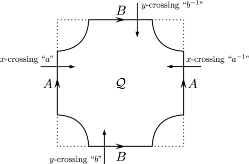
Figure 1.

The domain $\mathcal{Q}$ is obtained by identifying the opposite sides $A-A$ and $B-B$, just as the arrows indicate. This space is homeomorphic to the topological space that we obtain by gluing together two copies of a closed strip $S^{1}\times[-1,1]$ by identifying the rectangle $R_{1}=[-1/10,1/10]\times[-1,1]$ (in the first copy) with the same rectangle $R_{2}=R_{1}$ (in the second copy) via the map $(x,y)\mapsto(y/10,10x)$, $|x|\leq 1/10$, $|y|\leq 1$, see Fig. 2.

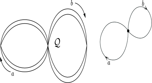
Figure 2.

The space $\mathcal{Q}$ is homotopically equivalent to the “bouquet” of two circles, see the right part of Fig. 2. The fundamental group of the latter space is classically known to be (see [Mas91]) the group $\textbf{F}_{2}=\langle a,b\rangle$ freely generated by two elements “$a$” and “$b$”, so that “$a$” corresponds to making a loop along the first circle (in some selected direction), whereas the generator “$b$” corresponds to making a similar loop along the other circle. Clearly, these two generators correspond to the so-called $x$- and $y$-crossings of curves (see Fig. 1). An $x$-crossing “$a$” occurs when a smooth curve $\gamma(t)=(\gamma_{1}(t),\gamma_{2}(t))$ intersects a line $\gamma_{1}(t)=k$ ($k\in\operatorname{\mathbb{Z}}$) with $\dot{\gamma_{1}}(t)>0$, while a $y$-crossing “$b$” takes place when $\gamma(t)=(\gamma_{1}(t),\gamma_{2}(t))$ intersects a line $\gamma_{2}(t)=k$ ($k\in\operatorname{\mathbb{Z}}$) with $\dot{\gamma_{2}}(t)>0$. The “inverse crossings” $a^{-1}$ and $b^{-1}$ occur when the corresponding derivatives are negative. We may assume that all these crossings are transversal. More precisely, we may restrict our studies to such curves.

Our general goal is to study the large scale behavior of “admissible” billiard orbit segments $\pi(x(t))=\pi((x_{1}(t),x_{2}(t)))$, $0\leq t\leq T$, $\text{dist}(x(0),(0,0))=r_{0}$, as $T\rightarrow\infty$. Here, “admissibility” is understood in the sense of [BMS06], which means the following: Denote by $\textbf{k}_{0},\textbf{k}_{1},\ldots,\textbf{k}_{n}\in\operatorname{\mathbb{Z}}^{2}$ the centers of the obstacles $\mathcal{O}_{\textbf{k}_{i}}$ at whose boundaries the lifted orbit segment $x(t)$, $0\leq t\leq T$, is reflected, listed in time order. Admissibility means that the following three conditions are satisfied:

1. $\textbf{k}_{0}=(0,0)$,

2. for any $1\leq i\leq n$, only the obstacles $\mathcal{O}_{\textbf{k}_{i-1}}$ and $\mathcal{O}_{\textbf{k}_{i}}$ intersect the convex hull of these two obstacles,

3. for any $1\leq i\leq n-1$, the obstacle $\mathcal{O}_{\textbf{k}_{i}}$ is disjoint from the convex hull of $\mathcal{O}_{\textbf{k}_{i-1}}$ and $\mathcal{O}_{\textbf{k}_{i+1}}$.

A crucial result of [BMS06], Theorem 2.2 claims the existence of orbits with any prescribed (finite or infinite) admissible itinerary $\left(\textbf{k}_{n}\right)_{n=N_{1}}^{N_{2}}$.

In this paper we always consider the obstacles to be closed, i.e., containing their boundaries. Whenever dealing with the so called admissible orbits, we shall restrict ourselves to studying only

1. special admissible billiard orbit segments, the so called strongly admissible orbit segments, for which the above discrete itinerary

   $$(\textbf{k}_{0},\textbf{k}_{1},\ldots,\textbf{k}_{n})$$

   has the additional property that $\text{dist}(\textbf{k}_{i-1},\textbf{k}_{i})\leq\sqrt{2}$ for $i=1,2,\ldots,n$.

We are primarily interested in discovering the asymptotic behavior of the above segments $\{\pi(x(t))|0\leq t\leq T\}$ from the viewpoint of the fundamental group $\pi_{1}(\mathcal{Q})$, as $T\rightarrow\infty$. The first question that arises here is how to measure the large-scale motion in $\pi_{1}(\mathcal{Q})$ that is naturally associated with $\{\pi(x(t))|0\leq t\leq T\}$? In order to answer this question, we first consider the so-called Cayley graph $\mathcal{G}=(\mathcal{V},\mathcal{E})$ of the group $\pi_{1}(\mathcal{Q})=\textbf{F}_{2}$ determined by the symmetric system of generators $\mathcal{A}=\{a,a^{-1},b,b^{-1}\}$. The vertex set $\mathcal{V}$ of the Cayley graph $\mathcal{G}$ is, by definition, the underlying set of the group $\textbf{F}_{2}$. We say that an oriented edge of type $l\in\mathcal{A}$ goes from the element $w_{1}\in\mathcal{V}$ to the element $w_{2}\in\mathcal{V}$ if $w_{1}l=w_{2}$. The arising oriented graph consists of pairs of oppositely oriented edges $l,l^{-1}$. Other than the these cycles of length 2, there are no cycles in the Cayley graph $\mathcal{G}$. If we identify the opposite edges, then, obviously, we obtain a tree in which every vertex has degree 4 (a so-called 4-regular tree). The graph $\mathcal{G}$ is considered a rooted tree with root $1\in\mathcal{V}$. (The identity element $1$ of the group $F_{2}$.)

On the set $\mathcal{V}=\textbf{F}_{2}$ a natural way to measure the distance $d(x,y)$ between two vertices $x,y$ is to use the graph distance, i.e., the length of the shortest path (the only simple path) connecting $x,y$. Two facts are immediately clear about this distance $d(\cdot,\cdot)$:

1. $d(1,w)=\|w\|$ is the so-called length of the word $w$, i.e., the overall number of letters $l\in\mathcal{A}$ that are needed to express $w$ in its shortest form,

2. the metric $d(\cdot,\cdot)$ is left-invariant (for the whole Cayley graph $\mathcal{G}$ is invariant under the left regular action of $\textbf{F}_{2}$ on $\mathcal{V}=\textbf{F}_{2}$).

Secondly, the correct way to define the direction in which a trajectory in $\mathcal{V}$ goes to infinity is to use the so-called “ends” of the hyperbolic group $\textbf{F}_{2}$ (see [CP93]). An end of $\textbf{F}_{2}$ is an infinite, simple (not self-intersecting) path, i.e., an infinite branch $W=(w_{0},w_{1},w_{2},\ldots)$ where $w_{i}\in\textbf{F}_{2}$, $w_{0}=1$, $l_{k}=w^{-1}_{k-1}w_{k}\in\mathcal{A}$, $k=1,2,\ldots$, $w_{k}\neq w_{l}$ for $k\neq l$, or, equivalently, $l_{k}^{-1}\neq l_{k+1}$ for all $k\in\operatorname{\mathbb{N}}$. The set of all ends $\text{Ends}(\textbf{F}_{2})$ of $\textbf{F}_{2}$ will be denoted by $E$. The elements $W$ of $E$ (as above) are uniquely determined by the infinite sequence $(l_{1},l_{2},\ldots)\in\mathcal{A}^{\operatorname{\mathbb{N}}}$, where $l_{k}^{-1}\neq l_{k+1}$ for all $k\in\operatorname{\mathbb{N}}$. In this way the set $E=\text{Ends}(\textbf{F}_{2})$ is identified with a closed subset of the product space $\mathcal{A}^{\operatorname{\mathbb{N}}}$ and inherits from $\mathcal{A}^{\operatorname{\mathbb{N}}}$ its natural product space (a Cantor set) topology. The set $E=\text{Ends}(\textbf{F}_{2})$ with this topology is also called the horizon, or the ideal boundary of the group $\textbf{F}_{2}$.

The large-scale behavior of the projected orbit segment

$$\{\pi(x(t))=\pi(x_{1}(t),x_{2}(t))|0\leq t\leq T\}\subset\mathcal{Q}$$

will be discovered by understanding

1. in what direction $\pi(x(T))$ goes to $\infty$, when $\pi(x(T))$ is appropriately interpreted as an element of $\textbf{F}_{2}=\pi_{1}(\mathcal{Q})$,

2. at what speed $\pi(x(T))$ goes to infinity in $\textbf{F}_{2}$, i.e., how fast the distance $d(1,\pi(x(T)))$ tends to infinity as a function of $T$.

The natural phase space that incorporates the data of both (a) and (b) is the cone

(2.2) $$C = ([0,\infty)\times E)/(\{0\}\times E)$$

erected upon the base $E$ that can be obtained from the product space $[0,\infty)\times E$ by pinching together all points of the form $(0,e)$, $e\in E$. The cone $C$ is clearly an open and dense subset of the compact metrizable cone $\overline{C}$, in which the half open time interval $[0,\infty)$ is replaced by the compact interval $[0,\infty]$. This means that the topology of the cone $C$ can be induced by some complete separable metric (cf. Theorem 4.3.23 in [Eng89]), thus $C$ is a so-called Polish space. We will not use any such actual metric inducing the topology of $C$, but will only measure the distances of points from the vertex $0$ of $C$ by using the parameter function $t$.

It is obvious that a subset $X$ of $C$ is compact if and only if $X$ is closed and bounded, where boundedness of $X$ means the boundedness of the distance function $t$ on $X$.

The Homotopical Rotation Set $R\subset C$ and the Admissible Homotopical Rotation Set $AR\subset C$

As we stated above, we shall study the asymptotic homotopical behavior of the billiard trajectory segments $\pi(x(t))=\pi(x_{1}(t),x_{2}(t))$, $0\leq t\leq T$, $x(0)\in\partial\mathcal{O}_{(0,0)}$, i.e., $d(x(0),(0,0))=r_{0}$, $x(T)\in\partial\mathcal{O}_{\textbf{k}_{n}}$, as $T\rightarrow\infty$. Denote by $0=t_{0}<t_{1}<t_{2}<\cdots<t_{n}=T$ the times when $d(x(t),\operatorname{\mathbb{Z}}^{2})=r_{0}$, and let $x(t_{i})\in\partial\mathcal{O}_{\textbf{k}_{i}}$, $i=0,1,\ldots,n$, $\textbf{k}_{0}=(0,0)$. With this orbit segment $(x(0),\dot{x}(0),n)$ we naturally associate an element $w=w(x(0),\dot{x}(0),n)\in\textbf{F}_{2}$ of the fundamental group $\pi_{1}(\mathbb{T}^{2}\setminus\mathcal{O})=\textbf{F}_{2}$ in the following way: We record the times $0<\tau_{1}<\tau_{2}<\cdots<\tau_{k}<T$ when at least one of the two coordinates $x_{1}(\tau),x_{2}(\tau)$ is an integer. If $x_{1}(\tau_{i})\in\operatorname{\mathbb{Z}}$ and $\varepsilon_{i}=\text{sgn}\left[\left(d/d\tau\right)\,x_{1}(\tau)|_{\tau=\tau_{i}}\right]$, then we take $w_{i}=a^{\varepsilon_{i}}$, while for $x_{2}(\tau_{i})\in\operatorname{\mathbb{Z}}$ and $\varepsilon_{i}=\text{sgn}\left[\left(d/d\tau\right)\,x_{2}(\tau)|_{\tau=\tau_{i}}\right]$ we take $w_{i}=b^{\varepsilon_{i}}$. The first crossing will be called an $x$-crossing $a^{\varepsilon_{i}}$, while the second crossing will be called a $y$-crossing $b^{\varepsilon_{i}}$, see also Fig. 1. The word $w=w(x(0),\dot{x}(0),T)$ is then defined as the product $w=w_{1}w_{2}\ldots w_{k}$. We can now make the following observation:

Observation 2.3.

The billiard orbit segment $(x(0),\dot{x}(0),n)=\{\pi(x(t))|0\leq t\leq T\}$ can be made a closed curve (a loop) in $\mathbb{T}^{2}\setminus\mathcal{O}$ by adding to it a bounded extension (beyond $T$). This bounded addition will only modify the word $w=w_{1}w_{2}\ldots w_{k}=w(x(0),\dot{x}(0),n)$ (defined above) by a bounded right multiplier, but all modifications have no effect on the asymptotic behavior of $w$ as $T\rightarrow\infty$, see Lemma 2.5 below.

Definition 2.4.

Let $x_{i}=\{x_{i}(t)|0\leq t\leq T_{i}\}$ (i =1, 2, 3, …) be an infinite sequence of piecewise smooth continuous curves in $\mathbb{T}^{2}\setminus\mathcal{O}$ with all transversal $x$- and $y$-crossings and $\lim_{i\rightarrow\infty}T_{i}=\infty$. We say that the point $(t,e)\in C$ of the cone $C$ is the limiting point of the sequence $(x_{i})_{i=1}^{\infty}$ if

1. $w(x_{i})\rightarrow e$, as $i\rightarrow\infty$, and

2. $\lim_{i\rightarrow\infty}(1/T_{i})\|w(x_{i})\|=t$.

Lemma 2.5.

Let $x_{i}=\{x_{i}(t)|0\leq t\leq T_{i}\}$ and $y_{i}=\{y_{i}(t)|0\leq t\leq\tilde{T}_{i}\}$ be two infinite sequences of piecewise smooth continuous curves fulfilling the conditions of Definition 2.4, in particular, with $\lim_{i\rightarrow\infty}T_{i}=\lim_{i\rightarrow\infty}\tilde{T}_{i}=\infty$. Assume that $x_{i}$ and $y_{i}$ differ only by a bounded terminal segment, i.e., there exists a bound $K>0$ such that $|T_{i}-\tilde{T}_{i}|\leq K$ and $x_{i}(t)\neq y_{i}(t)$ imply $T_{i}-t\leq K$. Finally, assume that $(t,e)\in C$ is the limiting point of the sequence $(x_{i})_{i=1}^{\infty}$. Then $(t,e)$ is also the limiting point of the sequence $(y_{i})_{i=1}^{\infty}$.

Proof.

Our boundedness hypothesis implies that there are words $w_{i}\in\textbf{F}_{2}$ and a constant $K_{1}$ such that

(2.6) $$w(y_{i})=w(x_{i})w_{i}$$

(2.7) $$\|w_{i}\|\leq K_{1},$$

for $i=1,2,3,\ldots$. The assumed relation $w(x_{i})\rightarrow e$ and (2.6)–(2.7) imply that $w(y_{i})\rightarrow e$, as $i\rightarrow\infty$. Similarly, the sequences $(\|w(x_{i})\|-\|w(y_{i})\|)_{i=1}^{\infty}$ and $(T_{i}-\tilde{T}_{i})_{i=1}^{\infty}$ are bounded, hence the relation

$$\lim_{i\rightarrow\infty}(1/T_{i})\|w(x_{i})\|=t$$

implies

$$\lim_{i\rightarrow\infty}(1/\tilde{T}_{i})\|w(y_{i})\|=t.$$

∎

Definition 2.8.

The homotopical rotation set $R\subset C$ is defined as all possible limiting points of sequences of orbit segments $x_{i}=\{x_{i}(t)|0\leq t\leq T_{i}\}$ with $T_{i}\rightarrow\infty$. Similarly, the admissible homotopical rotation set $AR\subset C$ is the set of all possible limiting points of sequences of admissible billiard orbit segments. It is clear that $AR\subset R$ and both are closed subsets of the cone $C$.

Definition 2.9.

For a given forward orbit $x=\{x(t)|t\geq 0\}$ the homotopical rotation set $R(x)$ of $x$ is defined as the set of all possible limiting points $(t,e)\in C$ of sequences of orbit segments $x_{i}=\{x(t)|0\leq t\leq T_{i}\}$ (these are initial segments of $x$) with $\lim_{i\rightarrow\infty}T_{i}=\infty$. Plainly, $R(x)$ is a closed subset of the cone $C$. Theorem 2.12 below will ensure that $R(x)$ is a non-empty, compact set. In the case $|R(x)|=1$, i.e., when $R(x)$ is a singleton, the sole element of $R(x)$ will be called the homotopical rotation number of the forward orbit $x$.

Remark 2.10.

For the definition of admissible billiard orbits, please see the above definition in this section or the definition of admissibility immediately preceding Theorem 2.2 in [BMS06]. Also, please compare the definition of $R$ and $AR$ here with the analogous definitions at the beginning of section 3 of [BMS06].

Remark 2.11.

We also note that any symbolic admissible itinerary $(k_{0},k_{1},\ldots)$ (finite or infinite) can actually be realized by a genuine billiard orbit. Please see Theorem 2.2 in [BMS06].

The first result of this paper is a uniform upper bound for the radial size of the full homotopical rotation set $R$.

Theorem 2.12.

The homotopical rotation set $R$ is contained in the closed ball $B(0,\sqrt{2})$ centered at the vertex $0$ of the cone $C$ with radius $\sqrt{2}$. In particular, the set $R$ is compact.

Proof.

Throughout this proof we will be dealing exclusively with orbit segments $x(t)=\left(x_{1}(t),x_{2}(t)\right)$ ($0\leq t\leq T$) lifted to the covering space

$$\tilde{\mathcal{Q}}=\left\{x\in\operatorname{\mathbb{R}}^{2}\big{|}\;\rm{dist}(x,\mathbb{Z}^{2})\geq r_{0}\right\}$$

of the configuration space $\mathcal{Q}$. The trivial, periodic orbits bouncing back and forth horizontally (vertically) between two neighboring obstacles (i. e. two obstacles with their centers at unit distance from each other) will be excluded from our considerations.

First of all, we make a simple observation:

Lemma 2.13.

Let $\tau_{1}$ and $\tau_{2}$ ($0\leq\tau_{1}<\tau_{2}\leq T$) be the time moments of two consecutive $x$-crossings of the orbit segment $x(t)=\left(x_{1}(t),x_{2}(t)\right)$ ($0\leq t\leq T$). We claim that

$$\int_{\tau_{1}}^{\tau_{2}}\left|\dot{x}_{1}(t)\right|dt\geq 1.$$

Proof.

Without loss of generality we may assume that $\dot{x}_{1}(\tau_{1})>0$. Let $x_{1}(\tau_{1})=k\in\operatorname{\mathbb{Z}}$. Then $x_{1}(\tau_{2})=k+1$ or $x_{1}(\tau_{2})=k$. In the former case we are done, so we assume that $x_{1}(\tau_{1})=k=x_{1}(\tau_{2})$. Clearly, in this case $\dot{x}_{1}(\tau_{2})<0$. In order for the particle to change its positive horizontal momentum $\dot{x}_{1}(\tau_{1})$ to the negative value of $\dot{x}_{1}(\tau_{2})$, it is necessary for the particle to cross the median $x_{1}=k+1/2$ of the vertical strip $k\leq x_{1}\leq k+1$, for any collision on the left side of this strip can only increase the horizontal momentum. This observation yields the claimed lower estimate. ∎

Remark 2.14.

The counterpart of the lemma providing a similar lower estimate

$$\int_{\tau_{1}}^{\tau_{2}}\left|\dot{x}_{2}(t)\right|dt\geq 1$$

between two consecutive $y$-crossings is also true, obviously.

Denote by $N$ the overall number of $x$- and $y$-crossings (counted without the sign) on the considered orbit segment $\left\{x(t)=\left(x_{1}(t),x_{2}(t)\right)\big{|}\;0\leq t\leq T\right\}$. The above lemma gives us the upper estimate

$$N\leq\int_{0}^{T}\left(\left|\dot{x}_{1}(t)\right|+\left|\dot{x}_{2}(t)\right|\right)dt+2$$

for the number $N$. Since $\left|\dot{x}_{1}(t)\right|+\left|\dot{x}_{2}(t)\right|\leq\sqrt{2}$, we get that $N\leq\sqrt{2}T+2$, that is, $N/T\leq\sqrt{2}+2/T$, and this proves the theorem. ∎

Example 2.15.

The upper bound $\sqrt{2}$ for the radial size of $R$ cannot be improved uniformly for all directions $e\in\rm{Ends}(\textbf{F}_{2})$, as the following example shows: The “smallness” condition $r_{0}<\sqrt{2}/4$ precisely means that the corridor (strip)

$$S_{0}=\left\{x=(x_{1},x_{2})\in\operatorname{\mathbb{R}}^{2}\big{|}\;\sqrt{2}r_{0}\leq x_{2}-x_{1}\leq 1-\sqrt{2}r_{0}\right\}$$

is free of obstacles in the covering space

$$\tilde{\mathcal{Q}}=\left\{x\in\operatorname{\mathbb{R}}^{2}\big{|}\;\rm{dist}(x,\operatorname{\mathbb{Z}}^{2})\geq r_{0}\right\}.$$

In this corridor $S_{0}$, for any natural number $n$ we construct the periodic orbit (periodic after projecting it into $\mathcal{Q}$)

$$\left\{x^{(n)}(t)=\left(x^{(n)}_{1}(t),\,x^{(n)}_{2}(t)\right)\big{|}\;t\in\operatorname{\mathbb{R}}\right\}$$

that has consecutive reflections at the points

$$\left(\dots,\,P_{-1},\,Q_{-1},\,P_{0},\,Q_{0},\,P_{1},\,Q_{1},\dots\right)$$

(written in time order), where

$$P_{k} =v_{0}+k(2n+1,\,2n+1),$$

$$Q_{k} =-v_{0}+(n,\,n+1)+k(2n+1,\,2n+1)$$

($k\in\mathbb{Z}$) with $v_{0}=\left(-r_{0}/\sqrt{2},\,r_{0}/\sqrt{2}\right)$. The period length $T_{n}$ of of $x^{(n)}$ is

$$T_{n}=2\left||(n,\,n+1)-2v_{0}\right||=2\left(2n^{2}+2n+1+4r_{0}^{2}-2\sqrt{2}r_{0}\right)^{1/2}=2\sqrt{2}n+O(1),$$

whereas this periodic orbit makes exactly $2n+1$ $x$-crossings $a$ and $2n+1$ $y$-crossings $b$ during one period. Thus, the word length

$$\left||w\left(\left\{x^{(n)}(t)\big{|}\;0\leq t\leq T_{n}\right\}\right)\right||$$

is equal to $4n+2$, therefore

$$\frac{\left||w\left(\left\{x^{(n)}(t)\big{|}\;0\leq t\leq T_{n}\right\}\right)\right||}{T_{n}}=\frac{4n+2}{2\sqrt{2}n+O(1)},$$

and this quantity tends to $\sqrt{2}$, as $n\to\infty$.

The main result of this paper is an effective lower bound for the set $AR$ and, consequently, for the full rotation set $R$:

Theorem 2.16.

Assume that the radius $r_{0}$ of the sole obstacle is less than $\sqrt{5}/10$. We claim that the admissible rotation set $AR$ contains the closed ball $B(0,\,\sqrt{2}/2)\subset C$ of radius $\sqrt{2}/2$ centered at the vertex $0$ of the cone $C$.

Proof.

The proof of this lemma will be subdivided into a few lemmas and observations. First of all, we observe

Observation 2.17.

The imposed condition $r_{0}<\sqrt{5}/10$ is equivalent to requiring that the circular scatterer $\mathcal{O}_{(0,0)}$ does not intersect the convex hull of the scatterers $\mathcal{O}_{(-1,-1)}$ and $\mathcal{O}_{(0,1)}$. Therefore, under our condition of $r_{0}<\sqrt{5}/10$ the following statements hold true:

1. Every integer vector $\mathbf{k}\in\mathbb{Z}^{2}$ of length $1$ or $\sqrt{2}$ is a vertex of the admissibility graph $G$ (please see the first paragraph after the proof of Lemma 2.5 in [BMS06]), i. e. the passage $\mathbf{k}$ is admissible;

2. If $\mathbf{k}$ and $\mathbf{l}$ are two distinct integer vectors with norms $1$ or $\sqrt{2}$, then there is an oriented edge $\mathbf{k}\to\mathbf{l}$ in the admissibility graph $G$, that is, in an admissible itinerary a passage $\mathbf{l}$ is permitted to follow a passage $\mathbf{k}$.

The above statements are easily checked by an elementary inspection.

At the core of the proof (of the theorem) is

Lemma 2.18.

Suppose that $n\geq 0$ is an integer and $\mathbf{k}_{0},\mathbf{k}_{1},\dots,\mathbf{k}_{n+2}$ ($\in\mathbb{Z}^{2}$) are centers of obstacles that are consecutively visited by the segment $S^{[0,T]}x$ of a strongly admissible orbit $S^{(-\infty,\infty)}x$, so that they are having the following properties:

1. The passage vectors $\mathbf{l}_{i}=\mathbf{k}_{i+1}-\mathbf{k}_{i}$ are equal to $(1,\,(-1)^{i+1})$ for $i=1,\dots,n$;

2. The “initial connector” passage vector $\mathbf{l}_{0}=\mathbf{k}_{1}-\mathbf{k}_{0}$ is either $(1,0)$, or $(0,-1)$;

3. The “terminal connector” $\mathbf{l}_{n+1}=\mathbf{k}_{n+2}-\mathbf{k}_{n+1}$ is either $(1,0)$, or $(0,(-1)^{n})$;

4. If $\mathbf{l}_{0}=(0,-1)$, then the passage vector $\mathbf{l}_{-1}$ (directly preceding $\mathbf{l}_{0}$ in the itinerary of $x$) has positive first coordinate and, if $\mathbf{l}_{n+1}=(0,(-1)^{n})$, then the passage vector $\mathbf{l}_{n+2}$ has positive first coordinate;

5. $S^{0}x=x_{0}=x$ corresponds to the collision at $\mathcal{O}_{\mathbf{k}_{0}}$, while $x_{T}=S^{T}x$ corresponds to the collision at $\mathcal{O}_{\mathbf{k}_{n+2}}$.

(Note that, by admissibility, $\mathbf{l}_{0}=\mathbf{l}_{n+1}=(1,0)$ is not permitted in the case $n=0$.)

We claim that the orbit segment $S^{[0,T]}x$ makes $n+1$ $x$-crossings “$a$” and no $y$-crossings at all, with the only (possible) exception that the initial connector $\mathbf{l}_{0}=(1,0)$ (if it is $(1,0)$) may make a $y$-crossing $b$, just as the terminal connector $\mathbf{l}_{n+1}=(1,0)$ may make a $y$-crossing $b$ (when $n$ is odd), or $\mathbf{l}_{n+1}=(1,0)$ may make a $y$-crossing $b^{-1}$ (when $n$ is even).

Proof.

The lemma is proved by an elementary inspection, see also Figure 3 below. ∎

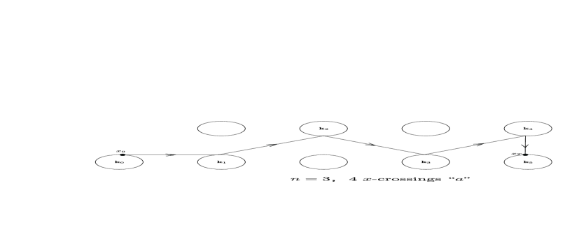
Figure 3.

Remark 2.19.

An admissible orbit segment $S^{[0,T]}x$ (described in the lemma above) will be called an “$a^{n+1}$-passage” with the connectors $\mathbf{l}_{0}$ and $\mathbf{l}_{n+1}$, where the first connector is called the “initial connector”, while the latter one is called the “terminal connector”. Observe that in this $a^{n+1}$-passage $S^{[0,T]}x$ the $x$-crossings “$a$” are in a natural, one-to-one correspondence with the reflections at the boundaries of $\mathcal{O}_{\mathbf{k}_{1}},\dots,\mathcal{O}_{\mathbf{k}_{n+1}}$, respectively. These reflections will be called the “eigenreflections” of the $a^{n+1}$-passage $S^{[0,T]}x$. The two reflections at the boundaries of $\mathcal{O}_{\mathbf{k}_{0}}$ and $\mathcal{O}_{\mathbf{k}_{n+2}}$ will not be considered as eigenreflections of this $a^{n+1}$-passage: The first one of them will actually be the last eigenreflection of a $b^{m}$-passage ($m\neq 0$) directly preceding the considered $a^{n+1}$-passage, while the second one will be the first eigenreflection of the $b^{p}$-passage ($p\neq 0$) directly following the $a^{n+1}$-passage $S^{[0,T]}x$. The shared passage vectors $\mathbf{l}_{0}$ and $\mathbf{l}_{n+1}$ will serve as connectors between the neighboring $a$- and $b$-passages. All passage vectors $\mathbf{l}_{i}$, used in this construction, have length $1$ or $\sqrt{2}$. We will say that the sequence of passage vectors $\sigma=(\mathbf{l}_{0},\mathbf{l}_{1},\dots,\mathbf{l}_{n+1})$ is the symbolic code of the considered $a^{n+1}$-passage $S^{[0,T]}x$.

Remark 2.20.

Clearly, similar statements are true on $a^{m}$-passages ($m<0$) and $b^{m}$-passages ($m\neq 0$). Also, in its current form of the lemma on $a^{n+1}$-passages, the first non-connector passage vector $\mathbf{l}_{1}=(1,1)$ could have been $(1,-1)$, by appropriately reflecting all other passage vectors about the $x$-axis.

Remark 2.21.

A few words are due here about the possible “exceptional” $b$ or $b^{-1}$ crossings of the initial and/or terminal connectors, mentioned at the end of the claim of the lemma: If the initial connector $\mathbf{l}_{0}=(1,0)$ happens to make an “exceptional” $y$-crossing $b$, then this crossing will be counted as the last $y$-crossing of the $b^{m}$-passage ($m>0$) preceding the considered $a^{n+1}$-passage. Similar statement can be said (mutatis mutandis) about a possible “exceptional” $y$-crossing ($b$ or $b^{-1}$) of the terminal connector $\mathbf{l}_{n+1}=(1,0)$.

Remark 2.22.

If $n>0$, then there are exactly $8$ different combinatorial possibilities for the symbolic code $\sigma=(\mathbf{l}_{0},\mathbf{l}_{1},\dots,\mathbf{l}_{n+1})$ of an $a^{n+1}$-passage: The $x$ coordinates of the connectors $\mathbf{l}_{0}$ and $\mathbf{l}_{n+1}$ can be $0$ or $1$ independently, whereas $\mathbf{l}_{1}$ can be $(1,1)$ or $(1,-1)$, also independently chosen from $\mathbf{l}_{0}$ and $\mathbf{l}_{n+1}$. However, for $n=0$ there are only $6$ possibilities for $\sigma=(\mathbf{l}_{0},\mathbf{l}_{1})$:

1. $\mathbf{l}_{0}=(0,1)$, $\mathbf{l}_{1}=(0,-1)$;

2. $\mathbf{l}_{0}=(0,-1)$, $\mathbf{l}_{1}=(0,1)$;

3. $\mathbf{l}_{0}=(1,0)$, $\mathbf{l}_{1}=(0,1)$;

4. $\mathbf{l}_{0}=(1,0)$, $\mathbf{l}_{1}=(0,-1)$;

5. $\mathbf{l}_{0}=(0,1)$, $\mathbf{l}_{1}=(1,0)$;

6. $\mathbf{l}_{0}=(0,-1)$, $\mathbf{l}_{1}=(1,0)$.

Consider an arbitrary element $w_{\infty}=\prod_{i=1}^{\infty}a^{n_{i}}b^{m_{i}}$ (an infinite word) of the set $\rm{Ends}(F_{2})$. For any natural number $N$ we want to construct a finite, admissible orbit segment $S^{[0,T_{N}]}x_{N}=x^{(N)}$, the associated word $w(x^{(N)})$ of which is $\prod_{i=1}^{N}a^{n_{i}}b^{m_{i}}:=w_{N}$, such that

$$\limsup_{N\to\infty}\frac{||w_{N}||}{T_{N}}\geq\frac{\sqrt{2}}{2}.$$

By symmetry, we may assume that the considered word $w_{\infty}$ begins with a power of “$a$” (as the notations above indicate), and that $n_{1}>0$. We shall use Lemma 2.18 by successively concatenating the $a^{n_{i}}$- and $b^{m_{i}}$-passages ($i=1,\dots,N$) to obtain the admissible orbit segment $x^{(N)}=S^{[0,T_{N}]}x_{N}$ with the associated word

$$w(x^{(N)})=w_{N}=\prod_{i=1}^{N}a^{n_{i}}b^{m_{i}}.$$

This will be achieved by constructing first the symbolic, admissible itinerary of $x^{(N)}$ containing only passage vectors $\mathbf{l}_{j}=\mathbf{k}_{j+1}-\mathbf{k}_{j}\in\mathbb{Z}^{2}$ of length $1$ and $\sqrt{2}$.

For simplicity (and by symmetry) we assume that $n_{1}>0$. First we construct the symbolic itinerary $(\mathbf{l}_{0},\dots,\mathbf{l}_{n_{1}})$ of an $a^{n_{1}}$-passage by taking $\mathbf{l}_{0}=(1,0)$, $\mathbf{l}_{j}=(1,\,(-1)^{j+1})$ for $j=1,2,\dots,n_{1}-1$. The terminal connector $\mathbf{l}_{n_{1}}$ will be carefully chosen, depending on the parity of $n_{1}$ and the sign of the integer $m_{1}$. By symmetry we may assume that $\mathbf{l}_{n_{1}-1}=(1,\,-1)$, i. e. that $n_{1}$ is an odd number. In the construction of the terminal connector $\mathbf{l}_{n_{1}}$ and the symbolic itinerary $(\mathbf{l}_{n_{1}},\mathbf{l}_{n_{1}+1},\dots,\mathbf{l}_{n_{1}+|m_{1}|})$ of the subsequent $b^{m_{1}}$-passage we will distinguish between two, essentially different cases.

Case I. $m_{1}>0$

In this case we take $\mathbf{l}_{n_{1}}=(0,1)$ and, furthermore, $\mathbf{l}_{j}=((-1)^{j},\,1)$ for $j=n_{1}+1,n_{1}+2,\dots,n_{1}+|m_{1}|-1$. The terminal connector $\mathbf{l}_{n_{1}+|m_{1}|}$ of this $b^{m_{1}}$-passage will be carefully chosen by a coupling process (similar to the one that we are just describing here) to couple the $b^{m_{1}}$-passage with the subsequent $a^{n_{2}}$-passage.

Case II. $m_{1}<0$

In this case we take $\mathbf{l}_{n_{1}}=(1,0)$, $\mathbf{l}_{j}=((-1)^{j+1},\,-1)$ for $j=n_{1}+1,n_{1}+2,\dots,n_{1}+|m_{1}|-1$. Again, the terminal connector $\mathbf{l}_{n_{1}+|m_{1}|}$ of this $b^{m_{1}}$-passage will be carefully chosen by a coupling process to couple the $b^{m_{1}}$-passage with the subsequent $a^{n_{2}}$-passage.

It is clear that the above process can be continued (by changing whatever needs to be changed, according to the apparent mirror symmetries of the system) to couple together the subsequent $a^{n_{1}}$-, $b^{m_{1}}$-, $a^{n_{2}}$-, $b^{m_{2}}$-,$\dots$, $a^{n_{N}}$-, and $b^{m_{N}}$-passages. In this way we obtain the admissible symbolic itinerary $(\mathbf{l}_{0},\mathbf{l}_{1},\dots,\mathbf{l}_{||w_{N}||})$ of a potential admissible orbit segment $x^{(N)}$ with the associated word

$$w(x^{(N)})=w_{N}=\prod_{i=1}^{N}a^{n_{i}}b^{m_{i}}.$$

The existence of such an admissible orbit segment $x^{(N)}$ is guaranteed by Theorem 2.2 of [BMS06], using an orbit length minimizing principle in the construction. This means that a required orbit segment $x^{(N)}$ can be obtained by minimizing the length of all piecewise linear curves (broken lines) $P_{0}P_{1}\dots P_{L+1}$ ($L=||w_{N}||=\sum_{i=1}^{N}(|n_{i}|+|m_{i}|)$) for which the corner points $P_{j}$ belong to the obstacle (the closed disk) $\mathcal{O}_{\mathbf{k}_{j}}$ ($j=0,1,\dots,L+1$) with $\mathbf{k}_{j}=\sum_{i=0}^{j-1}\mathbf{l}_{i}$. Clearly, the length $T_{N}$ of the arising orbit segment $x^{(N)}$ is less than the length of the broken line connecting the consecutive centers $\mathbf{k}_{j}$ ($0\leq j\leq L+1$) of the affected obstacles, and this latter number is $\sum_{j=0}^{L}||\mathbf{l}_{j}||\leq\sqrt{2}(L+1)$. Thus, we get that

$$\frac{||w_{N}||}{T_{N}}>\frac{L}{\sqrt{2}(L+1)},$$

and this proves Theorem 2.16.

We note that if a point $(t,e)$ turns out to be a limiting point of a sequence of admissible orbit segments with passage vectors of length $1$ or $\sqrt{2}$, then any other point $(t_{1},e)\in C$ with $0\leq t_{1}\leq t$ is also such a limiting point. Indeed, by inserting the necessary amount of “idle sequences” $\alpha\alpha^{-1}\alpha\alpha^{-1}\cdots$ in the itinerary, we can decrease the ratios $\|w(\sigma)\|/T(\sigma)$ (and their limits) as we wish. This finishes the proof of the theorem. ∎

An immediate consequence of the last argument is

Corollary 2.23.

The set $AR$ is star-shaped from the view point $(0,0)\in C$, i.e., $(t,e)\in AR$ and $0\leq t_{1}\leq t$ imply that $(t_{1},e)\in AR$.

The concluding result of this section shows that the lower estimate $\sqrt{2}/2$ for the radial size of $AR$ is actually sharp, at least in some directions $w_{\infty}\in\rm{Ends}(\textbf{F}_{2})$ and in the small obstacle limit $r_{0}\to 0$.

Proposition 2.24.

Consider the direction

$$w_{\infty}=aba^{-1}b^{-1}aba^{-1}b^{-1}\dots\in\rm{Ends}(\textbf{F}_{2}),$$

i. e. the “infinite power” of the commutator element $[a,b]=aba^{-1}b^{-1}$. We claim that the radial size

$$\sigma=\sigma(r_{0},w_{\infty})=\sup\left\{t\in\mathbb{R}_{+}\big{|}\;(t,\,w_{\infty})\in R\right\}$$

of the full rotation set $R$ in the direction of $w_{\infty}$ has the limiting value $\sqrt{2}/2$, as $r_{0}\to 0$. In particular, similar statement holds true for the radial size of the smaller, admissible rotation set $AR$ in the same direction. Thus, the lower estimate $\sqrt{2}/2$ for the radial size of $AR$ (of $R$) in this direction cannot be improved in the small obstacle limit $r_{0}\to 0$. We recall that, according to Theorem 2.16 above, $\sigma(r_{0},e)\geq\sqrt{2}/2$ for all $r_{0}$ and all $e\in\rm{Ends}(\textbf{F}_{2})$.

Proof.

Consider an infinite sequence $(x_{n})_{n=1}^{\infty}$ of orbit segments

$$x_{n}=\left\{x_{n}(t)\big{|}\;0\leq t\leq T_{n}\right\}$$

with $T_{n}\nearrow\infty$, $w(x_{n})=(aba^{-1}b^{-1})^{k_{n}}$, $k_{n}\nearrow\infty$, and

$$\lim_{n\to\infty}\frac{4k_{n}}{T_{n}}=\sigma(r_{0},\,w_{\infty}).$$

We may assume that the relevant $x$-crossings “$a$” of $x_{n}$ (relevant in the sense that their symbol $a$ remains in the associated word $w(x_{n})$ after all possible shortenings) take place between the obstacles at $(0,0)$ and $(0,-1)$, the relevant $y$-crossings “$b$” occur between the obstacles at $(0,0)$ and $(1,0)$, the relevant $x$-crossings “$a^{-1}$” happen between the obstacles at $(0,0)$ and $(0,1)$ and, finally, the relevant $y$-crossings “$b^{-1}$” take place between the obstacles at $(0,0)$ and $(-1,0)$, i. e. $x_{n}$ circles around the central obstacle $\mathcal{O}_{(0,0)}$ counterclockwise. The proof of the inequality

$$\limsup_{r_{0}\to 0}\sigma(r_{0},\,w_{\infty})\leq\frac{\sqrt{2}}{2}$$

will be based on the following, elementary geometric observation:

Lemma 2.25.

Let $N$ be a natural number and

$$\Gamma=\left\{\gamma(t)\big{|}\;0\leq t\leq T\right\}$$

be a piecewise linear curve (a broken line) in $\operatorname{\mathbb{R}}^{2}$ parametrized with the arc length, enjoying the following properties:

1. every vertex (corner) of $\Gamma$ is an integer point;

2. $(0,0)\not\in\Gamma$;

3. $\Gamma$ winds around the origin at least $N$ times, i. e.

   $$\int_{0}^{T}\dot{\omega}(t)dt\geq 2\pi N,$$

   where $\omega(t)$ is the angular polar coordinate of $\gamma(t)$.

We claim that $T\geq 4\sqrt{2}N$, and the equation holds if and only if $\Gamma$ connects the lattice points $(1,0)$, $(0,1)$, $(-1,0)$, and $(0,-1)$ in this cyclic order.

Since the proof of this result is a simple, elementary geometric argument (though with a little bit tedious investigation of a few cases), we omit it, and immediately turn to the proof of the proposition.

For $n=1,2,\dots$ we define a broken line $\Gamma_{n}$, fulfilling all conditions of the previous lemma with $N=k_{n}$, by

1. considering all centers $c_{1},c_{2},\dots,c_{m}$ ($c_{i}\in\mathbb{Z}^{2}$) of the obstacles visited by $x_{n}$ in the time order $x_{n}$ visits them;

2. dropping the possible appearances of the origin from the above sequence $c_{1},c_{2},\dots,c_{m}$;

3. constructing $\Gamma_{n}$ by connecting the lattice points $c_{1},c_{2},\dots,c_{m}$ (in this order) and, by adding a bounded extension to $\Gamma_{n}$ if necessary, ensuring that $\Gamma_{n}$ winds around the origin at least $k_{n}$ times.

Observe that the length $|AB|$ of any billiard orbit segment, connecting two consecutive collisions, is always between $d-2r_{0}$ and $d$, where $d$ is the distance between the centers of the obstacles affected by the collisions. Therefore, by the previous lemma we get the following inequality for the length $T_{n}$ of $x_{n}$:

$$\frac{T_{n}}{1-2r_{0}}+C\geq 4\sqrt{2}k_{n}$$

with some constant $C>0$. This inequality implies

$$\sigma(r_{0},\,w_{\infty})=\lim_{n\to\infty}\frac{4k_{n}}{T_{n}}\leq\frac{\sqrt{2}}{2(1-2r_{0})},$$

thus

$$\limsup_{r_{0}\to 0}\sigma(r_{0},w_{\infty})\leq\frac{\sqrt{2}}{2},$$

as claimed by the proposition. ∎

3. Corollaries and Concluding Remarks

The first corollary listed in this section is a byproduct of the proof of Theorem 2.12. It provides a positive constant as the upper estimate for the topological entropy $h_{\text{top}}(r_{0})$ of our considered $2D$ billiard flow with one obstacle.

Theorem 3.1.

For the topological entropy $h_{\text{top}}(r_{0})$ of the billiard flow studied in this paper we have the following upper estimate

$$h_{\text{top}}(r_{0})\leq 6\sqrt{2}\ln 2=5.8815488\dots$$

Remark 3.2.

The above corollary should be compared to (and explained in the framework of) some earlier results by Burago-Ferleger-Kononenko. In [BFK98], the authors also enumerate all possible homotopical-combinatorial types of trajectories, and they prove the existence of a limit

$$0<\lim_{r_{0}\rightarrow 0}h_{\text{top}}(r_{0})=c_{0}<\infty.$$

along with the lower estimate $\ln 3\leq c_{0}$ and an implicit upper bound in terms of the similar entropy limit for the $3D$ Lorentz gas. In Theorem 3.1 we obtained a concrete upper bound for $c_{0}$.

Proof of 3.1..

We subdivide the periodic billiard table $\mathcal{Q}$ (the configuration space) into five pairwise disjoint domains $\mathcal{D}_{1},\mathcal{D}_{2}^{\pm},\mathcal{D}_{3}^{\pm}$ with piecewise linear boundaries as depicted in the figure below. The domains $\mathcal{D}_{k}^{+}$ ($k=2,3$) consist of all points $(x_{1},x_{2})\in\mathcal{Q}$ for which the fractional part $\{x_{k-1}\}$ of $x_{k-1}$ satisfies the inequality $\{x_{k-1}\}\leq\varepsilon_{0}$ (for some fixed, small $\varepsilon_{0}>0$), the domains $\mathcal{D}_{k}^{-}$ ($k=2,3$) consist of all points $(x_{1},x_{2})\in\mathcal{Q}$ for which $\{x_{k-1}\}\geq 1-\varepsilon_{0}$, while $\mathcal{D}_{1}$ is the closure $\overline{\mathcal{Q}\setminus(\mathcal{D}_{2}^{-}\cup\mathcal{D}_{2}^{+}\cup\mathcal{D}_{3}^{-}\cup\mathcal{D}_{3}^{+})}$ of the set $\mathcal{Q}\setminus(\mathcal{D}_{2}^{-}\cup\mathcal{D}_{2}^{+}\cup\mathcal{D}_{3}^{-}\cup\mathcal{D}_{3}^{+})$.

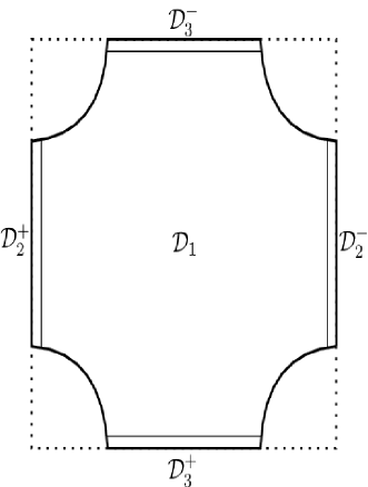
Figure 4.

The union $\mathcal{Q}=\mathcal{D}_{1}\cup\mathcal{D}_{2}^{-}\cup\mathcal{D}_{2}^{+}\cup\mathcal{D}_{3}^{-}\cup\mathcal{D}_{3}^{+}$ is an almost disjoint one: these domains only intersect at their piecewise linear boundaries. Thus, from the dynamical viewpoint $\mathcal{Q}=\mathcal{D}_{1}\cup\mathcal{D}_{2}^{-}\cup\mathcal{D}_{2}^{+}\cup\mathcal{D}_{3}^{-}\cup\mathcal{D}_{3}^{+}$ is a partition $\Pi$.

We claim that $\Pi$ is a generating partition, meaning that the supremum (the coarsest common refinement) $\bigwedge_{n=-\infty}^{\infty}S^{-n\epsilon_{0}}(\Pi)$ of the partitions $S^{-n\epsilon_{0}}(\Pi)$ is the trivial partition into the singletons, modulo the zeroe-measured sets. Indeed, if two phase points $x=(q_{1},v_{1})$ and $y=(q_{2},v_{2})$ ($q_{1},q_{2}\in\mathcal{Q}$, $v_{i}\in\operatorname{\mathbb{R}}^{2}$, $\|v_{i}\|=1$) share the same symbolic future itineraries (recorded at $n\epsilon_{0}$ moments of time) with respect to the partition $\Pi$, then, as an elementary inspection shows, $S^{\tau}y$ and $x$ belong to the same local stable curve, where $\tau\in\operatorname{\mathbb{R}}$ is a time-synchronizing constant. Similar results apply to the shared symbolic itineraries in the past and the unstable curves. These facts imply that $x=S^{\tau}y$ (with some $\tau\in\operatorname{\mathbb{R}}$), whenever $x$ and $y$ share identical $\Pi$-itineraries in both time directions, i.e. $x=y$ for a typical pair $(x,y)$, so $\Pi$ is a generating partition.

For any time $T>0$ ($T$ will eventually go to infinity) denote by $N(T)$ the number of all possible $\Pi$-itineraries of trajectory segments $S^{[0,T]}x$, $x\in\mathcal{M}$. It follows from the generating property of $\Pi$ that

(3.3) $$h_{\text{top}}=\lim_{T\rightarrow\infty}\frac{1}{T}\ln N(T).$$

It is clear that any orbit segment $\left\{x(t)|0\leq t\leq T\right\}$ alternates between the domains $\mathcal{D}_{1}$ and $\mathcal{D}^{*}=\overline{\mathcal{Q}\setminus\mathcal{D}_{1}}$. Consider an orbit segment $x=\left\{x(t)\big{|}\;0\leq t\leq T\right\}$ lifted to the covering space $\tilde{\mathcal{Q}}$ of $\mathcal{Q}$. Let $\tau_{1}$ be a time when $x$ leaves the domain $D_{2}^{+}$ ($D_{2}^{-}$), and $\tau_{2}$ be the time when $x$ re-enters the same domain $D_{2}^{+}$ ($D_{2}^{-}$) the next time, $0\leq\tau_{1}<\tau_{2}\leq T$. The proof of the lemma following Theorem 2.12 shows that

$$\int_{\tau_{1}}^{\tau_{2}}\left|\dot{x}_{1}(t)\right|dt\geq 1-\varepsilon_{0}.$$

Therefore, the number of times the orbit segment $x$ visits the domain $D_{2}^{+}$ ($D_{2}^{-}$) is at most

$$\frac{1}{1-\varepsilon_{0}}\cdot\int_{0}^{T}\left|\dot{x}_{1}(t)\right|dt+1.$$

Applying this upper estimate to $D_{2}^{+}$ and $D_{2}^{-}$, then the analogous upper estimates for the number of visits to $D_{3}^{\pm}$, and, finally, taking the sum of the arising four estimates, we get that the total number of visits by $x$ to the four domains $D_{2}^{\pm}$, $D_{3}^{\pm}$ is at most

$$\frac{2}{1-\varepsilon_{0}}\cdot\int_{0}^{T}\left(\left|\dot{x}_{1}(t)\right|+\left|\dot{x}_{2}(t)\right|\right)dt+4\leq\frac{2\sqrt{2}T}{1-\varepsilon_{0}}+4.$$

Since $x$ alternates between $D_{1}$ and the union of the other four domains, the total number of times $x$ visits $D_{1}$ is at most

$$f(T,\,\varepsilon_{0}):=\frac{2\sqrt{2}T}{1-\varepsilon_{0}}+5.$$

After entering any of the domains $\mathcal{D}_{2}^{\pm}$, $\mathcal{D}_{3}^{\pm}$, the orbit segment $\sigma$ has two sides of this domain (i. e. two combinatorial possibilities) to exit it, whereas, after entering the domain $\mathcal{D}_{1}$, it has four sides of $\mathcal{D}_{1}$ to leave it. This argument immediately yields the upper estimate

(3.4) $$N(T)\leq 8^{f(T,\,\varepsilon_{0})}$$

for the number $N(T)$ of all possible symbolic types of orbit segments of length $T$. In light of (3.3), the above inequality proves the upper estimate of Theorem 3.1, once we take the natural logarithm of (3.4), take the limit as $T\to\infty$, and, finally, the limit as $\varepsilon_{0}\to 0$. ∎

Corollary 3.5 (Corollary of Theorem 2.16).

For the topological entropy $h_{\text{top}}(r_{0})$ of the billiard flow (with one circular obstacle of radius $r_{0}$ inside $\mathbb{T}^{2}$) we have the lower estimate

$$h_{\text{top}}(r_{0})\geq\frac{\ln 3}{\sqrt{2}}\approx 0.776836199\dots$$

Proof. (A sketch.) Theorem 2.16 says that the words $w\left(\left\{x(t)|\;0\leq t\leq T\right\}\right)$ corresponding to all orbits $\left\{x(t)|\;0\leq t\leq T\right\}$ of length $T$ fill in the ball of radius $T/\sqrt{2}$ in the Cayley graph of the group $F_{2}$. Hence the number of different homotopy types of these orbits $\left\{x(t)|\;0\leq t\leq T\right\}$ is at least $\text{const}\cdot 3^{T/\sqrt{2}}$. Take the natural logarithm of this lower estimate, divide by $T$, and pass to the limit as $T\to\infty$ to get the claim of the corollary. ∎

Let $x_{T_{0}}=\left\{x(t)|\;0\leq t\leq T_{0}\right\}$ be a periodic orbit with period $T_{0}$, and $w_{0}=w\left(x_{T_{0}}\right)\in F_{2}(a,b)$ the symbolic word corresponding to it. Finally, let $w_{\infty}=w_{0}w_{0}w_{0}\dots\in\text{Ends}(F_{2})$ be the infinite power of $w_{0}$. It is clear that the homotopical rotation number $(t,\,e)=(t,\,w_{\infty})\in C$ of the full (periodic) orbit $x$ exists, i. e.

$$t=\lim_{T\to\infty}\frac{\left\|w\left(\left\{x(t)|\;0\leq t\leq T\right\}\right)\right\|}{T}=\frac{||w_{0}||}{T_{0}},$$

$$e=w_{\infty}=\lim_{T\to\infty}w\left(\left\{x(t)|\;0\leq t\leq T\right\}\right).$$

Note that $t=0$ if and only if $w_{0}=1$. In this case the directional component $e=w_{\infty}\in\text{Ends}(F_{2})$ of the rotation number is undefined.

Remark 3.6.

We observe that in Definition 2.8 of the admissible homotopical rotation set $AR\subset C$ we can select the approximating orbit segments $x_{i}=\{x_{i}(\tau)|0\leq\tau\leq T_{i}\}$ to be periodic with period $T_{i}$ (see Theorem 2.2 of [BMS06]). Thus, the homotopical rotation numbers $(t,e)\in C$

$$e=\lim_{T\rightarrow\infty}w(\{x(\tau)|0\leq\tau\leq T\})\in\text{Ends}(F_{2}),$$

$$t=\lim_{T\rightarrow\infty}\frac{\|w(\{x(\tau)|0\leq\tau\leq T\})\|}{T},$$

corresponding to admissible periodic orbits $\{x(\tau)|\tau\in\operatorname{\mathbb{R}}\}$ form a dense subset in $AR$.

Remark 3.7.

The problem of defining and thoroughly studying the analogous homotopical rotation numbers in the case of $N$ round obstacles in $\mathbb{T}^{2}$ $(N\geq 2)$ is much more complex than the case $N=1$. Indeed, the fundamental group $G=\pi_{1}(\mathcal{Q})$ turns out to be the group $\textbf{F}_{N+1}$ freely generated by $N+1$ elements $a_{1},a_{2},\ldots,a_{N+1}$ (see [Mas91]). The complexity of the problem is partially explained by the following fact: the “abelianized” version $G/G^{\prime}$ (where $G^{\prime}=[G,G]$ is the commutator subgroup of $G$) is isomorphic to $\operatorname{\mathbb{Z}}^{N+1}$. In the case $N=1$ the group $\operatorname{\mathbb{Z}}^{N+1}=\operatorname{\mathbb{Z}}^{2}$ coincides with the lattice group of periodicity of the billiard system, and this coincidence establishes a strong connection between the newly introduced homotopical (non-commutative) rotation number $(t,e)\in C$ of a trajectory $\{x(\tau)|\tau\in\operatorname{\mathbb{R}}\}$,

$$e=\lim_{T\rightarrow\infty}w(\{x(\tau)|0\leq\tau\leq T\})=\lim_{T\rightarrow\infty}w_{T}$$

$$t=\lim_{T\rightarrow\infty}\frac{\|w(\{x(\tau)|0\leq\tau\leq T\})\|}{T}=\lim_{T\rightarrow\infty}\frac{\|w_{T}\|}{T}$$

and the traditional (commutative) rotation vector $\rho$ of the same trajectory as follows:

$$\rho=\lim_{T\rightarrow\infty}\frac{1}{T}\pi(w_{T})\in\operatorname{\mathbb{R}}^{2},$$

where $\pi:G\rightarrow G/G^{\prime}=\operatorname{\mathbb{Z}}^{2}$ is the natural projection. Clearly, there is no such straightforward correspondence between the two types of rotation numbers (vectors) in the case $N\geq 2$.

Remark 3.8.

If one carefully studies all the proofs and arguments of this paper, it becomes obvious that the round shape of the sole obstacle $\mathcal{O}$ was essentially not used. Thus, all the above results carry over to any other billiard table model on $\mathbb{T}^{2}$ with a single strictly convex obstacle with smooth boundary $\partial\mathcal{O}$, provided that $\mathcal{O}$ is small in the sense of [BMS06], i.e., $\mathcal{O}$ is contained in a disk of radius $r_{0}$, $r_{0}<\sqrt{2}/4$. (And $r_{0}<\sqrt{5}/10$ for Theorem 2.16.)

Remark 3.9.

One can ask similar questions (regarding the noncommutative rotation numbers/sets) for toroidal billiards in the configuration space $\mathcal{Q}$, where

$$\mathcal{Q}=\mathbb{T}^{d}\setminus\bigcup_{i=1}^{N}\mathcal{O}_{i},$$

with $d\geq 3$ and $N$ mutually disjoint, compact, strictly convex obstacles $\mathcal{O}_{i}$ with smooth boundaries. Such a space $\mathcal{Q}$ is, obviously, homotopically equivalent to the $d$-torus $\mathbb{T}^{d}$ with $N$ points removed from it (a “punctured torus”); however, due to the assumption $d\geq 3$, the fundamental group $\pi_{1}(\mathcal{Q})$ of such a space is naturally isomorphic to $\pi_{1}(\mathbb{T}^{d})\cong\operatorname{\mathbb{Z}}^{d}$, for the homotopical deformations of loops can always avoid the removed $N$ points. Thus, for such a system the homotopical rotation numbers and sets coincide with the usual commutative notions, studied in [BMS06].

References

- [BFK98] D. Burago, S. Ferleger, and A. Kononenko, Topological entropy of semi-dispersing billiards, Ergod. Th. & Dynam. Sys. 18 (1998), 791–805.
- [BMS06] A. Blokh, M. Misiurewicz, and N. Simányi, Rotation sets of billiards with one obstacle, Commun. Math. Phys. 266 (2006), 239–265.
- [Boy00] P. Boyland, New dynamical invariants on hyperbolic manifolds, Israel J. Math. 119 (2000), 253–289.
- [CP93] M. Coornaert and A. Papadopoulos, Symbolic dynamics and hyperbolic groups, Springer-Verlag, New York, 1993.
- [Eng89] R. Engelking, General topology revised and completed edition, Heldermann, Berlin, 1989.
- [Mas91] W. S. Massey, A basic course in algebraic topology, Springer-Verlag, New York, 1991.
- [Mor24] M. Morse, A fundamental class of geodesics on any closed surface of genus greater than one, Trans. Amer. Math. Soc. 26 (1924), 25–60.
- [Sch57] S. Schwartzman, Asymptotic cycles, Annals of Math. 66 (1957), 270–284.