GODDeS: Globally $\epsilon$-Optimal Routing Via Distributed Decision-theoretic Self-organization

Abstract

This paper introduces GODDeS: a fully distributed self-organizing decision-theoretic routing algorithm designed to effectively exploit high quality paths in lossy ad-hoc wireless environments, typically with a large number of nodes. The routing problem is modeled as an optimal control problem for a decentralized Markov Decision Process, with links characterized by locally known packet drop probabilities that either remain constant on average or change slowly. The equivalence of this optimization problem to that of performance maximization of an explicitly constructed probabilistic automata allows us to effectively apply the theory of quantitative measures of probabilistic regular languages, and design a distributed highly efficient solution approach that attempts to minimize source-to-sink drop probabilities across the network. Theoretical results provide rigorous guarantees on global performance, showing that the algorithm achieves near-global optimality, in polynomial time. It is also argued that GODDeS is significantly congestion-aware, and exploits multi-path routes optimally. Theoretical development is supported by high-fidelity network simulations.

I Introduction & Motivation

The routing problem has been widely studied in the context of ad-hoc wireless networks, and reported algorithms can be broadly classified as follows. A routing protocol is pro-active (DBF ($e.g.$ Distributed Bellman-Ford) [1] and DSDV (Highly Dynamic Destination-Sequenced Distance Vector routing) [2]), if fresh destination lists and their routes are maintained by periodically distributing routing tables; it is reactive ($e.g.$ AODV (Ad-hoc On-demand Distance Vector) [3] and DSR (Dynamic Source Routing) [4]) if routes are computed if and when necessary by flooding the network with Route Request packets. Pro-active protocols suffer from expensive route maintenance and slow reaction to topology changes, while reactive methods have high latency in discovery and induce congestion due to periodic flooding. Hybrid protocols attempt to combine advantages of both philosophies $e.g.$ HRPLS (Hybrid Routing Protocol for Large Scale Mobile Ad Hoc Networks with Mobile Backbones) [5] and HSLS (Hazy Sighted Link State routing protocol) [6]. Protocols may also be classified as being either distance-vector or link-state driven. In the former case, the computed distance to all nodes is is exchanged with neighbors ($e.g.$ DSDV, AODV); while in the latter computed distances to the neighbors is exchanged with all nodes ($e.g.$ OLSR (Optimized Link State Routing) [7], ZHLS (Zone-Based Hierarchical Link State) [8]). Link state protocols maintain better Quality Of Service (QOS), but suffer from poor scalability. Distance vector protocols have less control traffic, but maintaining QOS is more difficult. Other approaches use geographic, or power information, and in the context of sensor networks, query based routing strategies ($e.g.$ Directed Diffusion [9]) have been proposed.

Reported ad hoc routing protocols for wireless networks primarily focus on node mobility, rapidly changing topologies, overhead, and scalability; with little attention paid to finding high-quality paths in the face of lossy wireless links. An implicit assumption is that links either work well or don’t work at all; which is not reasonable in the wireless case where many links have intermediate loss ratios. This problem has been partially addressed by designing new quality-aware metrics such as the expected transmission count (ETX) [10], where the authors correctly note “minimizing hop-count maximizes the distance traveled by each hop, which is likely to minimize signal strength and maximize the loss ratio”. Even if the best route is one with minimal hop-count, there may be many routes (particularly in dense networks) of the same minimum length with widely varying qualities; arbitrary choice made by most minimum hop-count metrics is not likely to select the best. The problem is also crucial in multi-rate networks [11], where the routing protocol must select from the set of available links. While in single-rate networks all links are equivalent, in multi-rate networks each available link may operate at a different rate. Thus the routing protocol is presented with a complex trade-off decision: Long distance links take fewer hops, but the links operate slower; short links can operate at high rates, but more hops are required.

In this paper, we give a theoretical solution to this potentially large-scale decision problem via formulating a probabilistic routing policy that very nearly minimizes the end-to-end packet drop probabilities. In particular, the routing problem is modeled and solved as an optimal control problem for a Decentralized Markov Decision Process (D-MDP). Extensively used for centralized decision making in stochastic environments, Markov decision processes (MDPs) have been recently, extended to decentralized multi-agent settings [12]. In the context of ad-hoc routing, we begin by assuming that the communication links are imperfect, and are being characterized by locally known drop probabilities. The mean or expected values of the link-specific drop probabilities, and the network topology is assumed to be are either constant or changing over a time scale which is significantly slower compared to that of the communication dynamics. We then seek local routing decisions that maximize throughput in the sense of minimizing the source-to-sink probability of packet-drops. The Markov structure emerges, since we assume that the local link-specific drop probabilities are independent of the history of sequential link traversal by individual packets.

The results developed in this paper effectively resolve the issues described above (and does more, actually attaining near global optimality); and would seem to be a straightforward solution scheme. Nevertheless, to the best of the author’s knowledge, such an approach has not been previously investigated. The reason for this apparent neglect (which also highlights the key theoretical contribution of this paper) is as follows: Recent investigations [12, 13] into the solution complexity of decentralized Markov decision processes have shown that the problem is exceptionally hard even for two agents; illustrating a fundamental divide between centralized and decentralized control of MDP. In contrast to the centralized approach, the decentralized case provably does not admit polynomial-time algorithms. Furthermore, assuming $\textrm{EXP}=\textrm{NEXP}$, the problems require super-exponential time to solve in the worst case. Such negative results do not preclude the possibility of obtaining near-optimal solutions efficiently. This is precisely what we achieve in this paper, in the context of the routing problem. We show that a highly efficient, fully distributed, decision algorithm can be designed that effectively solves the distributed MDP such that the control policy, on convergence, is within an $\epsilon$ bound of the global optimal. Furthermore, one can freely choose the error bound $\epsilon$ (and make it as small as one wishes), with the caveat that the convergence time increases (with no finite upper bound) with decreasing $\epsilon$.

We call this algorithm GODDeS (Globally $\epsilon$-Optimal Routing Via Distributed Decision-theoretic Self-organization). Instead of using a standard MDP formulation, we use a problem representation based on Probabilistic Finite State Automata (PFSA), which allows us to set up the decision problem as that of performance maximization of PFSA, and obtain solutions using the recently reported quantitative measures of probabilistic regular languages [14]. This shift of modeling paradigm is the quintessential insight that allows one to achieve near-global optimality in polynomial time. Theoretical results also establish that GODDeS is highly scalable, optimally take advantage of existing multi-path routes, and is expected to be significantly congestion-aware. For simplicity of exposition, a single sink is considered throughout the paper. This is not a serious restriction, since the results carry over to the general case with ease. The resulting algorithm is both pro-active and reactive, but not in the usual sense of reported hybrid protocols. It uses both distance-vector (in a generalized sense via the language-measure construction) and link-state information, and uses local multi-cast to forward messages; optimally taking advantage of multi-path routing.

The rest of the paper is organized in six sections. Section II briefly summarizes the theory of quantitative measures of probabilistic regular languages, and the pertinent approaches to centralized performance maximization of PFSA. Section III develops the PFSA model of an ad-hoc network, and Section IV presents the key theoretical development for decentralized PFSA optimization. Section V validates the theoretical development with high fidelity simulation results on the NS2 network simulator, and discusses the key properties and characteristics for the proposed routing algorithm. The paper is summarized and concluded in Section VII with recommendations for future work.

II Background: Language Measure Theory

This section summarizes the concept of signed real measure of probabilistic regular languages, and its application in performance optimization of probabilistic finite state automata (PFSA) [14]. A string over an alphabet ($i.e.$ a non-empty finite set) $\Sigma$ is a finite-length sequence of symbols from $\Sigma$ [15]. The Kleene closure of $\Sigma$, denoted by $\Sigma^{*}$, is the set of all finite-length strings of symbols including the null string $\epsilon$. The string $xy$ is the concatenation of strings $x$ and $y$, and the null string $\epsilon$ is the identity element of the concatenative monoid.

Definition 1 (PFSA)

A PFSA $G$ over an alphabet $\Sigma$ is a sextuple $(Q,\Sigma,\delta,\widetilde{\Pi},\chi,\mathscr{C})$, where $Q$ is a set of states, $\delta:Q\times\Sigma^{\star}\rightarrow Q$ is the (possibly partial) transition map; $\widetilde{\Pi}:Q\times\Sigma\rightarrow[0,1]$ is an output mapping, known as the probability morph function that specifies the state-specific symbol generation probabilities and satisfies $\forall q_{i}\in Q,\sigma\in\Sigma,\widetilde{\Pi}(q_{i},\sigma)\geqq 0$, and $\sum_{\sigma\in\Sigma}\widetilde{\Pi}(q_{i},\sigma)=1$, the state characteristic function $\chi:Q\rightarrow[-1,1]$ assigns a signed real weight to each state, and $\mathscr{C}$ is the set of controllable transitions that can be disabled (Definition 2).

Definition 2 (Control Philosophy)

If $\delta(q_{i},\sigma)=q_{k}$, then the disabling of $\sigma$ at $q_{i}$ prevents the state transition from $q_{i}$ to $q_{k}$. Thus, disabling a transition $\sigma$ at a state $q$ replaces the original transition with a self-loop with identical occurrence probability, $i.e.$ we now have $\delta(q_{i},\sigma)=q_{i}$. Transitions that can be so disabled are controllable, and belong to the set $\mathscr{C}$.

Definition 3

The language $L(q_{i})$ generated by a PFSA $G$ initialized at the state $q_{i}\in Q$ is defined as: $L(q_{i})=\{s\in\Sigma^{*}\ |\ \delta(q_{i},s)\in Q\}$ Similarly, for every $q_{j}\in Q$, $L(q_{i},q_{j})$ denotes the set of all strings that, starting from the state $q_{i}$, terminate at the state $q_{j}$, i.e., $L(q_{i},q_{j})=\{s\in\Sigma^{*}\ |\ \delta(q_{i},s)=q_{j}\in Q\}$

Definition 4 (State Transition Matrix)

The state transition probability matrix $\Pi\in[0,1]^{\textrm{{Card}}(Q)\times\textrm{{Card}}(Q)}$, for a given PFSA is defined as: $\forall q_{i},q_{j}\in Q,\Pi_{ij}=\sum_{\sigma\in\Sigma\ \mathrm{s.t.}\ \delta(q_{i},\sigma)=q_{j}}\widetilde{\Pi}(\sigma,q_{i})$ Note that $\Pi$ is a square non-negative stochastic matrix [16], where $\Pi_{ij}$ is the probability of transitioning from $q_{i}$ to $q_{j}$.

Notation 1

We use matrix notations interchangeably for the morph function $\widetilde{\Pi}$. In particular, $\widetilde{\Pi}_{ij}=\widetilde{\Pi}(q_{i},\sigma_{j})$ with $q_{i}\in Q,\sigma_{j}\in\Sigma$. Note that $\widetilde{\Pi}\in[0,1]^{\textrm{{Card}}(Q)\times\textrm{{Card}}(\Sigma)}$ is not necessarily square, but each row sums up to unity.

A signed real measure [17] $\nu^{i}:{2^{L(q_{i})}}\rightarrow\mathbb{R}\equiv(-\infty,+\infty)$ is constructed on the $\sigma$-algebra $2^{L(q_{i})}$ [14], implying that every singleton string set $\{s\in L(q_{i})\}$ is a measurable set.

Definition 5 (Language Measure)

Let $\omega\in L(q_{i},q_{j})\subseteq 2^{L(q_{i})}$. The signed real measure $\nu^{i}_{\theta}$ of every singleton string set $\{\omega\}$ is defined as: $\nu^{i}_{\theta}(\{\omega\})\triangleq\theta(1-\theta)^{|\omega|}\widetilde{\Pi}(q_{i},\omega)\chi(q_{j})$. For every choice of the parameter $\theta\in(0,1)$, the signed real measure of a sublanguage $L(q_{i},q_{j})\subseteq L(q_{i})$ is defined as: $\nu^{i}_{\theta}(L(q_{i},q_{j}))\triangleq\sum_{\omega\in L(q_{i},q_{j})}\theta(1-\theta)^{|\omega|}\widetilde{\Pi}(q_{i},\omega)\chi_{j}$. Similarly, the measure of $L(q_{i})$, is defined as $\nu^{i}_{\theta}(L(q_{i}))\triangleq\sum_{q_{j}\in Q}\nu^{i}_{\theta}(L_{i,j})$.

Notation 2

For a given PFSA, we interpret the set of measures $\nu^{i}_{\theta}(L(q_{i}))$ as a real-valued vector of length $\textrm{{Card}}(Q)$ and denote $\nu^{i}_{\theta}(L(q_{i}))$ as $\nu_{\theta}|_{i}$.

The language measure can be expressed vectorially:

$$\nu_{\theta}=\theta\big{[}\mathbb{I}-(1-\theta)\Pi\big{]}^{-1}\chi$$ (1)

The inverse exists for $\theta\in(0,1]$ [14].

Remark 1 (Physical Interpretation)

In the limit of $\theta\rightarrow 0^{+}$, the language measure of singleton strings can be interpreted to be product of the conditional generation probability of the string, and the characteristic weight on the terminating state. Hence, smaller the characteristic, or smaller the probability of generating the string, smaller is its measure. Thus, if the characteristic values are chosen to represent the control specification, with more positive weights given to more desirable states, then the measure represents how good the particular string is with respect to the given specification, and the given model. The limiting language measure $\nu_{0}|_{i}=\lim_{\theta\rightarrow 0^{+}}\theta\big{[}\mathbb{I}-(1-\theta)\Pi\big{]}^{-1}\chi\big{|}_{i}$ sums up the limiting measures of each string starting from $q_{i}$, and thus captures how good $q_{i}$ is, based on not only its own characteristic, but on how good are the strings generated in future from $q_{i}$. It is thus a quantification of the impact of $q_{i}$, in a probabilistic sense, on future dynamical evolution [14].

Definition 6 (Supervisor)

A supervisor disables a subset of the set $\mathscr{C}$ of controllable transitions and hence there is a bijection between the set of all possible supervision policies and the power set $2^{\mathscr{C}}$.

Language measure allows a quantitative comparison of different supervision policies.

Definition 7 (Optimal Supervision Problem)

Given a PFSA $G=(Q,\Sigma,\delta,\widetilde{\Pi},\chi,\mathscr{C})$, compute a supervisor disabling $\mathscr{D}^{\star}\subseteq\mathscr{C}$, s.t. $\nu^{\star}_{0}\geqq_{\textbf{{(Elementwise)}}}\nu^{{\dagger}}_{0}\ \ \forall\mathscr{D}^{{\dagger}}\subseteq\mathscr{C}$ where $\nu^{\star}_{0}$, $\nu^{{\dagger}}_{0}$ are the limiting measure vectors of supervised plants $G^{\star}$, $G^{{\dagger}}$ under $\mathscr{D}^{\star}$, $\mathscr{D}^{\dagger}$ respectively.

Remark 2

The solution to the optimal supervision problem is obtained in [14] by designing an optimal policy using $\nu_{\theta}$ with $\theta\in(0,1)$. To ensure that the computed optimal policy coincides with the one for $\theta\rightarrow 0^{+}$, the authors choose a small, but non-zero value for $\theta$ in each iteration step of the design algorithm. To address numerical issues, algorithms reported in [14] computes how small a $\theta$ is actually required, $i.e.$, computes the critical lower bound $\theta_{\star}$. Moreover the solution obtained is optimal, unique, efficiently computable, and maximally permissive among policies with maximal performance.

Language-measure-theoretic optimization is not a search based approach. It is an iterative sequence of combinatorial manipulations, that monotonically improves the measures, leading to element-wise maximization of $\nu_{\theta}$ (See [14]). It is shown in [14] that

$$\lim_{\theta\rightarrow 0^{+}}\theta\big{[}\mathbb{I}-(1-\theta)\Pi\big{]}^{-1}\chi=\mathscr{P}\chi$$ (2)

where the $i^{th}$ row of $\mathscr{P}$ (denoted as $\wp^{i}$) is the stationary probability vector for the PFSA initialized at state $q_{i}$. In other words, $\mathscr{P}$ is the Cesaro limit of the stochastic matrix $\Pi$, satisfying $\mathscr{P}=\lim_{k\rightarrow\infty}\sum_{j=0}^{k}\Pi^{k}$ [16].

Proposition 1 (See [14])

Since the optimization maximizes the language measure element-wise for $\theta\rightarrow 0^{+}$, it follows that for the optimally supervised plant, the standard inner product $\langle\wp^{i},\chi\rangle$ is maximized, irrespective of the starting state $q_{i}\in Q$.

Notation 3

The optimal $\theta$-dependent measure for a PFSA is denoted as $\nu^{\star}_{\theta}$ and the limiting measure as $\nu^{\star}$.

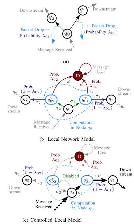
Figure 1: Node centric decision for packet forwarding with non-zero drop probability for all choices

III Modeling Ad-hoc Networks as PFSA

We consider an ad-hoc network of communicating nodes endowed with limited computational resources. For simplicity of exposition, we develop the theoretical results under the assumption of a single sink. This is not a serious restriction and can be easily relaxed. The location and identity of the sink is not known a priori to the individual nodes. Inter-node communication links are assumed to be imperfect, with the possibility of packet drop in each transmission attempt. We assume nodes can efficiently gather the following information:

1. (Set of Neighboring Nodes:) Number and unique id. of nodes to which it can successfully send data via a 1-hop direct link.

2. (Local Link Properties:) Link-specific probability of packet drop for one-way communication to a specific neighbor.

We further assume that the link-specific packet drop probabilities are either constant, or change slowly enough, making it possible to treat them locally as time-invariant constants for route optimization. Note that this does not imply that the network topology is assumed to be static; we only require that the packet-drop probability for communication from any given node $q_{i}$ to a particular neighbor $q_{j}$ be more or less constant, say $0.7$. Thus $q_{i}$ may choose not to send data to $q_{j}$ all the time, but when it does, then, on the average, $70\%$ of the packets get dropped. In practice, the packet drop probabilities may vary with current network condition, $e.g.$ congestion leading to buffer overflow at specific nodes or (in the context of sensor networks) high-traffic nodes running out of power. We do not consider these effects in detail; however we briefly describe strategies to handle such effects via simple modifications of the basic principles laid out under the assumption of constant drop probabilities. Specific applications, such as wireless sensor networks, require routing schemes that in addition to throughput, are aware of energy and power issues. Also, data-priority need to be respected to enable context-aware routing.

First we formalize the modeling of an ad-hoc network as a probabilistic finite state automata.

Definition 8 (Neighbor Map)

If $Q$ is the set of all nodes in the network, then the neighbor map $\mathcal{N}:Q\rightarrow 2^{Q}$ specifies, for each node $q_{i}\in Q$, the set of nodes $\mathcal{N}(q_{i})\subset Q$ (excluding $q_{i}$) to which $q_{i}$ can communicate via a single hop direct link.

Definition 9 (Packet Drop Probability)

The link specific packet drop probability $\lambda_{ij}\in[0,1]$ is defined to be the limiting ratio of the number of packets dropped to the total number of packets sent, in communicating from node $q_{i}$ to node $q_{j}$.

Note that the drop probabilities are not constrained to be symmetric in general, $i.e.$, $\lambda_{ij}\neq\lambda_{ji}$. Also, note that we assume the node-based estimation of these ratios to converge fast enough. We visualize the local network around a node $q_{0}$ in a manner illustrated in Figure 1(a) (shown for two neighbors $q_{1}$ and $q_{2}$). In particular, any packet transmitted from $q_{0}$ for $q_{1}$ has a drop probability $\lambda_{01}$, and the ones transmitted to $q_{2}$ have a drop probability $\lambda_{02}$. To correctly represent this information, we require the notion of virtual nodes ($q^{v}_{01},q^{v}_{02}$ in Figure 1(b)).

Definition 10 (Virtual Node)

Given a node $q_{i}$, and a neighbor $q_{j}\in\mathcal{N}(q_{i})$ with a specified drop probability $\lambda_{ij}$, any transmitted data-packet from $q_{i}$ for $q_{j}$ is assumed to be first delivered to a virtual node $q^{v}_{ij}$, upon which there is either an automatic ($i.e.$ uncontrollable) forwarding to $q_{j}$ with probability $1-\lambda_{ij}$, or a drop with probability $\lambda_{ij}$. The set of all virtual nodes in a network of $Q$ nodes is denoted by $Q^{v}$ in the sequel.

Hence, the total number of virtual nodes is given by:

$$\textrm{{Card}}(Q^{v})=\sum_{i:q_{i}\in Q}\mathcal{N}(q_{i})$$ (3)

And the cardinality of the set of virtual nodes satisfies:

$$0\leqq\textrm{{Card}}(Q^{v})\leqq\textrm{{Card}}(Q)^{2}-\textrm{{Card}}(Q)$$ (4)

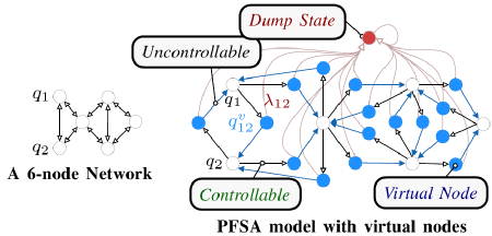
Figure 2: 6-node Network and PFSA model with 23 states (16 virtual nodes, 6 nodes, 1 dump state)

We are ready to model an ad-hoc network as a PFSA.

Definition 11 (PFSA Model of Network)

For a given set of nodes $Q$, the function $\mathcal{N}:Q\rightarrow 2^{Q}$, the link specific drop probabilities $\lambda_{ij}$ for any node $q_{i}$ and a neighbor $q_{j}\in\mathcal{N}(q_{i})$, and a specified sink $q_{\textrm{{Sink}}}\in Q$, the PFSA $\mathds{G}_{\textrm{{N}}}=(Q^{N},\Sigma,\delta,\widetilde{\Pi},\chi,\mathscr{C})$ is defined to be a model of the network, where (denoting $\textrm{{Card}}(\mathcal{N}(q_{i}))=m$):

$$\textrm{\footnotesize$\circ$ States:}\mspace{50.0mu}Q^{N}=Q\bigcup Q^{v}\bigcup\big{\{}q_{D}\big{\}}$$

where $$Q^{v} q_{D} \Sigma$$ is the set of virtual nodes, and is a dump state which models packet loss. For the alphabet :

$$\textrm{\footnotesize$\circ$ Alphabet:}\mspace{50.0mu}\Sigma=\bigcup_{i:q_{i}\in Q}\left(\bigcup_{j:q_{j}\in\mathcal{N}(q_{i})}\sigma_{ij}\right)\bigcup\big{\{}\sigma_{D}\big{\}}$$

$$\sigma_{ij} q_{i} q_{j} \sigma_{D} q_{D}$$ denotes transmission (attempted or actual) from to , and denotes transmission to (packet loss).

$$\hbox{\hbox{\kern 0.0pt\raise-6.24445pt\vbox{\halign{\relax\hfil\txtline@@{#}\hfil\cr\hbox{{\ignorespaces\leavevmode\footnotesize$\circ$ Transition }\\\hbox{{\ignorespaces\footnotesize Map: $\phantom{XXXX.X.}$}\crcr}}}}\ \mspace{5.0mu}\delta(q,\sigma)=\left\{\begin{array}[]{cl}q^{v}_{ij}&\textrm{if }q=q_{i},\sigma=\sigma_{ij}\\ q_{j}&\textrm{if }q=q^{v}_{ij},\sigma=\sigma_{ij}\\ q_{D}&\textrm{if }q=q^{v}_{ij},\sigma=\sigma_{D}\\ q_{D}&\textrm{if }q=q_{D},\sigma=\sigma_{D}\\ -&\textrm{undefined otherwise}\end{array}\right.}}$$

$$\hbox{\hbox{\kern 0.0pt\raise-9.84445pt\vbox{\halign{\relax\hfil\txtline@@{#}\hfil\cr\hbox{{\ignorespaces\leavevmode\footnotesize$\circ$ Probability }\\\hbox{{\ignorespaces\footnotesize Morph $\phantom{XXXXx}$}\\\hbox{{\ignorespaces\footnotesize Matrix:$\phantom{XXXXx}$}\crcr}}}}\mspace{3.0mu}\ \widetilde{\Pi}(q,\sigma)=\left\{\begin{array}[]{cl}\frac{1}{m}&\textrm{if }q=q_{i},\sigma=\sigma_{ij}\\ 1-\lambda_{ij}&\textrm{if }q=q^{v}_{ij},\sigma=\sigma_{ij}\\ \lambda_{ij}&\textrm{if }q=q^{v}_{ij},\sigma=\sigma_{D}\\ 1&\textrm{if }q=q_{D},\sigma=\sigma_{D}\\ 0&\textrm{otherwise}\end{array}\right.}}}$$

$$\hbox{\hbox{\kern 0.0pt\raise-6.33334pt\vbox{\halign{\relax\hfil\txtline@@{#}\hfil\cr\hbox{{\ignorespaces\leavevmode\footnotesize$\circ$ Characteristic }\\\hbox{{\ignorespaces\footnotesize Weights:$\phantom{XXXXXX..}$}\crcr}}}}\mspace{50.0mu}\chi_{i}=\left\{\begin{array}[]{cl}1&\textrm{if }q_{i}=q_{\textrm{{Sink}}}\\ 0&\textrm{otherwise}\end{array}\right.}}$$

$$\hbox{\hbox{\kern 0.0pt\raise-5.51111pt\vbox{\halign{\relax\hfil\txtline@@{#}\hfil\cr\hbox{{\ignorespaces\leavevmode\footnotesize$\circ$ Controllable }\\\hbox{{\ignorespaces\footnotesize Transitions:$\phantom{Xxx}$}\crcr}}}}\mspace{15.0mu}\ \forall q_{i}\in Q,q_{j}\in\mathcal{N}(q_{i}),q_{i}\xrightarrow{\sigma_{ij}}q^{v}_{ij}\in\mathscr{C}}}$$

We note that for a network of $Q$ nodes, the PFSA model may have (almost always has, see Figure 2) a significantly larger number of states. Using Eq. (4):

$$\textrm{{Card}}(Q^{N})=\textrm{{Card}}(Q)+\textrm{{Card}}(Q^{v})+1$$ (6)

$$\Rightarrow\textrm{{Card}}(Q)+1\leqq\textrm{{Card}}(Q^{N})\leqq\textrm{{Card}}(Q)^{2}+1$$ (7)

This state-explosion will not be a problem for the distributed approach developed in the sequel, since we use the complete model $\mathds{G}_{\textrm{{N}}}$ only for the purpose of deriving theoretical guarantees. Note, that Definition 11 generates a PFSA model which can be optimized in a straightforward manner using the language-measure-theoretic technique described in Section II (See [14]) for details). This would yield the optimal routing policy in terms of the disabling decisions at each node that minimize source-to-sink drop probabilities (from every node in the network). To see this explicitly, note that the measure-theoretic approach elementwise maximizes $\lim_{\theta\rightarrow 0^{+}}\theta\big{[}\mathbb{I}-(1-\theta)\Pi\big{]}^{-1}\chi=\mathscr{P}\chi$, where the $i^{th}$ row of $\mathscr{P}$ (denoted as $\wp^{i}$) is the stationary probability vector for the PFSA initialized at state $q_{i}$ (See Proposition 1). Since, the dump state has characteristic $-1$, the sink has characteristic $1$, and all other nodes have characteristic $0$, it follows that this optimization maximizes the quantity $\wp^{i}_{\textrm{{Sink}}}-\wp^{i}_{\textrm{Dump}}$, for every source state or node $q_{i}$ in the network. Note that $\wp^{i}_{\textrm{{Sink}}},\wp^{i}_{\textrm{Dump}}$ are the stationary probabilities of reaching the sink and incurring a packet loss to dump respectively, from a given source $q_{i}$. Thus, maximizing $\wp^{i}_{\textrm{{Sink}}}-\wp^{i}_{\textrm{Dump}}$ for every $q_{i}\in Q$ guarantees that the computed routing policy is indeed optimal in the stated sense. However, the procedure in [14] requires centralized computations, which is precisely what we wish to avoid. The key technical contribution in this paper is to develop a distributed approach to language-measure-theoretic PFSA optimization. In effect, the theoretical development in the next section allows us to carry out the language-measure-theoretic optimization of a given PFSA, in situations where we do not have access to the complete $\Pi$ matrix, or the $\chi$ vector at any particular node ($i.e.$ each node has a limited local view of the network), and are restricted to communicate only with immediate neighbors. We are interested in not just computing the measure vector in a distributed manner, but optimizing the PFSA via selected disabling of controllable transitions (See Section II). This is accomplished by Algorithm 1.

Before we embark up on the detailed analysis of Algorithm 1 in the next section, we briefly elucidate the connection with decentralized Markov Decision Processes. The PFSA based modeling framework is somewhat different from the standard MDP architecture. For example, in contrast to the latter, our actions are ”controllable” transitions, and have probabilities associated with them. Rewards and penalties are not associated with individual actions, but with state visitations (and modeled via the characteristic weights). We maximize the long term or expected reward by maximizing the probability of reaching the sink, while simultaneously minimizing the probability of reaching the dump state, $i.e.$, a drop, from any arbitrary node in the network. More details on relations to the standard approach is given in [18].

IV Decentralized PFSA Optimization

input : $\mathds{G}_{\textrm{{N}}}=(Q,\Sigma,\delta,\widetilde{\Pi},\chi,\mathscr{C})$, $\theta$

begin  Initialize $\forall q_{i}\in Q,\widehat{\nu}^{\textrm{}}_{\theta}|_{i}=0$

$/*\$ Begin Infinite Asynchronous Loop $\ */$ while true do  for each node $q_{i}\in Q$ do  if $\mathcal{N}(q_{i})\neq\varnothing$ then 

$m=\textrm{{Card}}(\mathcal{N}(q_{i}))$

for each node $q_{j}\in\mathcal{N}(q_{i})$ do  $/*\$ (a1) Internode Communication $\ */$ Query $\widehat{\nu}^{\textrm{}}_{\theta}|_{j}$ & Drop Prob. $\lambda_{ij}$

$/*\$ (a2) Control Adaptation $\ */$ if $\widehat{\nu}^{\textrm{}}_{\theta}|_{j}<\widehat{\nu}^{\textrm{}}_{\theta}|_{i}$ then  $\Pi_{ii}=\Pi_{ii}+\Pi_{i(q^{V}_{ij})}$

$\Pi_{i(q^{V}_{ij})}=0$;  /* Disable */

else  if $\Pi_{i(q^{V}_{ij})}==0$ then  $\Pi_{i(q^{V}_{ij})}=\frac{1}{m}$

$\Pi_{ii}=\Pi_{ii}-\frac{1}{m}$ $/*\$ Enable $\ */$ endif endif $/*\$ (a3) Updating Virtual Nodes $\ */$ $\widehat{\nu}^{\textrm{}}_{\theta}|_{(q_{ij}^{V})}=(1-\theta)(1-\lambda_{ij})\widehat{\nu}^{\textrm{}}_{\theta}|_{j}$ endfor endif $/*\$ (a4) Updating Node $\ */$ $\widehat{\nu}^{\textrm{}}_{\theta}|_{i}=\displaystyle\mspace{-25.0mu}\sum_{j:q_{j}\in\mathcal{N}(q_{i})}\mspace{-20.0mu}(1-\theta)\Pi_{i(q^{V}_{ij})}\widehat{\nu}^{\textrm{}}_{\theta}|_{(q_{ij}^{V})}$                            $+(1-\theta)\Pi_{ii}\widehat{\nu}^{\textrm{}}_{\theta}|_{i}+\theta\chi|_{i}$ endforendw end

Algorithm 1 Distributed Update of Node Measures

Notation 4

In the sequel, the current measure value, for a given $\theta$, at node $q_{i}\in Q$ is denoted as $\widehat{\nu}^{\textrm{}}_{\theta}|_{i}$, and the measure of the virtual node $q^{v}_{ij}\in Q^{N}$ is denoted as $\widehat{\nu}^{\textrm{}}_{\theta}|_{(q_{ij}^{V})}$. The parenthesized entry $(q_{ij}^{V})$ denotes the index of the virtual node $q^{v}_{ij}$ in the state set $Q^{N}$. Similarly, the transition probability from $q_{i}$ to $q^{v}_{ij}$ is denoted as $\Pi_{i(q_{ij}^{V})}$. The subscript entry $i(q_{ij}^{V})$ denotes the $ik^{th}$ element of $\Pi$, where $k=(q_{ij}^{V})$.

Algorithm 1 establishes a distributed, asynchronous update procedure which achieves the following:

$$\forall q_{i}\in Q,\widehat{\nu}_{\theta}|_{i}\xrightarrow[\hbox{\hbox{\kern 0.0pt\raise-2.5pt\vbox{\halign{\relax\hfil\txtline@@{#}\hfil\cr\hbox{{\ignorespaces\leavevmode\footnotesize convergence}\crcr}}}}]{\hbox{\hbox{\kern 0.0pt\raise-3.55556pt\vbox{\halign{\relax\hfil\txtline@@{#}\hfil\cr\hbox{{\ignorespaces\leavevmode\footnotesize global }\crcr}}}}}\nu^{\star}_{\theta}|_{i}}}$$ (10)

where $\nu^{\star}_{\theta}|_{i}$ is the optimal measure for $q_{i}\in Q$ that would be obtained by optimizing the PFSA $\mathds{G}_{\textrm{{N}}}$, for a given $\theta$, in a centralized approach (See Section II). The optimal routing policy can then be obtained by forwarding packets to neighboring nodes which have a better or equal current measure value. If more than a one such neighbor is available, then one chooses the forwarding node randomly, in an equiprobable manner. In fact, the nodes need not wait for exact convergence; in the sequel we show that this forwarding policy converges to the globally optimal routing policy, that, for a sufficiently small $\theta$, it maximizes probability of reaching the sink, while simultaneously minimizing the probability of packet drops. Furthermore, choosing randomly between qualifying neighboring nodes leads to significant congestion resilience. These issues would be elaborated in the sequel (Proposition 7). First, Algorithm 1 is analyzed to establish convergence.

Algorithm 1 has four distinct parts, marked as (a1), (a2), (a3) and (a4). Part (a1) involves internode communication, to enable a particular node $q_{i}\in Q$ to ascertain the current measure values of neighboring nodes, and the drop probabilities $\lambda_{ij}$ on respective links. Recall, that we assume the probabilities $\lambda_{ij}$ to be more or less constant; nevertheless nodes estimate these values to adapt to changing (albeit slowly) network conditions. Part (a2) is the control adaptation, in which the nodes decide, based on local information, the set of forwarding nodes. Part (a3) is the computation of the updated measure values for the virtual nodes $q^{v}_{ij}$ where $j:q_{j}\in\mathcal{N}(q_{i})$. Finally, part (a4) updates the measure of the node $q_{i}$ based on the computed current measures of the virtual nodes. We note that Algorithm 1 only uses information that is either available locally, or that which can be queried from neighboring nodes.

Proposition 2 (Convergence)

For a network $Q$ modeled as a PFSA $\mathds{G}_{\textrm{{N}}}=(Q^{N},\Sigma,\delta,\widetilde{\Pi},\chi,\mathscr{C})$, the distributed procedure in Algorithm 1 has the following properties:

1. Computed measure values for every node $q_{i}\in Q$ are non-negative and bounded above by $1$, $i.e.$,

   $$\forall q_{i}\in Q^{N},\forall t\in[0,\infty),\ \widehat{\nu}^{t}_{\theta}|_{i}\in[0,1]$$ (11)

2. For constant drop probabilities and constant neighbor map $\mathcal{N}:Q\rightarrow 2^{Q}$, Algorithm 1 converges in the sense:

   $$\forall q_{i}\in Q^{N},\lim_{t\rightarrow\infty}\widehat{\nu}^{t}_{\theta}|_{i}=\nu^{\infty}_{\theta}|_{i}\in[0,1]$$ (12)

3. Convergent measure values coincide with the optimal values computed by the centralized approach:

   $$\forall q_{i}\in Q^{N},\nu^{\infty}_{\theta}|_{i}=\nu^{\star}_{\theta}|_{i}$$ (13)

Proof:

(Statement 1:) Non-negativity of the measure values is obvious. For establishing the upper bound, we use induction on computation time $t$. We note that all the measure values $\widehat{\nu}^{t}_{\theta}|_{i}$ are initialized to $0$ at time $t=0$. The first node to change its measure will be the sink, which is updated at some time $t=t_{0}$:

$$\widehat{\nu}^{t_{0}}_{\theta}|_{(q_{\textrm{{Sink}}})}=0+\theta\chi_{(q_{\textrm{{Sink}}})}=\theta$$ (14)

where the first term is zero since all nodes still have measure zero and the sink characteristic $\chi_{(q_{\textrm{{Sink}}})}=1$. Thus, there exists a non-trivial time instant $t_{0}$, at which:

$$\textrm{{\small(Induction Basis)} }\forall q_{i}\in Q^{N},\widehat{\nu}^{t}_{\theta}|_{i}\leqq 1$$ (15)

Next we assume for time $t=t^{\prime}$, we have

$$\textrm{{\small(Induction Hypothesis)} }\forall q_{i}\in Q^{N},\forall\tau\leqq t^{\prime},\widehat{\nu}^{\tau}_{\theta}|_{i}\leqq 1$$

We consider the next updates for physical nodes and virtual nodes separately, and denote the time instant for the next updates as $t^{\prime}_{+}$. Note, that $t^{\prime}_{+}$ actually may be different for different nodes (asynchronous operation).
(Virtual Nodes) For any virtual node $q_{i}=q^{v}_{kj}\in Q^{N}$, where $q_{k},q_{j}\in Q$, we have:

$$\widehat{\nu}^{t^{\prime}_{+}}_{\theta}|_{i}=(1-\lambda_{ij})(1-\theta)\widehat{\nu}^{t^{\prime}}_{\theta}|_{j}\leqq 1$$ (16)

(Physical Nodes) For any $q_{i}\in Q$, where set of enabled neighbors $E_{n}=\big{\{}q_{j}\in\mathcal{N}(q_{i})\ \textrm{s.t. }\widehat{\nu}^{t^{\prime}_{+}}_{\theta}|_{(q_{ij}^{V})}\geqq\widehat{\nu}^{t^{\prime}}_{\theta}|_{i}\big{\}}$:

$$\widehat{\nu}^{\tau+}_{\theta}|_{i}=\frac{1}{\textrm{{Card}}(\mathcal{N}(q_{i}))}\bigg{(}\sum_{j:q_{j}\in E_{n}}(1-\theta)^{2}(1-\lambda_{ij})\widehat{\nu}^{t^{\prime}}_{\theta}|_{(q_{ij}^{V})}\\ +\sum_{j:j\in\mathcal{N}(q_{i})\setminus E_{n}}(1-\theta)\widehat{\nu}^{t^{\prime}}_{\theta}|_{i}\bigg{)}\\ \leqq\frac{1}{\textrm{{Card}}(\mathcal{N}(q_{i}))}\bigg{(}\sum_{j:q_{j}\in E_{n}}1+\sum_{j:j\in\mathcal{N}(q_{i})\setminus E_{n}}1\bigg{)}\leqq 1$$

which establishes Statement 1.
(Statement 2:) We claim that for each node $q_{i}\in Q^{N}$, the sequence of measures $\widehat{\nu}^{t}_{\theta}|_{i}$ forms a monotonically non-decreasing sequence as a function of the computation time $t$. Again, we use induction on computation time. Considering the time instant $t_{0}$ (See Eqn. (14)), we note that we have an instant up to which all measure values have indeed changed in a non-decreasing fashion, since the measure of $q_{\textrm{{Sink}}}$ increased to $\theta$, while other nodes are still at $0$; which establishes the basis. For our hypothesis, we assume that there exists some time instant $t^{\prime}>t_{0}$, such that all measure values have undergone non-decreasing updates up to $t^{\prime}$. We consider the physical node $q_{i}\in Q$ which is the first one to update next, say at the instant $t^{\prime}_{+}>t^{\prime}$. Referring to Algorithm 1, this update occurs by first updating the set of virtual nodes $\{q_{ij}^{v}:q_{j}\in\mathcal{N}(q_{i})\}$. Since virtual nodes update as:

$$\widehat{\nu}^{t^{\prime}_{+}}_{\theta}|_{(q^{v}_{ij}}=(1-\theta)(1-\lambda_{ij})\widehat{\nu}^{t^{\prime}}_{\theta}|_{j}$$ (17)

it follows from the induction hypothesis that

$$\widehat{\nu}^{t^{\prime}_{+}}_{\theta}|_{(q^{v}_{ij})}\geqq\widehat{\nu}^{t^{\prime}}_{\theta}|_{(q^{v}_{ij})}$$ (18)

If the connectivity ($i.e.$ the forwarding decisions) for the physical node $q_{i}$ remains unchanged for the instants $t^{\prime}$ and $t^{\prime}_{+}$, and since the measures of any neighboring node has not decreased (by induction hypothesis), then:

$$\widehat{\nu}^{t^{\prime}_{+}}_{\theta}|_{i}\geqq\widehat{\nu}^{t^{\prime}}_{\theta}|_{i}$$ (19)

If, on the other hand, the set of disabled transitions for $q_{i}$ changes ($e.g.$ for some $q_{j}\in\mathcal{N}(q_{i})$, $q_{i}\xrightarrow{\sigma_{ij}}q_{ij}^{v}$ was disabled at $t^{\prime}$ and is enabled at $t^{\prime}_{+}$, or vice verse), the measure of node $q_{i}$ is increased by the additive factor $\frac{(1-\theta)}{\textrm{{Card}}(\mathcal{N}(q_{i}))}\bigg{|}\widehat{\nu}^{t^{\prime}}_{\theta}|_{i}-\widehat{\nu}^{t^{\prime}}_{\theta}|_{(q^{v}_{ij})}\bigg{|}$, which completes the inductive process and establishes our claim that the measure values form a non-decreasing sequence for each node as a function of the computation time. Since, a non-decreasing bounded sequence in a complete space must converge to a unique limit [17], the convergence:

$$\forall q_{i}\in Q^{N},\lim_{t\rightarrow\infty}\widehat{\nu}^{t}_{\theta}|_{i}=\nu^{\infty}_{\theta}|_{i}\in[0,1]$$ (20)

follows from the existence of the upper bound established in Statement 1. This establishes Statement 2.
(Statement 3:) From the update equations in Algorithm 1, we note that the limiting measure values satisfy:

$$\widehat{\nu}_{\theta}^{\infty}\big{|}_{i} =(1-\theta)\sum_{j\in\mathcal{N}(i)}\Pi_{ij}\widehat{\nu}_{\theta}^{\infty}\big{|}_{j}+\theta\chi|_{i}$$

$$\Rightarrow\widehat{\nu}_{\theta}^{\infty} =\theta\big{[}\mathbb{I}-(1-\theta)\Pi\big{]}^{-1}\chi$$ (21)

which implies that measure values does indeed converge to the measure vector computed in a centralized fashion (See Eq. (1)). Noting that any further disabling (or re-enabling) would not increase the measure values computed by Algorithm 1, we conclude that this must be the optimal disabling set that would be obtained by the centralized language-measure theoretic optimization of PFSA $\mathds{G}_{\textrm{{N}}}$ (Section II). This completes the proof. ∎

Proposition 3 (Initialization Independence)

For a network $Q$ modeled as a PFSA $\mathds{G}_{\textrm{{N}}}=(Q^{N},\Sigma,\delta,\widetilde{\Pi},\chi,\mathscr{C})$, convergence of Algorithm 1 is independent of the initialization of the measure values, $i.e.$, if $\widehat{\nu}_{\theta,\alpha}^{t}$ denotes the measure vector at time $t$ with arbitrary initialization $\alpha\in[0,1]^{\textrm{{Card}}(Q^{N})}$, then:

$$\lim_{t\rightarrow\infty}\widehat{\nu}_{\theta,\alpha}^{t}=\lim_{t\rightarrow\infty}\widehat{\nu}_{\theta}^{t}$$ (22)

where $\widehat{\nu}_{\theta,\alpha}^{0}=\alpha$ and $\widehat{\nu}_{\theta}^{0}=[0\cdots 0]^{T}$.

Proof:

The measure update equations in Algorithm 1 dictate that the measure values will have a positive contribution from $\alpha$. Denoting the contribution of $\alpha$ to the measure of node $q_{i}\in Q$ at time $t$ as $\mathcal{C}^{t}_{\alpha}(q_{i})$, we note that the measure can be written as $\widehat{\nu}_{\theta,\alpha}^{t}=\mathcal{C}^{t}_{\alpha}(q_{i})+f_{i}^{t}$, where $f_{i}^{t}$ is independent of $\alpha$. Furthermore, the linearity of the updates imply that $\mathcal{C}^{t}_{\alpha}(q_{i})$ can be used to formulate an inductive argument as follows. We use $k_{\star}^{t}\in\mathbb{N}\cup\{0\}$ to denote the minimum number of updates that every node in the network has encountered up to time instant $t\in[0,\infty)$. We claim that:

$$\forall q_{i}\in Q,\forall t\in[0,\infty),\mathcal{C}^{t}_{\alpha}(q_{i})\leqq(1-\theta)^{k_{\star}^{t}}||\alpha||_{1}$$ (23)

To establish this claim, we use induction on $k_{\star}^{t}$. For the basis, we note that there exists a time instant $t_{0}$, such that $\forall\tau\leqq t_{0},k_{\star}^{\tau}=0$, implying that

$$\forall\tau\leqq t_{0},\mathcal{C}^{\tau}_{\alpha}(q_{i})=\alpha_{i}\leqq(1-\theta)^{0}\sum_{q_{j}\in Q}\alpha_{j}=(1-\theta)^{k_{\star}^{\tau}}||\alpha||_{1}$$

We assume that if at some $t_{k}$, $k_{\star}^{t_{k}}=k\in\mathbb{N}$, then:

$$\textrm{{\small(Induction Hypothesis)} }\forall q_{i}\in Q,\mathcal{C}^{t_{k}}_{\alpha}(q_{i})\leqq(1-\theta)^{k}||\alpha||_{1}$$

Next let $q_{i}\in Q$ be an arbitrary physical node, and we consider the first update of $q_{i}$ at $t_{k}^{+}>t_{k}$:

$$\widehat{\nu}^{t_{k}^{+}}_{\theta}|_{i}=\mspace{-25.0mu}\sum_{j:q_{j}\in\mathcal{N}(q_{i})}\mspace{-20.0mu}(1-\theta)\Pi_{i(q^{v}_{ij})}\widehat{\nu}^{t_{k}}_{\theta}|_{(q_{ij}^{v})}+(1-\theta)\Pi_{ii}\widehat{\nu}^{t_{k}}_{\theta}|_{i}+\theta\chi_{i}\\ \Rightarrow\mathcal{C}^{t_{k}^{+}}_{\alpha}(q_{i})\leqq\mspace{-28.0mu}\sum_{j:q_{j}\in\mathcal{N}(q_{i})}\mspace{-20.0mu}(1-\theta)\Pi_{i(q^{v}_{ij})}(1-\lambda_{ij})(1-\theta)(1-\theta)^{k}||\alpha||_{1}\\ +(1-\theta)\Pi_{ii}(1-\theta)^{k}||\alpha||_{1}+\theta\chi_{i}\\ \Rightarrow\mathcal{C}^{t_{k}^{+}}_{\alpha}(q_{i})\leqq(1-\theta)^{k+1}||\alpha||_{1}\mspace{325.0mu}$$

We note that if $k_{\star}^{t_{k+1}}=k+1$, then every node $q_{i}\in Q$ must have undergone one more update since $t_{k}$ implying:

$$\forall q_{i}\in Q,\mathcal{C}^{t_{k+1}}_{\alpha}(q_{i})\leqq(1-\theta)^{k+1}||\alpha||_{1}$$ (24)

which completes the induction proving Eq. (23). Observing that $\lim_{t\rightarrow\infty}k_{\star}^{t}=\infty$, and $||\alpha||_{1}<\infty$, we conclude:

$$\forall q_{i}\in Q,\lim_{t\rightarrow\infty}\mathcal{C}^{t}_{\alpha}(q_{i})=0$$ (25)

which immediately implies Eq. (22). ∎

Next we investigate the performance of the proposed approach, and establish guarantees on global performance achieved via local decisions dictated by Algorithm 1. We need some technical lemmas, and the notion of strongly absorbing graphs, and graph powers.

Definition 12 (Exact Power of Graph)

For a given graph $G=(V,E)$, the exact power $G^{d}$, for $d\in\mathbb{N}$, is a graph $(V,E^{\prime})$, such that $(q_{i},q_{j})$ is an edge in $G^{d}$, only if there exists a sequence of edges of length exactly $d$ from node $q_{i}$ to node $q_{j}$ in $G$.

Definition 13 (Strongly Absorbing Graph)

A finite directed graph $G=(V,E)$ ($V$ is the set of nodes and $E\subseteq V\times V$ the set of edges) is defined to be strongly absorbing (SA), if:

1. There are one or more absorbing nodes, $i.e.$, $\exists A\subsetneqq V$, s.t. every node in $A$ (non-empty) is absorbing.

2. There exists at least one sequence of edges from any node to one of the absorbing nodes in $A$.

3. If $E^{d}$ denotes the set of edges for the $d^{th}$ exact power of $G$, then, for distinct nodes $q_{i},q_{j}\in V$,

   $$(q_{i},q_{j})\in E\Rightarrow\forall d\in\mathbb{N},\ (q_{j},q_{i})\notin E^{d}$$ (26)

Lemma 1 (Properties of SA Graphs)

Given a SA graph $G=(V,E)$, with $A\subsetneqq V$ the absorbing set:

1. The power graph $G^{d}$ is SA for every $d\in\mathbb{N}$.

2. $q\notin A\Rightarrow\exists q^{\prime}\in V\setminus\{q\}\ \textrm{s.t.}\ (q^{\prime},q)\notin E$

3. $\exists d\in\mathbb{N}\left(\forall q\in V\setminus A\left(\exists q^{\prime}\in A\left((q,q^{\prime})\in E^{d}\right)\right)\right)$

Proof:

Statement 1 is immediate from Definition 13. Statement 2 follows immediately from noting:

$$q\notin A\Rightarrow\exists q^{\prime}\in V\setminus\{q\}\ \textrm{s.t.}\ (q,q^{\prime})\in E\Rightarrow(q^{\prime},q)\notin E$$

Statement 3 follows, since from each node there is a path (length bounded by $\textrm{{Card}}(V)$) to a absorbing state. ∎

The performance of such control policies, and particularly the convergence time-complexity is closely related to the spectral gap of the induced Markov Chains. Hence we need to compute lower bounds on the spectral gap of the chains arising in the context of the proposed optimization, which (as we shall see later) have the strongly absorbing property. The following result computes such a bound as a simple function of the non-unity diagonal entries of $\Pi$.

Proposition 4 (Spectral Bound)

Given a n-state PFSA $G=(Q,\Sigma,\delta,\widetilde{\Pi})$ with a strongly absorbing graph, the magnitude of non-unity eigenvalues of the transition matrix $\Pi$ is bounded above by the maximum non-unity diagonal entry of $\Pi$.

Proof:

Without loss of generality, we assume that $G$ has a single absorbing state (distinct absorbing states can be merged without affecting non-unity eigenvalues). Now, $\mu$ is an eigenvalue of $\Pi$ iff $\mu^{d}$ is an eigenvalue of $\Pi^{d},d\in\mathbb{N}$. From Lemma 1:

• $\exists\ell\in\mathbb{N}$ s.t. $\Pi^{\ell}$ has no zero entry in column corresponding to the absorbing state. Let $d_{\star}$ be the smallest such integer.

• Every non-absorbing state has at least one zero element in the corresponding column of $\Pi^{d_{\star}}$.

• Statements C1,C2 are true for any integer $d\geqq d_{\star}$.

We denote the column of ones as $\mathbf{e}$, $i.e.$, $\mathbf{e}=[1\cdots 1]^{T}$ Since $\Pi^{d}$ is (row) stochastic, we have $\Pi^{d}\mathbf{e}=\mathbf{e}$. Hence, if $v$ is a left eigenvector for $\Pi^{d}$ with eigenvalue $\mu^{d}$, then:

$$v\Pi^{d}\mathbf{e}=v\mathbf{e}=\mu^{d}v\mathbf{e}\Rightarrow(1-\mu^{d})v\mathbf{e}=0$$ (27)

implying that if $\mu^{d}\neq 1$, then $v\mathbf{e}=0$. Now we construct $\mathds{C}=[C_{1}\cdots C_{n}]$, where $C_{j}=\min_{j}\Pi^{d}_{ij}$ (minimum column element). Considering the matrix $M=\Pi^{d}-\mathbf{e}\mathds{C}$, we note:

$$(v\Pi^{d}=\mu^{d}v)\wedge(\mu^{d}\neq 1)\Rightarrow vM=\mu^{d}v$$ (28)

Recalling that stationary probability vectors (Perron vectors) of stochastic matrices add up to unity, we have:

$$(v\Pi^{d}=v)\Rightarrow vM=v-v\mathbf{e}\mathds{C}=v-\mathds{C}$$ (29)

which, along with the fact that since $\mathds{C}$ is not a column of all zeros, implies that an upper bound on the magnitudes of the eigenvalues of $M$ provides an upper bound on the magnitude of non-unity eigenvalues for $\Pi^{d}$. Now, invoking the Gerschgorin Circle Theorem [19, 20], we get:

$$|\mu^{d}|\leqq 1-\sum_{j}C_{j}=1-C_{a}\Rightarrow|\mu|\leqq\left(1-C_{a}\right)^{\frac{1}{d}}$$ (30)

where $C_{a}$ is the minimum column element corresponding to the absorbing state. $1-C_{a}$ is the maximum probability of not reaching the absorbing state after $d$ steps from any state, which is bounded above by $(a)^{d_{1}}(b)^{d-d_{1}}$ where $a$ is the maximum non-diagonal entry in $\Pi$ not going to the absorbing state, $b$ is the maximum of the non-unity diagonal entries in $\Pi$, and $d_{1}$ is a bounded integer. Since any sequence of non-selfloops is absorbed in a finite number of steps (strongly absorbing property), we have a finite bound for $d_{1}$. Hence we have:

$$|\mu|\leqq\lim_{d\rightarrow\infty}a^{\frac{d_{1}}{d}}b^{1-\frac{d_{1}}{d}}=b=\max_{q_{i}:\Pi_{ii}<1}\Pi_{ii}$$ (31)

This completes the proof. ∎

Next, we make rigorous our notion of policy performance, and near-global or $\epsilon$-optimality.

Definition 14 (Policy Performance & $\epsilon$-Optimality)

The performance vector $\rho^{S}$ of a given routing policy $S$ is the vector of node-specific probabilities of a packet eventually reaching the sink. A policy $U$ has Utopian performance if its performance vector (denoted as $\rho^{U}$) element-wise dominates the one for any arbitrary policy $S$, $i.e.$ $\forall q_{i}\in Q^{N},\rho^{U}_{i}\geqq\rho^{S}_{i}$. A policy $P$ has $\epsilon$-optimal performance, if for some given $\epsilon>0$, we have:

$$||\rho^{P}-\rho^{U}||_{\infty}\leqq\epsilon$$ (32)

For a chosen $\theta$, the limiting policy $P_{\theta}$ computed by Algorithm 1 results in element-wise maximization of the measure vector over all possible supervision policies (where supervision is to be understood in the sense of the defined control philosophy). $\widehat{\nu}^{\infty}_{\theta}$ is related to the policy performance vector $\rho^{P_{\theta}}$ as follows. Selective disabling of the transitions dictated by the policy $P_{\theta}$ induces a controlled PFSA, which represents the optimally supervised network, for a given $\theta$. Let the transition matrix for this optimized PFSA be $\Pi^{\star}_{\theta}$, and its Cesaro limit be $\mathscr{P}^{\star}_{\theta}$. (Note: $\Pi^{\star}_{\theta}$, $\mathscr{P}^{\star}_{\theta}$ are stochastic matrices.) Then:

$$\forall q_{i}\in Q^{N},\mathscr{P}^{\star}_{\theta}\chi\big{|}_{i,(q_{\textrm{{Sink}}})}=\rho^{P_{\theta}}_{i}$$ (33)

In the sequel, we would need to distinguish between the optimal measure vector $\widehat{\nu}^{\infty}_{\theta^{\prime}}$ (optimal for a given $\theta=\theta^{\prime}$) computed by Algorithm 1, and the one obtained by first computing $\widehat{\nu}^{\infty}_{\theta^{\prime}}$ and then using the PFSA structure obtained in the process to compute the measure vector for some other value of $\theta=\theta^{\prime\prime}$. These two vectors may not be identical.

Notation 5

In the sequel, we denote the vector obtained in the latter case as $\widehat{\nu}^{\infty}_{\left(\theta^{\prime},\theta^{\prime\prime}\right)}$ implying that we have $\widehat{\nu}^{\infty}_{\left(\theta,\theta\right)}=\widehat{\nu}^{\infty}_{\theta}$.

Lemma 2

We have the following equalities:

$$\lim_{\theta\rightarrow 0^{+}}\widehat{\nu}^{\infty}_{\left(\theta^{\prime},\theta\right)}=\rho^{P_{\theta^{\prime}}}$$ (34a)

$$\lim_{\theta\rightarrow 0^{+}}\widehat{\nu}^{\infty}_{\left(\theta,\theta\right)}=\rho^{U}$$ (34b)

Proof:

Recalling Eq. (33), and noting that for any PFSA with transition matrix $\Pi$ (with Cesaro limit $\mathscr{P}$), we have $\lim_{\theta\rightarrow 0^{+}}\widehat{\nu}_{\theta}=\lim_{\theta\rightarrow 0^{+}}\theta\big{[}\mathbb{I}-(1-\theta)\Pi\big{]}^{-1}\chi=\mathscr{P}\chi$, we have Eq. (34a). In general, different choices of $\theta$ result in different disabling decisions, and hence different policies. However, since there is at most a finite number of distinct policies for a finite network, there must exist a $\theta_{\star}$ such that for all choices $0<\theta\leqq\theta_{\star}$, the policy remains unaltered (although the measure values may differ). Since, executing the optimization with vanishingly small $\theta$ yields a performance vector identical (in the limit) with the optimal measure vector element-wise dominating the one for any arbitrary policy, the policy obtained for $0<\theta\leqq\theta_{\star}$ has Utopian performance. Hence:

$$\lim_{\theta\rightarrow 0^{+}}\widehat{\nu}^{\infty}_{\left(\theta,\theta\right)}=\lim_{\theta\rightarrow 0^{+}}\widehat{\nu}^{\infty}_{\left(\theta_{\star},\theta\right)}=\rho^{P_{\theta_{\star}}}=\rho^{U}$$ (35)

This completes the proof. ∎

Computation of the critical $\theta_{\star}$ is non-trivial from a distributed perspective, although centralized approaches have been reported [14]. Thus it is hard to guarantee Utopian performance in Algorithm 1. Also, $\theta_{\star}$ may be too small resulting in an unacceptably poor convergence rate. Nevertheless, we will show that, given any $\epsilon>0$, one can choose $\theta$ to guarantee $\epsilon$-optimal performance of the limiting policy in the sense of Definition 14. We would need the following result.

Lemma 3

Given any PFSA, with transition matrix $\Pi$ and corresponding Cesaro limit $\mathscr{P}$, and $\mu$ being a non-unity eigenvalue of $\Pi$ with maximal magnitude, we have:

$$\big{|}\big{|}\theta\big{[}\mathbb{I}-(1-\theta)\Pi\big{]}^{-1}-\mathscr{P}\big{|}\big{|}_{\infty}\leqq\frac{\theta}{1-|\mu|}$$ (36a)

$$\big{|}\big{|}\nu_{(\theta,\theta)}-\lim_{\theta^{\prime}\rightarrow 0^{+}}\nu_{(\theta,\theta^{\prime})}\big{|}\big{|}_{\infty}\leqq\frac{\theta||\chi||_{\infty}}{1-|\mu|}$$ (36b)

Proof:

Denoting $M=\big{[}\mathbb{I}-(1-\theta)\Pi\big{]}^{-1}-\frac{1}{\theta}\mathscr{P}$,

$$\textstyle M= [\mathbb{I}-(1-\theta)\Pi]^{-1}-\mathscr{P}\sum_{k=0}^{\infty}(1-\theta)^{k}$$

$$\textstyle= \sum_{k=0}^{\infty}(1-\theta)^{k}(\Pi-\mathscr{P})^{k}-\mathscr{P}$$

$$= [\mathbb{I}-(1-\theta)(\Pi-\mathscr{P})]^{-1}-\mathscr{P}$$

We note, that if $u$ is a left eigenvector of $\Pi$ with unity eigenvalue, then $u\mathscr{P}=u$. Also, if the eigenvalue corresponding to $u$ is strictly within the unit circle, then $u\mathscr{P}=0$. After a little algebra, it follows that if $u$ is the left eigenspace (denoted as $E(1)$) corresponding to unity eigenvalues of $\Pi$, then $uM=0$, otherwise, $uM=\frac{1}{1-(1-\theta)\mu}u$, where $\mu$ is a non-unity eigenvalue for $\Pi$. Invoking the definition of induced matrix norms, and noting $||A||_{\infty}=||A^{T}||_{1}$ for any square matrix $A$:

$$||M||_{\infty}=\max_{||u||_{1}=1}||uM||_{1}=\max_{||u||_{1}=1\wedge u\notin E(1)}||uM||_{1}$$ (37)

We further note that since $[\mathbb{I}-(1-\theta)(\Pi-\mathscr{P})]^{-1}$ is guaranteed to be invertible [14], its eigenvectors form a basis, implying:

$$\textstyle u=\sum_{j}c_{j}u^{j},\ \textrm{with}\ \left|\left|\sum_{j}c_{j}u^{j}\right|\right|_{1}=1$$ (38)

where $u^{j}$ are eigenvectors of $[\mathbb{I}-(1-\theta)(\Pi-\mathscr{P})]^{-1}$ with non-unity eigenvalues, and $c_{j}$ are complex coefficients. An upper bound for $||M||_{1}$ can be now computed as:

$$\textstyle||M||_{\infty}\leqq\frac{1}{1-(1-\theta)|\mu|}\left|\left|\sum_{j}c_{j}u^{j}\right|\right|_{1}=\frac{1}{1-(1-\theta)|\mu|}\leqq\frac{1}{1-|\mu|}$$

where $\mu$ is a non-unity eigenvalue for $\Pi$ with maximal magnitude. This establishes Eq. (36a). Finally, noting:

$$\nu_{(\theta,\theta)}-\lim_{\theta^{\prime}\rightarrow 0^{+}}\nu_{(\theta,\theta^{\prime})}=\big{(}\theta[\mathbb{I}-(1-\theta)\Pi]^{-1}-\mathscr{P}\big{)}\chi$$

establishes Eq. (36b). ∎

The next proposition the key result relating a specific choice of $\theta$ to guaranteed $\epsilon$-optimal performance.

Proposition 5 (Global $\epsilon$-Optimality)

Given any $\epsilon>0$, choosing $\theta=\left.\epsilon\right/m^{2}\ \textrm{where}\ m=\max_{q\in Q}\textrm{{Card}}(\mathcal{N}(q))$ guarantees that the limiting policy computed by Algorithm 1 is $\epsilon$-optimal in the sense of Definition 14.

Proof:

We observe that the limiting measure values $\widehat{\nu}^{\infty}_{\theta}|_{i}=\nu^{\star}_{\theta}|_{i}$ computed by Algorithm 1 can be represented by convergent sums of the form ($a_{ij}$ are non-negative reals):

$$\forall q_{i}\in Q^{N},\ \widehat{\nu}^{\infty}_{\theta}|_{i}=\sum_{j=1}^{\infty}a_{ij}(1-\theta)^{j}$$ (39)

implying that for each $q_{i}\in Q$, $\widehat{\nu}^{\infty}_{\left(\theta,\theta_{1}\right)}|_{i}$ (See Notation 5) is a monotonically decreasing function of $\theta_{1}$ in the domain $[0,\theta]$. We note that if the following statement:

$$\forall q_{i},q_{j}\in Q^{N},$$

$$\widehat{\nu}^{\infty}_{\theta}|_{i}>\widehat{\nu}^{\infty}_{\theta}|_{j}\Rightarrow\forall\theta_{1}\leqq\theta,\ \widehat{\nu}^{\infty}_{\left(\theta,\theta_{1}\right)}|_{i}>\widehat{\nu}^{\infty}_{\left(\theta,\theta_{1}\right)}|_{j}$$

is true, then we have Utopian performance for policy $P_{\theta}$, $i.e.$, $\rho^{P_{\theta}}=\rho^{U}$. Hence, if $\rho^{P_{\theta}}\neq\rho^{U}$, then we must have:

$$\exists\theta_{2}<\theta,\exists q_{i},q_{j}\in Q^{N},$$

$$\big{(}\widehat{\nu}^{\infty}_{\theta}|_{i}>\widehat{\nu}^{\infty}_{\theta}|_{j}\big{)}\wedge\big{(}\widehat{\nu}^{\infty}_{\left(\theta,\theta_{1}\right)}|_{i}>\widehat{\nu}^{\infty}_{\left(\theta,\theta_{1}\right)}|_{j}\big{)}$$

upon which Eq. (39), along with the bound established in Eq. (36a), guarantees that if $q_{i},q_{j}$ are nodes (in consecutive order) that satisfy the above statement, then:

$$\lim_{\theta_{1}\rightarrow 0^{+}}\left(\widehat{\nu}^{\infty}_{\left(\theta,\theta_{1}\right)}|_{i}-\widehat{\nu}^{\infty}_{\left(\theta,\theta_{1}\right)}|_{j}\right)\leqq\beta_{\theta}\theta$$ (40)

where $\beta_{\theta}=\frac{1}{1-|\mu|}$, with $\mu$ being a maximal non-unity eigenvalue of the transition matrix of the PFSA computed by Algorithm 1 at $\theta$. Next we claim:

$$\forall\theta^{\prime}\in(0,\theta],\ ||\widehat{\nu}^{\infty}_{\theta^{\prime}}-\widehat{\nu}^{\infty}_{\left(\theta,\theta^{\prime}\right)}||_{\infty}\leqq m^{2}\theta$$ (41)

We observe that, for any $\theta^{\prime}$, the optimal policy $P_{\theta^{\prime}}$ can be obtained by beginning with the PFSA induced by $P_{\theta}$ (which is the optimal policy at $\theta$), and then executing the centralized iterative approach [14], resulting in a sequence of element-wise non-decreasing measure vectors converging to the optimal $\widehat{\nu}^{\infty}_{\theta^{\prime}}$:

$$\widehat{\nu}^{\infty}_{\left(\theta,\theta^{\prime}\right)}=\nu^{[0]}_{\theta^{\prime}}>\nu^{[1]}_{\theta^{\prime}}>\nu^{[2]}_{\theta^{\prime}}>\cdots\nu^{[k^{\star}]}_{\theta^{\prime}}=\widehat{\nu}^{\infty}_{\theta^{\prime}}$$ (42)

where $\nu^{[k]}_{\theta^{\prime}}$ is the vector obtained after the $k^{th}$ iteration, and $k^{\star}<\infty$ is the number of required iterations. Since, $\nu^{[k]}_{\theta^{\prime}}=\theta^{\prime}\big{[}\mathbb{I}-(1-\theta^{\prime})\Pi^{[k]}\big{]}^{-1}\chi$, where the transition matrix after $k^{th}$ iteration is $\Pi^{[k]}$ and setting $\Delta^{[k]}_{\theta^{\prime}}=\nu^{[k]}_{\theta^{\prime}}-\widehat{\nu}^{\infty}_{\left(\theta,\theta^{\prime}\right)}$ we have:

$$\Delta^{[k]}_{\theta^{\prime}}=(1-\theta^{\prime})\big{[}\mathbb{I}-(1-\theta^{\prime})\Pi^{[k]}\big{]}^{-1}(\Pi^{[k]}-\Pi^{[0]})\widehat{\nu}^{\infty}_{\left(\theta,\theta^{\prime}\right)}$$

$$={\textstyle\frac{1-\theta^{\prime}}{\theta^{\prime}}}\big{\{}{\color[rgb]{.545,0,0}\underbrace{\color[rgb]{0,0,0}\theta^{\prime}\big{[}\mathbb{I}-(1-\theta^{\prime})\Pi^{[k]}\big{]}^{-1}}_{\color[rgb]{.545,0,0}\mathds{B}^{[k]}_{\theta^{\prime}}}}\big{\}}\big{\{}{\color[rgb]{.545,0,0}\underbrace{\color[rgb]{0,0,0}(\Pi^{[k]}-\Pi^{[0]})\widehat{\nu}^{\infty}_{\left(\theta,\theta^{\prime}\right)}}_{\color[rgb]{.545,0,0}\omega^{[k]}_{\theta^{\prime}}}}\big{\}}\vspace{-15pt}$$

For $q_{i}\in Q$, let ${\mathds{U}}_{i}^{(0\rightarrow k)}$ be the set of transitions $(q_{i}\xrightarrow{\sigma}q_{j})$, which are updated ($i.e.$ enabled if disabled or vice verse) to go from the configuration corresponding to $\nu^{[0]}_{\theta^{\prime}}$ to the one corresponding to $\nu^{[k]}_{\theta^{\prime}}$. We note that:

$$\mathds{U}_{i}^{(0\rightarrow k)}=\left(\mathds{U}_{i}^{(0\rightarrow 1)}\cap\mathds{U}_{i}^{(0\rightarrow k)}\right)\bigcup\mathscr{W}$$

where $\mathscr{W}=\mathds{U}_{i}^{(0\rightarrow k)}\setminus\left(\mathds{U}_{i}^{(0\rightarrow 1)}\cap\mathds{U}_{i}^{(0\rightarrow k)}\right)$. The $i^{th}$ row of $\Pi^{[1]}$ is obtained from $\Pi^{[0]}$ [14] by disabling controllable transitions $q_{i}\xrightarrow{\sigma}q_{j}$ if $\nu^{[0]}_{\theta^{\prime}}|_{j}>\nu^{[0]}_{\theta^{\prime}}|_{i}$ (and enabling otherwise), and each such update leads to a positive contribution in the corresponding row of $\omega^{[1]}_{\theta^{\prime}}$. It follows that updating any transition $t\equiv(q_{i}\xrightarrow{\sigma}q_{j})\in\left(\mathds{U}_{i}^{(0\rightarrow 1)}\cap\mathds{U}_{i}^{(0\rightarrow k)}\right)$ leads to a positive contribution to $\omega^{[k]}_{\theta^{\prime}}|_{i}$, given by:

$$C_{t}=\widetilde{\Pi}(q_{i},\sigma)\left|\nu^{[0]}_{\theta^{\prime}}\big{|}_{i}-\nu^{[0]}_{\theta^{\prime}}\big{|}_{j}\right|$$ (43)

and for every transition $t^{\prime}\equiv(q_{i}\xrightarrow{\sigma^{\prime}}q_{k})\in\mathscr{W}$ leads to a negative contribution to $\omega^{[k]}_{\theta^{\prime}}|_{i}$, given by:

$$C_{t^{\prime}}=-\widetilde{\Pi}(q_{i},\sigma^{\prime})\left|\nu^{[0]}_{\theta^{\prime}}\big{|}_{i}-\nu^{[0]}_{\theta^{\prime}}\big{|}_{k}\right|$$ (44)

$$\mspace{-90.0mu}\textrm{implying that:}\mspace{13.0mu}\omega^{[k]}_{\theta^{\prime}}|_{i}\leqq\mspace{-140.0mu}\sum_{\mspace{180.0mu}r\in\left(\mathds{U}_{i}^{(0\rightarrow 1)}\bigcap\mathds{U}_{i}^{(0\rightarrow k)}\right)}\mspace{-140.0mu}C_{r}\mspace{92.0mu}$$ (45)

$$\Rightarrow\omega^{[k]}_{\theta^{\prime}}|_{i}\leqq\sum_{\sigma\in\Sigma}\widetilde{\Pi}(q_{i},\sigma)\beta_{\theta}\theta=\beta_{\theta}\theta\mspace{20.0mu}\textrm{(See Eq.~{}\eqref{eqbnd11})}$$

Since the rows corresponding to the absorbing states have no controllable transitions, absorbing states must remain absorbing through out the iterative sequence, and the corresponding entries in $\omega^{[k]}_{\theta^{\prime}}$ for all $k\in\{0,\cdots,k^{\star}\}$ are strictly $0$. It follows:

$$\omega^{[k]}_{\theta^{\prime}}|_{i}=\left\{\begin{array}[]{ll}0&,\textrm{if $q_{i}$ is absorbing}\\ \in[0,\beta_{\theta}\theta]&,\textrm{otherwise }\end{array}\right.$$ (48)

Stochasticity of $\mathds{B}^{[k]}_{\theta^{\prime}}$ implies that in the limit $\theta^{\prime}\rightarrow 0^{+}$, $\mathds{B}^{[k]}_{\theta^{\prime}}$ converges to the Cesaro limit of $\mathds{B}^{[k]}_{\theta^{\prime}}$. Applying Lemma 3:

$$\big{|}\big{|}\mathds{B}^{[k]}_{\theta^{\prime}}-\lim_{\theta^{\prime}\rightarrow 0^{+}}\mathds{B}^{[k]}_{\theta^{\prime}}\big{|}\big{|}_{\infty}\leqq\frac{\theta^{\prime}}{1-|\mu_{\theta^{\prime}}|}\triangleq\beta_{\theta^{\prime}}\theta^{\prime}$$ (49)

where $\mu_{\theta^{\prime}}$ is a non-unity eigenvalue for $\mathds{B}^{[k]}_{\theta^{\prime}}$ with maximal magnitude. Using the invariance of the absorbing state set, and observing that the Cesaro limit $\lim_{\theta^{\prime}\rightarrow 0^{+}}\mathds{B}^{[k]}_{\theta^{\prime}}$ has strictly zero columns corresponding to non-absorbing states, we conclude:

$$\forall\theta^{\prime}\in(0,\theta],\ \Delta^{[k]}_{\theta^{\prime}}|_{i}\leqq\frac{1-\theta^{\prime}}{\theta^{\prime}}\beta_{\theta^{\prime}}\theta^{\prime}\beta_{\theta}\theta\leqq\beta_{\theta^{\prime}}\beta_{\theta}\theta$$

It is easy to see that the PFSA induced by $P_{\theta}$ is strongly absorbing (Definition 13), and so is each one obtained in the iteration. Also, the virtual nodes in our network model have no controllable transitions, and have no self-loops. Physical nodes can have self-loops arising from disablings; but for a non-absorbing node with at most $m$ neighbors, the self-loop probability is bounded by $(m-1)/m$, which then implies $\beta_{\theta^{\prime}},\beta_{\theta}\leqq\frac{1}{1-(m-1)/m}=m$ (Proposition 4). Hence:

$$\forall\theta^{\prime}\in(0,\theta],\ ||\Delta^{[k]}_{\theta^{\prime}}||_{\infty}\leqq m^{2}\theta$$ (50)

Thus, if we choose $\theta=\epsilon/m^{2}$, we can argue:

$$\forall k\in\{0,\cdots,k^{\star}\},\ \forall\theta^{\prime}\in(0,\theta],\ ||\Delta^{[k]}_{\theta^{\prime}}||_{\infty}\leqq\epsilon$$

$$\Rightarrow \lim_{\theta^{\prime}\rightarrow 0^{+}}\left|\left|\widehat{\nu}^{\infty}_{\theta^{\prime}}-\widehat{\nu}^{\infty}_{\left(\theta,\theta^{\prime}\right)}\right|\right|_{\infty}\leqq\epsilon$$

$$\Rightarrow \left|\left|\lim_{\theta^{\prime}\rightarrow 0^{+}}\widehat{\nu}^{\infty}_{\theta^{\prime}}-\lim_{\theta^{\prime}\rightarrow 0^{+}}\widehat{\nu}^{\infty}_{\left(\theta,\theta^{\prime}\right)}\right|\right|_{\infty}\leqq\epsilon\ \left(\textrm{\small\hbox{\hbox{\kern 0.0pt\raise-7.075pt\vbox{\halign{\relax\hfil\txtline@@{#}\hfil\cr\hbox{{\ignorespaces\leavevmode{Continuity}}\\\hbox{{\ignorespaces{of norm}}\crcr}}}}}\right)}}$$

$$\Rightarrow \left|\left|\rho^{U}-\rho^{P_{\theta}}\right|\right|_{\infty}\leqq\epsilon\ \left(\textrm{\small{Using Lemma~{}\ref{lem3}}}\right)$$

which completes the proof. ∎

Once we have guaranteed convergence to a $\epsilon$-optimal policy, we need to compute asymptotic bounds on the time-complexity of route convergence, $i.e.$, how long it takes to converge to the limiting policy so that the local routing decisions no longer fluctuate. In practice, the convergence time is dependent on the network delays, the degree to which the node updates are synchronized $etc.$, and is difficult to estimate. In this paper, we neglect such effects to obtain an asymptotic estimate in the perfect situation. This allows us to quantify the dependence of the convergence time on key parameters such as $N$, $m$ and $\epsilon$. Future work will address situations where such possibly implementation-dependent effects are explicitly considered resulting in potentially smaller convergence rates.

Proposition 6 (Asymptotic Runtime Complexity)

With no communication delays and assuming synchronized updates, convergence time $\mathds{T}_{c}$ to $\epsilon$-optimal operation for a network of $N$ physical nodes and maximum $m$ neighbors, satisfies:

$$\mathds{T}_{c}=O\left(\frac{Nm^{2}}{\epsilon(1-\gamma_{\star})}\right)$$

where $$\gamma_{\star}$$ is a lower bound on drop probabilities

Proof:

Synchronized updates imply that we can assume the measure vector to update via the following recursion:

$$\widehat{\nu}^{[1]}_{\theta} =\boldsymbol{0}\ \textrm{(Zero vector)}$$ (51a)

$$\widehat{\nu}^{[k+1]}_{\theta} =(1-\theta)\Pi^{[k]}\widehat{\nu}^{[k]}_{\theta}+\theta\chi$$ (51b)

which can be used to obtain the upper bound:

$$\big{|}\big{|}\widehat{\nu}^{\infty}_{\theta}-\widehat{\nu}^{[k]}_{\theta}\big{|}\big{|}_{\infty}\leqq(1-\theta)^{k}$$ (52)

implying that after $k$ updates, each node is within $(1-\theta)^{k}$ of its limiting value. Denoting the smallest difference of measures as $\Delta_{\star}$, we note that $(1-\theta)^{k}\leqq\Delta_{\star}$ would guarantee that no further route fluctuation occurs, and the network operation will be $\epsilon$-optimal from that point onwards. To estimate $\Delta_{\star}$, we note that 1) comparisons cannot be made for values closer than the machine precision $M_{0}$, and 2) the lowest possible non-zero measure in the network occurs at the network boundaries if we assume the worst case scenario in which the drop probability is always $\gamma_{\star}$. We recall the measure of a node is the sum of the measures of all paths initiating from the particular node and terminating at the sink. Also, note that any such path accumulates a multiplicative factor of $(1-\theta)^{2}(1-\gamma_{\star})$ in each hop. Assuming the worst case, where a given node is $N$ hops away, and has a single path to the sink, we conclude that the smallest non-zero measure of any node is bounded below by $((1-\theta)^{2}(1-\gamma_{\star}))^{N}$, inducing the following bound:

$$\Delta_{\star}\geqq M_{0}\left((1-\theta)^{2}(1-\gamma_{\star})\right)^{N}$$ (53)

and hence a sufficient condition for convergence is:

$$(1-\theta)^{k}=M_{0}\left((1-\theta)^{2}(1-\gamma_{\star})\right)^{N}$$

$$\Rightarrow (1-\theta)^{(k-2N)}=M_{0}(1-\gamma_{\star})^{N}$$

$$\Rightarrow k=2N+\frac{\log M_{0}}{\log(1-\theta)}+N\frac{\log(1-\gamma_{\star})}{\log(1-\theta)}$$ (54)

Treating $M_{0}$ as a constant, we have $\frac{\log M_{0}}{\log(1-\theta)}=O\left(\frac{1}{\theta}\right)$. Since $\theta$ must be small for near-optimal operation and considering the worst case $\gamma_{\star}\ll 1$, we have:

$$(1-\theta)^{k_{1}}=1-\gamma_{\star}\mspace{20.0mu}\textrm{where }k_{1}\triangleq\frac{\log(1-\gamma_{\star})}{\log(1-\theta)}$$

$$\Rightarrow (1-k_{1}\theta)\simeq 1-\gamma_{\star}\Rightarrow k_{1}\theta=\gamma_{\star}\Rightarrow k_{1}=\frac{\gamma_{\star}}{\theta}$$

$$\Rightarrow k_{1}\simeq\frac{1}{\theta(1-(1-\gamma_{\star}))^{-1}}\Rightarrow k_{1}=O\left(\frac{1}{\theta(1-\gamma_{\star})}\right)$$

$$\Rightarrow k=O\left(N+\frac{1}{\theta}+\frac{N}{\theta(1-\gamma_{\star})}\right)=O\left(\frac{N}{\theta(1-\gamma_{\star})}\right)$$

$$\Rightarrow k=O\left(\frac{Nm^{2}}{\epsilon(1-\gamma_{\star})}\right)\mspace{20.0mu}\mathsf{(Using\ Proposition~{}\ref{propglobal})}$$

Under the assumption of no communication delay, we have $\mathds{T}_{c}=O(k)$, which completes the proof. ∎

It follows from Proposition 6 that for constant $\epsilon$ and $\gamma_{\star}$, and large networks with relatively smaller number of local neighbors such that $N\gg m$, we will have $\mathds{T}_{c}=O(N)$. Detailed simulation, on the other hand, indicates that this bound is not tight, as illustrated in Figure 3(a), where we see a logarithmic dependence instead.

TABLE I: Instantaneous Node Data Table For GODDeS

Id. Neighbor # Current Measure  Drop  Probability Forwarding Decision $I_{1}$ (Self) $1$ $\nu_{0}$ $d_{0}=0$ $0$ $\vdots$ $\vdots$ $\vdots$ $\vdots$ $\vdots$ $I_{m}$ $m$ $\nu_{m}$ $d_{m}$ $1$

V Properties & Implementation Details

The GODDeS pseudo-code in Algorithm 1 specifies the instructions executing on each physical node, in an asynchronous and distributed manner. By design, GODDeS only uses information that is locally available, and global performance guarantees are achieved by propagating this local information via neighbor-neighbor communication. The idea of such information percolation in networks is not particularly new; the novelty of GODDeS lies in the exploitation of sound theoretical results from language measure theory to design such communication. The node-specific measure values computed by GODDeS essentially reflects a generalized distance vector, that takes in to account link-specific drop probabilities which update as network statistics ($e.g.$ the drop probabilities) change (albeit at a slower time scale). Using the notion of quantitative measures of probabilistic regular languages, GODDeS successfully integrates the well-known notions of distance vector and link states into one single node-specific scalar; namely the measure at each node. Thus the amount of data that needs to be communicated is very small, implying a low communication overhead. Updating these measure values is also very simple, as stipulated in Algorithm 1. Routing then proceeds by local multi-casting to neighbors which currently have a strictly higher measure; and our theoretical results guarantee that such a policy will essentially result in $\epsilon$-optimal global performance. Furthermore, as we show in Proposition 7, the optimal routing policy is inherently free from loops and the formidable count-to-infinity problem.

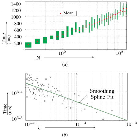
Figure 3: Convergence complexity: (a) illustrates little dependence of convergence on network size. (b) captures the $O(1/\epsilon)$ dependence

Proposition 7 (Properties)

The limiting GODDeS policy:

1. is loop-free

2. is the unique loop-free policy that disables the smallest set of transitions among all policies which induce the same measure vector for a given $\theta$.

Proof:

(1) Absence of loops follows immediately from noting that, in the limiting policy, a controllable transition $q_{i}\rightarrow q^{v}_{(ij)}$ is enabled if and only if $q^{v}_{(ij)}$ has a limiting measure strictly greater than that of $q_{i}$, implying that any sequence of transitions (with no consecutive repeating states) goes to either the dump or the sink in a finite number of steps.

(2) follows directly from the uniqueness and the maximal permissivity property of optimal policies computed by language measure-theoretic optimization (See [14]). ∎

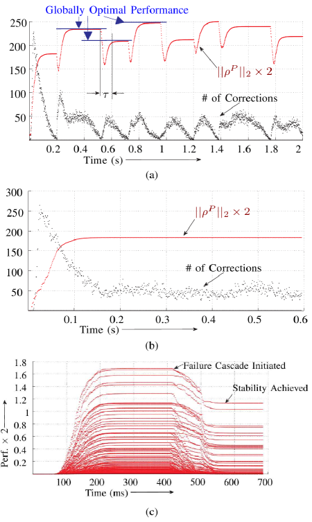
Figure 4: Convergence dynamics: (a) rapid convergence to large random sink movements (b)robust response to large zero-mean variations in the drop probabilities (c) response to failure cascade where $50\%$ of the nodes are killed

In this paper, we refrain from explicitly designing specific headers and data-structures that would be required for practical implementation of GODDeS. However one can easily tabulate the data that needs to be maintained at each node (See Table I). In particular, each node needs to know the unique network id. of each neighbor that it can communicate with (Col. 1), and their current measure values (Col. 3). The drop probabilities for communicating from self to each of those neighbors must be maintained as well, for the purpose of carrying out the GODDeS updates (Col. 4). The forwarding decision is a neighbor-specific Boolean value (Col. 5), which is set to $1$ if the neighbor currently has a strictly higher measure than self, and $0$ otherwise. The packets are then forwarded by randomly choosing (in an equiprobable manner) between the enabled neighbors, $i.e.$, the ones with a true forwarding decision. Note that this node data updates when the measures of the neighbors change (Col. 3), or the drop probabilities (Col. 4) update. However, changes in the measures may not necessarily reflect a change in the forwarding decisions. Also, note that the routing is inherently probabilistic, (due to the possibility that multiple enabled neighbors may exist for a given node). Furthermore, the optimal policy disables transmission to as few neighbors as possible for a specified $\theta$ (Proposition 7), and hence exploits multi-path transmissions in an optimal manner.

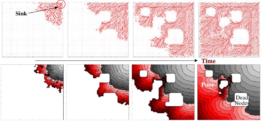
Figure 5: Convergence dynamics: Top plates illustrate the gradient of the scalar field induced by the measure values; bottom plates illustrate the level sets

In remote sensing applications nodes often have limited energy, necessitating route updates as high-traffic nodes get depleted. Also, local congestion arising due to the bursty nature of such communication may require re-routing. Note that congestion leads to higher packet drop probabilities, and gets reflected in the local link-specific drop probability estimations. Thus, GODDeS automatically corrects for network congestion to a large degree, by modulating the forwarding decisions as specific areas experience high traffic. However this does not correct for depleting energy levels (until the nodes actually die). Energy-aware reorganizations can be nevertheless carried out within the GODDeS framework autonomously and in a decentralized manner. Specifically, each node can regulate incoming traffic by deliberately reporting lower values of its current self-measure to its neighbors:

$$\textrm{\small\color[rgb]{.545,0,0}Reported}\longrightarrow r^{[k]}_{\theta}\big{|}_{i}=\zeta(q_{i},k)\nu^{[k]}_{\theta}\big{|}_{i}\leftarrow\textrm{\small\color[rgb]{0,.392,0}Computed}$$ (55)

where $\forall q_{i}\in Q,k\in[0,\infty),\zeta(q_{i},k)\in[0,1]$ is a multiplicative factor which is modulated to have decreasing values as node energy gets depleted, or as local congestion increases. Such modulation forces automatic self-organization to compute alternate routes that tend to avoid the particular node. The dynamics of such context-aware modulation may be non-trivial; while for slowly varying $\zeta(q_{i},k)$, the convergence results presented here is expected to hold true, rapid fluctuations in $\zeta(q_{i},k)$ may be problematic.

VI Verification, Validation & Discussion

Extensive simulations have been performed on NS2 network simulator, running on a 32 core (64 bit architecture) workstation with 128 GB of RAM. We investigate how convergence times scale as a function of the network size in Figures 3(a-b). $10^{2}$ random topologies were considered for each $N$ (increased from 25 to 1600), and the mean times along with the max-min bars are plotted in Figure 3(a). Note that the abscissa is on a logarithmic scale, and the near linear nature of the plot indicates a logarithmic dependence of the convergence on network size, implying that the bound computed in Proposition 6 is possibly not tight. The dependence on $\epsilon$ shown in Figure 3(b) (for $N=10^{3}$) is hyperbolic, as expected, leading to a near linear dependence after a smoothing spline fit on a log-log scale. Note the convergence times are not CPU times, but are estimated from NS2 output (using 802.11 standard).

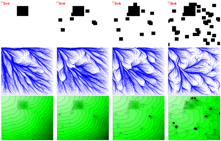
Figure 6: Time lapse plates for progressive node deaths: Top row indicates failed regions in black, middle row illustrates packet path signatures to the sink from operational nodes, and bottom row shows the level sets for the scalar field induced by the node measures

The theoretical convergence results are illustrated in Figure 4(a-c), which were generated on a $10^{4}$ node network. Plate (a) illustrates the variation of the number of route updates ($\#$ of forwarding decision corrections) and the norm of the performance vector $\rho^{P}$ (scaled up by a multiplicative factor of 2) when the sink is moved around randomly at a slower time scale. Since $\rho^{P}$ is the vector of end-to-end success probabilities (See Definition 14), its norm captures the degree of expected throughput across the network. Note that sink changes induce self-organizing corrections, which rapidly die down, with the performance converging close to the global optimal ($\epsilon=0.001$ was assumed in all the simulations). The drop probabilities are chosen randomly, and, on the average, held constant in the course of simulation illustrated in plate (a) (zero mean Gaussian noise is added to illustrate robustness). Note that the seemingly large fluctuations in the performance norm is unavoidable; the interval $\tau$ is the what it approximately takes for information to percolate through the network, and hence this much time is necessary at a minimum for decentralized route convergence. Plate (b) illustrates the effect of large zero-mean stochastic variations in the drop probabilities. Each node estimates the drop probabilities from simple windowed average of the link-specific packet drops. We note that large sustained fluctuations result in a sustained corrections in the forwarding decisions (which no longer goes to zero). However, the norm of the performance vector converges and holds steady, indicating a highly stable quality of service. This clearly illustrates that the information percolation strategy induces a low-pass filter eliminating high-frequency fluctuations, yielding a self-organizing routes that maintain high throughput in a robust manner. Note that small number of route fluctuations always occur (as shown by the non-zero number of corrections), but the key point is that this does not induce significant variations in the performance. Plate (c) illustrates the case where a cascading failure was simulated by turning off $50\%$ of the nodes in the network. We measure the individual entries of $\rho^{P}$ for a pre-determined set of nodes, which lie at a maximal distance from the sink (and are not killed). Note that the expected throughputs stabilize before the cascade, and the routes rapidly reorganize due to the failure event, when the performance regains convergent values. The entire process is perfectly decentralized, with the nodes identifying dead or non-responsive neighbors, and updating both their set of possible neighbors (Col. 2 in Table I), and self measures.

Convergence dynamics is explicitly illustrated in Figure 5, for a dense network of $10^{4}$ nodes, placed on an uniform rectangular grid (uniformity merely aids visualization). We see the gradual spreading out of the non-zero measure updates from the sink. The plates on top show the the gradient of the scalar field induced by the node measures, while those at the bottom illustrate the level sets. The voids are conglomerations of dead or non-responsive nodes. Other regions (marked “POOR”) comprise of nodes that are experiencing poor communication. Note that the routes tend to avoid these regions. As before, the drop probabilities are chosen randomly, and held constant on the average with zero mean Gaussian noise. Also, note the two color tones illustrate the possibility of simple decentralized thresholding, to autonomously segregate the network to classes which have a certain degree of connectivity to the sink, based on the convergent value of the estimated measures.

Progressive failures are simulated in Figure 6, addressing situations with gradual node depletions. Top row shows the failed regions in black. The network is initialized with $10^{4}$ nodes with energy levels distributed uniformly over a pre-specified range, leading to a realistic scenario, where nodes fail due to to various unmodeled effects in addition to energy spent in communication. Nodes are assumed to fail in clusters of $\sim 10^{2}$ creating dead regions. The middle row shows packet traces to the sink from operational nodes, and the bottom row illustrates the level sets. Note that with small number of dead regions, we can see very little “white” in the middle row, indicating high route utilization and low congestion. As the nodes fail, we see more white space, indicating that most packets are now taking similar routes. Note that congestion leads to higher drop probabilities which are estimated on the fly, and incorporated via GODDeS in local decision-making, thus implying significant congestion-awareness.

VII Conclusions & Future Work

This paper introduces GODDeS: a new routing algorithm designed to effectively exploit high quality paths in lossy ad-hoc wireless environments, typically with a large number of nodes. The routing problem is modeled as an optimal control problem for a decentralized Markov Decision Process, with links characterized by locally known packet drop probabilities that either remain constant on average or change slowly. The equivalence of this optimization problem to that of performance maximization of an explicitly constructed PFSA allows us to apply the theory of quantitative measures of probabilistic regular languages, and design a distributed highly efficient solution approach that attempts to minimize source-to-sink drop probabilities across the network. Theoretical results provide rigorous guarantees on global performance, showing that the algorithm achieves near-global optimality, in polynomial time. It is also argued that GODDeS is significantly congestion-aware, and exploits multi-path routes optimally. Theoretical development is supported by high-fidelity network simulation.

Future work will proceed in the following directions, primarily aimed at investigating and consequently relaxing some of the key assumptions made in this paper:

1. Design explicit strategies for energy and congestion awareness within the GODDeS framework. In particular, investigate the ramifications of various choices of the measure reduction factor described in Eq. (55).

2. Generalize the analysis to multiple sinks, which is not too difficult in view of the fact that most of the theoretical results carry over to the general case.

3. We assumed that the link-specific drop probabilities are estimated at the nodes. Grossly incorrect estimations will translate to incorrect routing decisions, and decentralized strategies for robust identification of these parameters need to be investigated at a greater depth.

4. Explicit design of implementation details such as packet headers, node data structures and pertinent neighbor-neighbor communication protocols.

5. Hardware validation with networks of different sizes, and with induced failure situations.

References

- [1] D. P. Bertsekas and R. G. Gallager, “Distributed asynchronous bellman-ford algorithm,” in Data Networks. Prentice Hall, Englewood Cliffs, 1987, ch. 5.2.4, pp. 325–333.
- [2] C. E. Perkins and E. M. Royer, “The ad hoc on-demand distance-vector protocol,” in Ad Hoc Networking, C. E. Perkins, Ed. Addison-Wesley, 2001, ch. 6, pp. 173–219.
- [3] ——, “Ad-hoc on-demand distance vector routing,” in 2nd IEEE Workshop on Mobile Computing Systems and Applications, New Orleans, USA. IEEE, February 1999, pp. 90–100.
- [4] D. B. Johnson, D. A. Maltz, and J. Broch, “Dsr: The dynamic source routing protocol for multihop wireless ad hoc networks,” in Ad Hoc Networking, C. Perkins, Ed. Addison-Wesley, 2001, pp. 139–172.
- [5] A. Pandey, M. N. Ahmed, N. Kumar, and P. Gupta, “A hybrid routing scheme for mobile ad hoc networks with mobile backbones,” in International Conference on High Performance Computing, IEEE. IEEE, December 2006, pp. 411–423.
- [6] G. Koltsidas, G. Dimitriadis, and F.-N. Pavlidou, “On the performance of the hsls routing protocol for mobile ad hoc networks,” Wirel. Pers. Commun., vol. 35, no. 3, pp. 241–253, 2005.
- [7] P. Jacquet, P. Mühlethaler, T. Clausen, A. Laouiti, A. Qayyum, and L. Viennot, “Optimized link state routing protocol,” in IEEE INMIC’01, Lahore, Pakistan, IEEE. IEEE, December 2001, pp. 62–68.
- [8] M. JoaNg and I. Lu, “A peer-to-peer zone-based two-level link state routing for mobile ad hoc networks,” IEEE Journal on Selected Areas In Communication, vol. 17, no. 8, pp. 1415–1425, August 1999.
- [9] C. Intanagonwiwat, R. Govindan, and D. Estrin, “Directed diffusion: A scalable and robust communication paradigm for sensor networks,” in Proceedings of the 6th annual international conference on Mobile. New York, USA: ACM Press, 2000, pp. 56–67.
- [10] D. S. J. D. Couto, D. Aguayo, J. Bicket, and R. Morris, “A high-throughput path metric for multi-hop wireless routing,” Wireless Networks, vol. 11, pp. 419–434, 2005.
- [11] B. Awerbuch, D. Holmer, and H. Rubens, “High throughput route selection in multi-rate ad hoc wireless networks,” in WONS, 2004, pp. 253–270.
- [12] D. S. Bernstein, R. Givan, N. Immerman, and S. Zilberstein, “The complexity of decentralized control of markov decision processes,” in Proceedings of the Sixteenth Conference on Uncertainty in Artificial Intelligence (UAI-2000), 2000, pp. 32–37.
- [13] ——, “The complexity of decentralized control of markov decision processes,” Math. Oper. Res., vol. 27, no. 4, pp. 819–840, 2002.
- [14] I. Chattopadhyay and A. Ray, “Language-measure-theoretic optimal control of probabilistic finite-state systems,” International Journal of Control, vol. 80, no. 8, pp. 1271–1290, Aug. 2007.
- [15] J. E. Hopcroft, R. Motwani, and J. D. Ullman, Introduction to Automata Theory, Languages, and Computation, 2nd ed. Addison-Wesley, 2001.
- [16] R. Bapat and T. Raghavan, Nonnegative matrices and Applications. Cambridge University Press, 1997.
- [17] W. Rudin, Real and Complex Analysis, 3rd ed. McGraw Hill, New York, 1988.
- [18] I. Chattopadhyay and A. Ray, “Optimal control of infinite horizon partially observable decision processes modeled as generators of probabilistic regular languages,” International Journal of Control, vol. 83, no. 3, pp. 457–483, March 2010.
- [19] S. Gerschgorin, “Über die abgrenzung der eigenwerte einer matrix,” Izv. Akad. Nauk. USSR Otd. Fiz.-Mat. Nauk, vol. 7, pp. 749–754, 1931.
- [20] R. S. Varga, Gerschgorin and His Circles. Germany: Springer, 2004.