THE OPTX PROJECT IV: How Reliable is [OIII] as a Measure of AGN Activity?

Abstract

We compare optical and hard X-ray identifications of active galactic nuclei (AGNs) using a uniformly selected (above a flux limit of $f_{\rm 2-8~{}keV}=3.5\times 10^{-15}$ erg cm^-2 s^-1) and highly optically spectroscopically complete ($>80$% for $f_{\rm 2-8~{}keV}>10^{-14}$ erg cm^-2 s^-1 and $>60$% below) $2-8$ keV sample observed in three Chandra fields (CLANS, CLASXS, and the CDF-N). We find that empirical emission-line ratio diagnostic diagrams misidentify $20-50$% of the X-ray selected AGNs that can be put on these diagrams as star formers, depending on which division is used. We confirm that there is a large (2 orders in magnitude) dispersion in the log ratio of the [OIII]$\lambda 5007$ (hereafter, [OIII]) to hard X-ray luminosities for the non-broad line AGNs, even after applying reddening corrections to the [OIII] luminosities. We find that the dispersion is similar for the broad-line AGNs, where there is not expected to be much X-ray absorption from an obscuring torus around the AGN nor much obscuration from the galaxy along the line-of-sight if the AGN is aligned with the galaxy. We postulate that the X-ray selected AGNs that are misidentified by the diagnostic diagrams have low [OIII] luminosities due to the complexity of the structure of the narrow-line region, which causes many ionizing photons from the AGN not to be absorbed. This would mean that the [OIII] luminosity can only be used to predict the X-ray luminosity to within a factor of $\sim 3$ (one sigma). Despite selection effects, we show that the shapes and normalizations of the [OIII] and transformed hard X-ray luminosity functions show reasonable agreement, suggesting that the [OIII] samples are not finding substantially more AGNs at low redshifts than hard X-ray samples.

1. Introduction

Determining which sources in a large sample of galaxies host active galactic nuclei (AGNs) at their centers is a challenging but essential step for galaxy evolution studies. The most common method used optically to separate star-forming galaxies from AGNs is a Baldwin et al. (1981)-type empirical diagnostic diagram (hereafter, BPT diagram; see also Osterbrock & Pogge 1985 and Veilleux & Osterbrock 1987) of the narrow emission-line ratios [OIII]$\lambda 5007$/H$\beta$ versus [NII]$\lambda 6584$/H$\alpha$. In this diagram galaxies occupy two well-defined wings: the left wing consists of star-forming galaxies, while the right wing is attributed to galaxies with an active nucleus (e.g., Kauffmann et al., 2003; Stasińska et al., 2006; Kewley et al., 2006). The basic idea underlying these diagrams is that the emission lines in star-forming galaxies are powered by massive stars, so there is a well-defined upper limit on the intensities of the collisionally excited lines relative to the recombination lines (such as H$\alpha$ or H$\beta$). In contrast, AGNs are powered by a source of far more energetic photons, making the collisionally excited lines more intense relative to the recombination lines.

Kauffmann et al. (2003) and Heckman et al. (2004) proposed using the luminosity of the [OIII]$\lambda 5007$ (hereafter, [OIII]) line as a tracer of AGN activity. As they pointed out, the advantages of the [OIII] line are that (1) it is typically strong and easy to detect; and (2) although it can be excited by both massive stars and AGNs, it has been observed to be relatively weak in metal-rich, star-forming galaxies. However, the disadvantage is that one needs to assume that [OIII] is an unbiased, orientation-independent indicator of the ionizing flux from the AGN.

In the standard ‘unified’ model for AGNs (e.g., Antonucci, 1993), if the observer’s view of a galaxy’s central supermassive black hole and its associated continuum and broad emission-line region are unobscured (obscured) by the presence of a dusty torus, then it is a type 1 (type 2) AGN. However, even in the type 2 AGNs the covering factor is not one, so radiation is able to escape through the opening angle and photoionize the gas located several hundred parsecs or more from the central engine. This gives rise to the narrow emission-line region with its strong narrow permitted and forbidden emission lines. Since the narrow emission-line region lies outside of the dusty torus, the emission lines should not suffer from obscuration by that high column density material (though they may be affected by dust within the host galaxy). Although there is some evidence that the [OIII] luminosity is a good measure of AGN activity (e.g., Mulchaey et al., 1994), and, indeed, many researchers have assumed it to be so in their analyses (e.g., Alonso-Herrero et al., 1997; Hao et al., 2005; Netzer et al., 2006; Bongiorno et al., 2010), recent work has called this conclusion into question (e.g., Cocchia et al., 2007; Meléndez et al., 2008; Diamond-Stanic et al., 2009; La Massa et al., 2009).

With the advent of the Chandra and XMM-Newton X-ray observatories, AGN activity can now also be traced through the $2-10$ keV luminosity, although this measurement may suffer from some absorption (e.g., Diamond-Stanic et al., 2009; La Massa et al., 2009). Also, X-ray selection misses the most heavily absorbed, Compton-thick sources with $N_{H}>10^{24}$ cm^-2 (see Comastri 2004 for a review). An interesting question is how well the X-ray and optical selections compare. With our large, uniform, and highly optically spectroscopically complete OPTX sample of X-ray selected AGNs, we are in a good position to do this comparison. The OPTX sample consists of one deep pencil-beam survey (Chandra Deep Field-North or CDF-N) and two moderately deep wide-field surveys (Chandra Large Area Synoptic X-ray Survey or CLASXS and Chandra Lockman Area North Survey or CLANS).

In this paper we explore how well the BPT diagram does at classifying as AGNs the sources in the OPTX X-ray selected AGN sample and how that classification relates to the very broad observed range in $L_{2-10~{}{\rm keV}}/$$L_{\rm[OIII]}$ (e.g., Cocchia et al., 2007; Meléndez et al., 2008; La Massa et al., 2009). Following Heckman et al. (2005), Bongiorno et al. (2010), and Georgantopoulos & Akylas (2010), we use our measurements of the mean luminosity ratios to transform the fits to the OPTX+SWIFT BAT hard X-ray luminosity function (LF) from Yencho et al. (2009) and the local RXTE hard X-ray LF from Sazonov & Revnivtsev (2004) into [OIII] LFs, which we then compare with the SDSS [OIII] LFs from Hao et al. (2005) and Reyes et al. (2008) to investigate the efficiency of optical versus X-ray selection.

The structure of the paper is as follows. In Section 2 we briefly describe our $2-8$ keV Chandra selected OPTX sample. In Section 3 we determine optical narrow emission-line luminosities and investigate the effects of line reddening. In Section 4 we test how many X-ray selected AGNs are misidentified as star formers by the BPT diagram. In Section 5 we plot the ratio of the [OIII] luminosities to the $2-8$ keV luminosities versus the $2-8$ keV luminosities for our non-BLAGNs and look for any luminosity dependence, as suggested by Netzer et al. (2006). In Section 6 we discuss the probable impact of the observed dispersion in this luminosity ratio on the BPT classification of X-ray AGNs. We then align various hard X-ray and [OIII] LFs for comparison. In Section 7 we summarize our results and their implications.

All magnitudes are in the AB magnitude system, and we assume $\Omega_{M}=0.3,\Omega_{\Lambda}=0.7$, and H${}_{0}=70$ km s^-1 Mpc^-1.

2. Sample

In Trouille et al. (2008) we presented the X-ray catalog for the CLANS field. We also presented the optical and infrared photometry and the spectroscopic and photometric redshifts for the X-ray sources in all three of the OPTX fields (CLANS, CLASXS, and CDF-N). In Trouille et al. (2009) we updated the X-ray catalog for the CLANS field, including 28 sources that had inadvertently been dropped in the original catalog, and we provided additional spectroscopic redshifts for this field.

In Trouille et al. (2009) we used a uniform and highly significant subsample of the OPTX sources to compare the optical spectral types with the X-ray spectral properties. Here we use the same selection of sources in the $2-8~{}\rm keV$ band with significance greater than $3~{}\sigma$ and fluxes greater than the flux limits (for a $S/N=3$) at the pointing center of the $70$ ks CLANS pointings. There are 746 X-ray sources in this $2-8~{}\rm keV$ sample (410, 251, and 85 sources from the CLANS, CLASXS, and CDF-N fields, respectively). Our optical spectroscopic completeness with the DEep Imaging Multi-Object Spectrograph (DEIMOS; Faber et al. 2003) on the Keck II 10 m telescope is very high (see Table 3 of Trouille et al. 2009), particularly at the bright flux end. At $f_{2-8~{}\rm keV}>1.4\times 10^{-14}$ erg cm^-2 s^-1 (the break flux in the $2-8~{}\rm keV$ number counts; see Trouille et al. 2008) we have spectroscopic redshifts for 178 of the 217 sources (i.e., we are 82% complete to this flux).

In Trouille et al. (2009) we followed Szokoly et al. (2004) and Barger et al. (2005) and classified the spectroscopically identified sources into four optical spectral types: absorbers (ABS; no strong emission lines); (2) star formers (SF; strong Balmer lines and no broad or high-ionization lines); (3) high-excitation sources (HEX; [NeV], CIV, narrow MgII lines, or strong [OIII]); and (4) broad-line AGNs (BLAGNs; optical lines having FWHM line widths $>2000$ km s^–1). Although the HEX spectral type largely overlaps the classical Seyfert 2 spectral type, describing the sources as HEX sources helps to avoid confusion with the classical definitions.

In Trouille et al. (2008, 2009) we used the X-ray fluxes and spectroscopic plus photometric redshifts to calculate the rest-frame $2-8~{}\rm keV$ luminosities, $L_{X}$. At $z<3$ (which is all we will be considering in this paper), we calculated the luminosities from the observed-frame $2-8~{}\rm keV$ fluxes, assuming an intrinsic $\Gamma=1.8$. That is, $L_{X}=f\times 4\pi d_{L}^{2}\times K-$ correction, where for $z<3$

$$K-\textrm{corr}=(1+z)^{-0.2}~{}\textrm{and}~{}f=f_{2-8~{}\rm keV}\,.$$ (1)

Note that using the individual photon indices (rather than the universal power-law index of $\Gamma=1.8$ adopted here) to calculate the $K-$ corrections would result in only a small difference in the rest-frame luminosities (Barger et al., 2002). We have not corrected the X-ray luminosities for absorption. We will examine the impact of this approach in Section 6.

Any source more luminous than $L_{X}=10^{42}$ erg s^-1 is very likely to be an AGN on energetic grounds (Zezas et al., 1998; Moran et al., 1999). Of the 746 sources in our $2-8~{}\rm keV$ sample, 619 have $L_{X}>10^{42}$ erg s^-1. If we adopt the Ranalli et al. (2003) relation between star-formation rate (SFR) and X-ray luminosity

$$L_{2-10~{}\rm keV}=\textrm{SFR}/M_{\sun}\times 5\times 10^{39}~{}\textrm{erg s}^{-1},$$ (2)

we find that a SFR of at least 200 $M_{\sun}$ yr^-1 is required to produce an X-ray luminosity greater than $10^{42}$ erg s^-1. Given that the space density of ultraluminous infrared galaxies (ULIRGs, which require a SFR $>200~{}M_{\sun}$) is approximately $10^{-5}$ Mpc^-3 at $z\sim 0.9$ (Magnelli et al., 2009), near the peak in our redshift distribution, and our OPTX fields cover $\sim 1.2$ deg², we expect $\sim 30$ ULIRGs total in our sample. Because the space density of ULIRGs increases rapidly with redshift, if instead we restrict our analysis to $z<0.5$ (see Section 4), we expect fewer than three ULIRGs contaminating our sample. Since the contamination rate is low ($\sim 5$% of our sample), we assume that the 619 $L_{X}>10^{42}$ erg s^-1 sources are AGNs (although see Section 4 for our classifications of these sources as star formation or AGN dominated using emission-line ratio diagnostics). In the remainder of this work, our ‘$2-8~{}\rm keV$ sample’ refers to these 619 sources.

3. High-Ionization Narrow Emission Lines

3.1. ${\rm[OIII]}\lambda 5007$

[OIII] appears in our optical spectra for sources with $z<0.95$. Since DEIMOS degrades at the red end, we limit our [OIII] analysis to the 157 sources in our $2-8~{}\rm keV$ sample with spectroscopic redshifts less than $0.85$. We use the method described in Kakazu et al. (2007) to determine the [OIII] flux. We first determine which bandpass covers the redshifted emission line. We then integrate the spectrum convolved with that bandpass filter response and set the result equal to the broadband flux to determine the normalization factor. We determine the continuum using a sliding 250 Å median. We then multiply the integrated continuum-subtracted emission line by the normalization factor to obtain the flux in the line. This procedure only works for sources with secure continuum magnitudes where the sky subtraction can be well determined in the spectra. We then convert the emission-line flux into an emission-line luminosity using $L_{\rm[OIII]}$ $=f_{\rm[OIII]}\times 4\pi d_{L}^{2}$.

In Figure 1 we show rest-frame $2-8~{}\rm keV$ luminosity versus redshift for the sources in our $2-8~{}\rm keV$ sample for which we were able to determine $L_{\rm[OIII]}$ (black symbols; 122 of the 157 sources). We denote non-BLAGNs by triangles and BLAGNs by squares. Of the 35 sources that are lacking $L_{\rm[OIII]}$ determinations, 22 are classified as absorbers (magenta circles). By definition, absorbers exhibit little to no strength in emission lines. However, they do exhibit H$\beta$ absorption (and H$\alpha$ as well for those with a low enough redshift). The presence of these Balmer absorption lines suggests that they are not BL Lac objects (see Laurent-Muehleisen et al. 1998 for a detailed description of BL Lac properties). We note that if these are in fact low luminosity BL Lac objects, their low non-thermal optical luminosity could allow for the presence of stellar absorption lines. We use an equivalent width for the [OIII] line that is $1\sigma$ above the noise to determine the upper limit on $L_{\rm[OIII]}$ for these sources.

The remaining 13 sources lack $L_{\rm[OIII]}$ determinations as a result of observational complications. Six sources (red symbols) are fainter than the limiting magnitude in the filter needed to determine their $L_{\rm[OIII]}$ values. Four sources (green symbols) have sky lines that interfere with the $L_{\rm[OIII]}$ determinations, and three sources (blue symbols) have an intervening absorption line located at the position of [OIII]. We remove these 13 sources from our subsequent analysis.

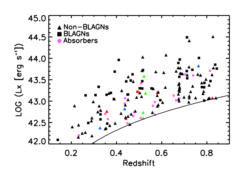
Figure 1.— Log$(L_{X})$ vs. redshift for sources in our $2-8~{}\rm keV$ sample (black—sources with $L_{\rm[OIII]}$ determinations; magenta—absorbers; red—sources lacking magnitudes in the necessary filter; green—sources with sky line interference; blue—sources with intervening absorption interference). Non-BLAGNs are denoted by triangles, BLAGNs by squares, and absorbers by circles, as noted in the legend. The black curve corresponds to the flux limit for our $2-8~{}\rm keV$ sample.

3.2. Emission-Line Reddening

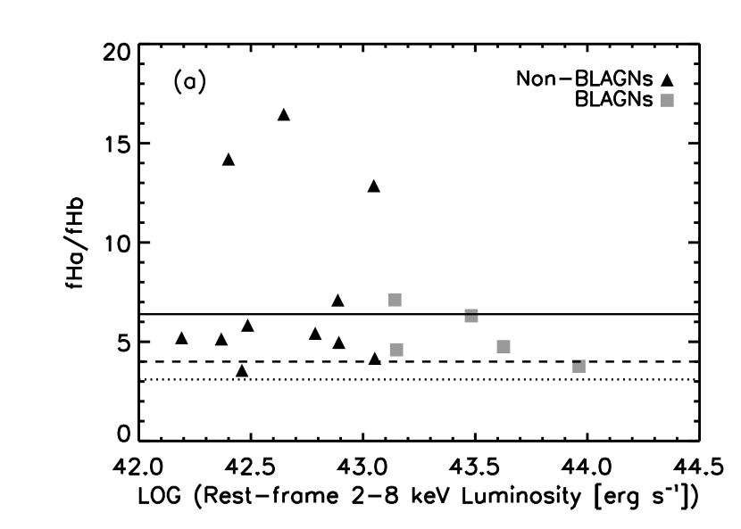
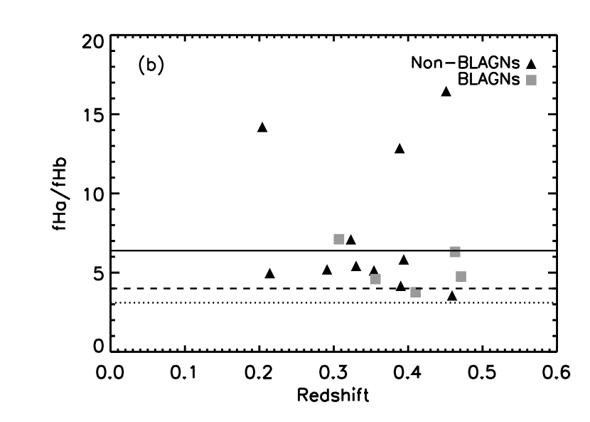
Figure 2.— (a) Ratio of H$\alpha$ flux to H$\beta$ flux vs. rest-frame $2-8~{}\rm keV$ luminosity for sources in our $2-8~{}\rm keV$ sample with reliable $f_{\rm{H}\alpha}$ and $f_{\rm{H}\beta}$ measurements (dotted line—the canonical intrinsic Balmer decrement ($f_{\rm{H}\alpha}/f_{\rm{H}\beta}$$)_{o}=3.1$; dashed line—the Zakamska et al. (2003) reddening value for their composite SDSS type 2 AGN spectrum, $f_{\rm{H}\alpha}/f_{\rm{H}\beta}$ $=4.0$; solid line—the Bassani et al. (1999) median reddening value for their sample of type 2 AGNs, $f_{\rm{H}\alpha}/f_{\rm{H}\beta}$ $=6.4$. (b) Same as (a) but versus redshift.

The average reddening towards the narrow-line region in AGNs is still a matter of debate. Studies using HST spectroscopy combined with the IUE-based analysis of Ferland & Osterbrock (1986) suggest that the narrow emission-line reddening for non-BLAGNs corresponds to $E(B-V)=0.2-0.4$ mag (e.g., Ferruit et al., 1999). Zakamska et al. (2003) used the Balmer decrement, $f_{\rm{H}\alpha}/f_{\rm{H}\beta}$, measured from a composite spectrum of their SDSS non-BLAGNs as a proxy for the volume averaged narrow emission-line reddening and found a similar result of $E(B-V)=0.27$ mag (though see Netzer et al. 2006 for a discussion of possible selection effects). Dahari & De Robertis (1988) and Bassani et al. (1999) found significantly larger median reddening in their non-BLAGNs of $E(B-V)=0.48$ mag and $E(B-V)=0.65$ mag, respectively. The Dahari & De Robertis (1988) sample represented the largest available uniform database of optical spectra at that time, including most of the known Markarian Seyferts and a majority of the classical Seyferts listed in Weedman (1977, 1978). The median reddening quoted above is for the 20 Seyfert 1s in their sample with $z<0.03$ and axial ratios $b/a>0.5$. The Bassani et al. (1999) sample was composed of the 57 Seyfert 2s with reliable hard X-ray spectra in the literature at that time. They obtained the Balmer decrements from a variety of sources. The majority of their sources have $z<0.06$, with a few at $z<0.2$.

In Figure 2 we show $f_{\rm{H}\alpha}/f_{\rm{H}\beta}$ versus (a) rest-frame $2-8~{}\rm keV$ luminosity and (b) redshift for the 16 sources in our $2-8~{}\rm keV$ sample for which we were able to measure both the H$\alpha$ and H$\beta$ fluxes. For reference, there are 45 non-BLAGNs and 19 BLAGNs with $0<z\leq 0.5$ (the redshift at which H$\alpha$ leaves our spectral window) in our $2-8~{}\rm keV$ sample. The separation between BLAGNs (gray squares) and non-BLAGNs (black triangles) with luminosity is a result of BLAGNs dominating the number densities at higher X-ray luminosities (Steffen et al., 2003; Ueda et al., 2003; Barger et al., 2005; La Franca et al., 2005; Simpson, 2005; Akylas et al., 2006; Beckmann et al., 2006; Sazonov et al., 2007; Hasinger, 2008; Silverman et al., 2008; Winter et al., 2009; Yencho et al., 2009). This result had previously been noted in the radio by Lawrence & Elvis (1982).

To determine the H$\alpha$ and H$\beta$ fluxes for the non-BLAGNs we use the same procedure as described in Section 3.1 for determining the [OIII] emission-line fluxes. However, to properly account for stellar Balmer absorption, we first fit a stellar population model to the continuum using the Tremonti et al. special-purpose template fitting code (private communication), described in detail in Tremonti et al. (2004). In brief, we use a grid of stellar template models covering a range of age and metallicity generated by the Bruzual & Charlot (2003) population synthesis code. For each galaxy we transform the templates to the appropriate redshift and velocity dispersion to match the data. We then subtract the best-fit model from the continuum. We only do the subtraction in our determination of the H$\beta$ emission-line flux, because the H$\alpha$ line is typically stronger with a relatively weaker underlying stellar absorption. We find an average equivalent width of $\sim 1$ Å for the H$\beta$ stellar absorption. This is in agreement with the fixed offset of $1$ Å used in Cowie & Barger (2008), which they determined from their averaged absorption-line galaxy spectrum.

To determine the H$\alpha$ and H$\beta$ fluxes for the BLAGNs, we fit both a broad and a narrow component to the lines, subtract the broad component, and then follow the same procedure as described above. We are able to determine reliably the H$\alpha$ and H$\beta$ fluxes for 26% (22%) of the BLAGNs (non-BLAGNs) in our $2-8~{}\rm keV$ sample with $0<z\leq 0.5$.

We do not see any statistically significant difference in the reddening between our BLAGNs and our non-BLAGNs, nor do we see a dependence on redshift or X-ray luminosity. We note the small numbers in our sample and the three non-BLAGNs with significantly higher $f_{\rm{H}\alpha}/f_{\rm{H}\beta}$ values. The average $f_{\rm{H}\alpha}/f_{\rm{H}\beta}$ for the combined samples is $5.2\pm 3.1$ (corresponding to $E(B-V)=0.47\pm 0.4$), which falls between the Zakamska et al. (2003, dashed line) and Bassani et al. (1999, solid line) results. The dotted line shows the canonical intrinsic Balmer decrement value, ($f_{\rm{H}\alpha}/f_{\rm{H}\beta}$$)_{o}=3.1$ (Ferland & Netzer, 1983; Osterbrock & Martel, 1993).

Following Bassani et al. (1999), we correct our narrow emission line fluxes for optical reddening with the equation

$$f_{\rm[OIII],\,corr}=f_{\rm[OIII]}\times[(f_{\rm{H}\alpha}/f_{\rm{H}\beta})/(f_{\rm{H}\alpha}/f_{\rm{H}\beta})_{o}]^{2.94}\,.$$ (3)

We use our calculated $f_{\rm{H}\alpha}/f_{\rm{H}\beta}$ values for the 16 sources in which both lines are measured and the average $f_{\rm{H}\alpha}/f_{\rm{H}\beta}$= 5.2 for the remaining sources. This results in an average ratio between our extinction-corrected and non-extinction-corrected luminosities of 4.6. However, we caution that there remain many uncertainties when applying standard extinction corrections to AGN emission-line luminosities. For example, Hao et al. (2005) argue that AGNs may have higher intrinsic $f_{\rm{H}\alpha}/f_{\rm{H}\beta}$ ratios than normal galaxies because of higher densities and radiative transfer effects. Also, the relative distribution of dust and emission-line gas does not necessarily follow the simple model in which dust forms a homogeneous screen in front of the line-emitting regions.

A Kolmogorov-Smirnov (K-S) test reveals no significant difference in the distributions of $L_{\rm[OIII]}$ for our $z\leq 0.5$ BLAGNs and non-BLAGNs ($p=0.5$). We do not include the upper limit values for our absorbers in this comparison. This is in contrast with Diamond-Stanic et al. (2009), who find a statistically significant difference in the $L_{\rm[OIII]}$ distributions of their optically-selected Revised Shapley-Ames sample of Seyfert 1s and Seyfert 2s.

4. Emission-Line Ratio Diagnostic Diagrams

BPT emission-line ratio diagnostic diagrams can be used to infer whether the gas in a galaxy is primarily being heated by star formation or by radiation from an accretion disk around a central supermassive black hole. As discussed in Section 1, sources whose signal is dominated by accretion lie to the upper-right of those dominated by star formation. BPT diagrams are typically only applied to narrow-line active galaxies, because in BLAGNs the narrow lines are overwhelmed by emission from the broad-line region.

In Figure 3 we plot $\log($[OIII]/H$\beta)$ versus $\log($[NII]/H$\alpha)$ for the 21 sources in our $2-8~{}\rm keV$ sample for which we were able to determine the equivalent widths of all four emission lines (note that all 21 have $L_{X}>10^{42}$ erg s^-1). Of the seven $z\leq 0.5$ non-BLAGNs with $L_{X}>10^{43}$ erg s^-1 and measured [OIII] luminosities, only two appear in Figure 3. We note that this is a result of observational complications—sky lines interfering with our measurement of the H$\beta$, H$\alpha$, or [NII] lines or because the H$\alpha$/[NII] lines lie within the noise at the red edge of our spectral window.

The symbols grow in size and change in color with increasing X-ray luminosity. The dotted curve traces the Kewley et al. (2001) division between AGNs and extreme starbursts. It is a theoretical curve based on photoionization models for giant HII regions and a range of stellar population synthesis codes. The dashed curve traces the Kauffmann et al. (2003) division between AGN and star formers, which is based on an empirical separation of SDSS galaxies.

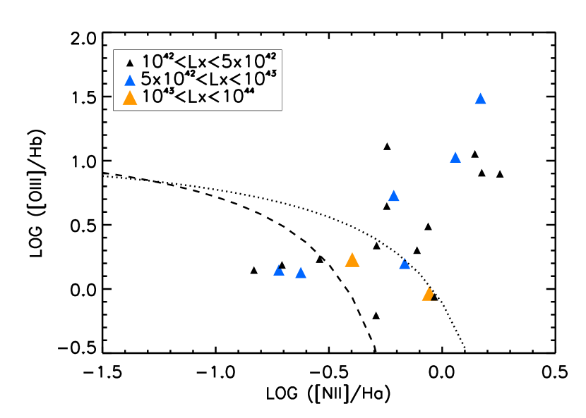
Figure 3.— (a) A BPT diagram for the non-BLAGNs in our $2-8~{}\rm keV$ sample with $z\leq 0.5$. The symbols grow in size and change in color with increasing X-ray luminosity, as indicated in the legend. The dashed curve denotes the Kauffmann et al. (2003) division between AGNs (upper-right) and star forming galaxies (lower-left). The dotted curve denotes the Kewley et al. (2001) division between AGNs and extreme starbursts.

Less than half ($10/21$) of the X-ray selected sources lie to the upper-right of the Kewley et al. (2001) curve and form a sequence similar to that of the SDSS Seyfert 2s, emerging from the HII region sequence and extending to the upper right-hand side of the diagram. Hereafter, we refer to these sources as ‘BPT AGN-dominated non-BLAGNs’. We also refer to the sources that lie to the lower-left of the Kauffmann et al. (2003) division as ‘BPT SF-dominated non-BLAGNs’ and those that lie between the two curves as ‘BPT transition non-BLAGNs’. We note that of the three BPT SF-dominated non-BLAGNs with $10^{42}<L_{X}<5\times 10^{42}$ erg s^-1 (black triangles), none have $L_{X}<2.5\times 10^{42}$ erg s^-1. A SFR of $>500~{}M_{\sun}$ is required to produce this level of X-ray luminosity (see Equation 2). Based on the space density of such strongly starbursting sources, we do not expect any in our $z<0.5$ $2-8~{}\rm keV$ sample.

Since two $L_{X}>10^{43}$ erg s^-1 AGN lie in the transition region and two $5\times 10^{42}<L_{X}<10^{43}$ erg s^-1 AGNs lie below the Kauffmann et al. (2003) line, it is clear that the optical diagnostic diagram is not able to classify all of the X-ray selected non-BLAGNs with line ratio measurements as AGNs. Given that we are working from a high X-ray luminosity sample, this seems rather surprising. However, since it has been shown by many authors that there is considerable spread in $L_{\rm[OIII]}/L_{X}$ (e.g., Alonso-Herrero et al., 1997; Bassani et al., 1999; Guainazzi et al., 2005; Heckman et al., 2005; Ptak et al., 2006; Netzer et al., 2006; Cocchia et al., 2007; Meléndez et al., 2008; Diamond-Stanic et al., 2009; La Massa et al., 2009), it is worth exploring whether this might affect how much overlap there is between the two AGN selections.

Figure 4.— (a) Histogram of the $\log(L_{\rm[OIII]}/L_{X})$ for the sources in our $2-8~{}\rm keV$ sample (solid line—$z\leq 0.85$ BLAGNs; dashed line—$z\leq 0.5$ BPT AGN-dominated non-BLAGNs). The arrow marks the mean value of the Heckman et al. (2005) extinction-uncorrected [OIII]-bright optically selected sample of Seyfert 1s. (b) Same as (a) but for $\log(L_{\rm[OIII],\,corr}/L_{X})$. The arrow marks the mean value of the Mulchaey et al. (1994) extinction-corrected optically selected sample of Seyfert 1s.

5. The Relation Between $L_{\rm[OIII]}$ and $L_{X}$

In Figure 4 we show the distribution of (a) $\log(L_{\rm[OIII]}/L_{X})$ and (b) $\log(L_{\rm[OIII],\,corr}/L_{X})$ for the BPT AGN-dominated non-BLAGNs (dashed line). They cover two orders in magnitude, confirming previous results that showed a very large spread in this ratio. We also show the distribution for the $z\leq 0.85$ BLAGNs (solid line).

In Table 1 we give the mean and standard deviation in $\log(L_{\rm[OIII]}/L_{X})$ and $\log(L_{\rm[OIII],\,corr}/L_{X})$ for the $z\leq 0.5$ BPT AGN-dominated non-BLAGNs, for the $z\leq 0.5$ and $z\leq 0.85$ non-BLAGNs, and for the $z\leq 0.5$ and $z\leq 0.85$ BLAGNs. In determining the mean values for the $z\leq 0.5$ and $z\leq 0.85$ non-BLAGNs, we do not include the upper limit values for the absorbers (see Section 3.1). We find that the mean values for the $z\leq 0.85$ BLAGNs agree with those from the optically selected Heckman et al. (2005) extinction-uncorrected and Mulchaey et al. (1994) extinction-corrected Seyfert 1 samples (as indicated by the arrows in Figure 4).

Table 1$\log(L_{\rm[OIII]}/L_{X})$

	Mean	($\sigma$)
BPT AGN-dom non-BLAGNs ($z\leq 0.5$)	-1.06 (-0.36)	0.6 (0.6)
Non-BLAGNs ($z\leq 0.5$)	-1.46 (-0.72)	0.6 (0.7)
Non-BLAGNs ($z\leq 0.85$)	-1.66 (-0.97)	0.5 (0.6)
BLAGNs ($z\leq 0.5$)	-1.85 (-1.27)	0.5 (0.8)
BLAGNs ($z\leq 0.85$)	-1.76 (-1.14)	0.5 (0.7)

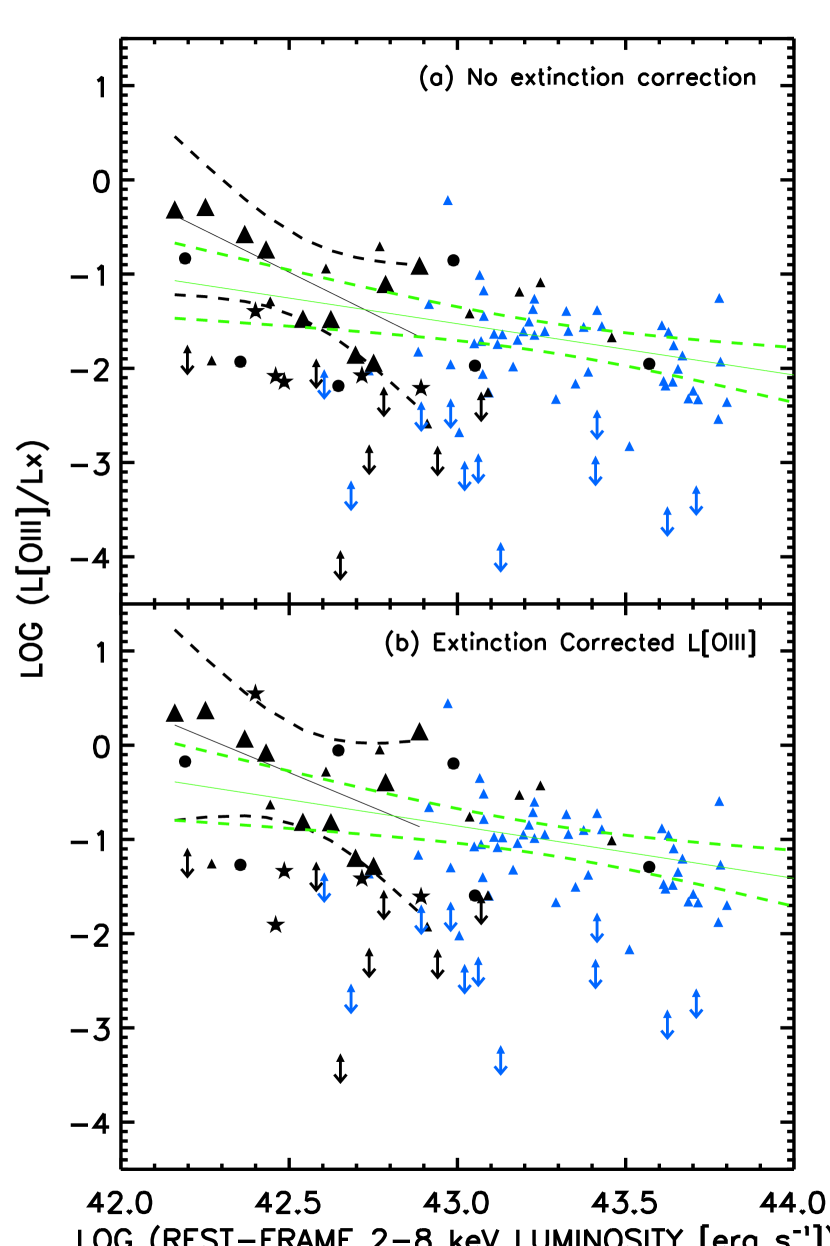
Figure 5.— (a) $\log(L_{\rm[OIII]}/L_{X})$ vs. $\log$ $L_{X}$ for the $L_{X}>10^{42}$ erg s^-1 non-BLAGNs in our $2-8~{}\rm keV$ sample (black small triangles—$z\leq 0.5$ non-BLAGNs lacking BPT line ratio measurements (excluding absorbers); black large triangles—$z\leq 0.5$ BPT AGN-dominated non-BLAGNs; stars—$z\leq 0.5$ BPT SF-dominated non-BLAGNs; circles—$z\leq 0.5$ BPT transition non-BLAGNs; blue small triangles—$0.5<z\leq 085$ non-BLAGNs). The upper limits indicate the absorbers in our $2-8~{}\rm keV$ sample (see Section 3). The $L_{\rm[OIII]}$ values are not extinction-corrected. The black (green) solid line shows the linear best fit to the $z\leq 0.5$ BPT AGN-dominated non-BLAGNs (the $z\leq 0.5$ BPT AGN-dominated sources plus the $0.5<z\leq 0.85$ non-BLAGNs). The dashed curves show the 95% confidence intervals. We do not include the absorber upper limit values in our best fit. (b) Same as (a) but for $L_{\rm[OIII]}$ extinction-corrected values.

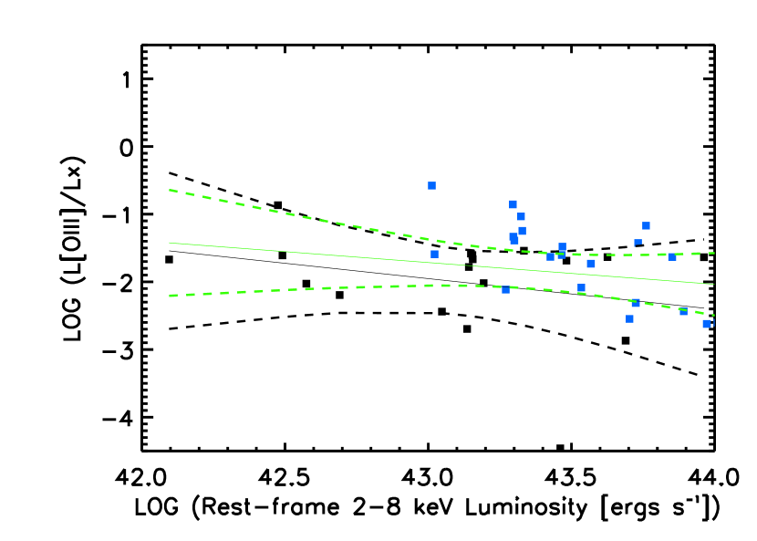
Figure 6.— $\log(L_{\rm[OIII]}/L_{X})$ vs. $\log$ $L_{X}$ for the $L_{X}>10^{42}$ erg s^-1 BLAGNs with $z\leq 0.5$ (black squares) and $0.5<z\leq 0.85$ (blue squares) in our $2-8~{}\rm keV$ sample. The $L_{\rm[OIII]}$ values are not extinction-corrected. The black (green) solid line shows the linear best fit to the $z\leq 0.5$ ($z\leq 0.85$) BLAGNs. The dashed curves show the 95% confidence intervals.

In Figure 5 we plot (a) $\log(L_{\rm[OIII]}/L_{X})$ versus $\log$ $L_{X}$ and (b) $\log(L_{\rm[OIII],\,corr}/L_{X})$ versus $\log$ $L_{X}$ for the non-BLAGNs in our $2-8~{}\rm keV$ sample. The black small triangles denote $z\leq 0.5$ non-BLAGNs lacking BPT line ratio measurements (excluding absorbers), the black large triangles denote $z\leq 0.5$ BPT AGN-dominated non-BLAGNs, the stars denote $z\leq 0.5$ BPT SF-dominated non-BLAGNs, and the blue small triangles denote $0.5<z\leq 0.85$ non-BLAGNs. The upper limits indicate the absorbers in our $2-8~{}\rm keV$ sample.

Using a sample of 52 X-ray selected type 2 AGNs from the Chandra Deep Field-South and HELLAS2XMM, Netzer et al. (2006) found that $\log(L_{\rm[OIII]}/L_{X})$ decreases with increasing X-ray luminosity [linear best fit: $\log(L_{\rm[OIII]}/L_{X})$$=-(0.42\pm 0.07)~{}\log L_{X}+(16.5\pm 2.9)$]. However, only eight of their sources have direct [OIII] measurements. For the others, they determined [OIII] using transformations from other available narrow emission lines. For example, for 32 of their sources they measured the [OII] emission line flux and then converted it to [OIII] using the mean [OIII]/[OII] flux ratio from Zakamska et al. (2003). They do not take into account any luminosity dependence in this ratio, nor is it known whether the Zakamska et al. (2003) mean value applies to an X-ray selected sample.

In Figure 5 the black (green) solid lines show the best fit to the $z\leq 0.5$ BPT AGN-dominated non-BLAGNs ($z\leq 0.5$ BPT AGN-dominated non-BLAGNs plus the $0.5<z\leq 0.85$ non-BLAGNs). The dashed curves provide the 95% confidence intervals. We do not include the absorber upper limit values in our best fit. In Table 2 we give these best fit and confidence values.

Using the Spearman Rank analysis we find a $1.6~{}\sigma$ significance against a null result for the extinction-corrected $z\leq 0.5$ BPT AGN-dominated non-BLAGNs, which indicates little or no luminosity dependence. The Pearson coefficient of $-0.6$ indicates a weak anti-correlation (a Pearson coefficient of $-1$ indicates an anti-correlation, a coefficient of 0 indicates a null result, and a coefficient of 1 indicates a positive correlation). If we include the $0.5<z\leq 0.85$ non-BLAGNs, then the significance against a null result goes up to $3.3~{}\sigma$, although the Pearson coefficient remains at $-0.5$. The slope for the $z\leq 0.5$ BPT AGN-dominated non-BLAGNs plus the $0.5<z\leq 0.85$ non-BLAGNs is consistent within the errors with the Netzer et al. (2006) results.

In Figure 6 we plot $\log(L_{\rm[OIII]}/L_{X})$ versus $\log$ $L_{X}$ for the BLAGNs with $z\leq 0.5$ (black squares) and $0.5<z\leq 0.85$ (blue squares) in our $2-8~{}\rm keV$ sample. The black (green) solid line shows the best fit to the $z\leq 0.5$ ($z\leq 0.85$) BLAGNs. The dashed curves provide the 95% confidence intervals. In Table 2 we give these best fit and confidence values. The slopes are consistent within the errors with the non-BLAGNs. Using the Spearman Rank analysis we find a $2.1~{}\sigma$ significance against a null result for our extinction-corrected $z<0.85$ BLAGNs and a Pearson coefficient of -0.3, indicative of little or no luminosity dependence.

Table 2Best fits to the luminosity dependent ratio of $L_{\rm[OIII]}/L_{X}$

$\log(L_{\rm[OIII]}/L_{X})=m~{}\log(L_{X})+b$
	$m$	$b$	S-$\sigma$	P-coeff
BPT AGN-dom non-BLAGNs ($z\leq 0.5$):
$L_{\rm[OIII]}$	$-1.77\pm 0.6$	$74.1\pm 26.5$	2.1	-0.7
$L_{\rm[OIII],\,corr}$	$-1.48\pm 0.7$	$62.7\pm 31.9$	1.6	-0.6
BPT AGN-dom plus $0.5<z\leq 0.85$ non-BLAGNs :
$L_{\rm[OIII]}$	$-0.54\pm 0.1$	$21.9\pm 5.7$	3.3	-0.5
$L_{\rm[OIII],\,corr}$	$-0.60\pm 0.1$	$23.0\pm 5.9$	3.3	-0.5
BLAGNs ($z\leq 0.5$):
$L_{\rm[OIII]}$	$-0.45\pm 0.4$	$17.5\pm 16.6$	0.4	-0.3
$L_{\rm[OIII],\,corr}$	$-0.55\pm 0.4$	$22.4\pm 16.7$	1.3	-0.3
BLAGNs ($z\leq 0.85$):
$L_{\rm[OIII]}$	$-0.32\pm 0.2$	$12.1\pm 9.9$	1.5	-0.2
$L_{\rm[OIII],\,corr}$	$-0.40\pm 0.2$	$16.1\pm 9.8$	2.1	-0.3

6. Discussion

From our sample, which is a high $L_{X}$ sample, we saw that there is substantial spread in $L_{\rm[OIII]}/L_{X}$ at a given $L_{X}$ for the $z\leq 0.5$ BPT AGN-dominated non-BLAGNs (see black large triangles in Figure 5), which means the sources can scatter all the way from the AGN portion of the BPT diagram to the star formation portion. This means that AGNs at the low end of the sample in $L_{\rm[OIII]}/L_{X}$ could be misidentified as star formers with the BPT diagram.

In Figure 7 we replot the BPT diagram of Figure 3, this time using the color and size of the symbols to indicate an increasing $\log(L_{\rm[OIII]}/L_{X})$ rather than an increasing $L_{X}$. It does appear that there is a trend in $\log(L_{\rm[OIII]}/L_{X})$, with the $z\leq 0.5$ BPT SF-dominated non-BLAGNs exhibiting the lowest values ($-3<$$\log(L_{\rm[OIII]}/L_{X})$$<-2$). This is consistent with the idea that the [OIII] emission from some AGNs is low. This dispersion in the amount of [OIII] light produced by an AGN also implies that we will not be able to tell the strength of the AGN relative to the star formation as we move along the wing, as some modelers have proposed (e.g., Kewley et al., 2006). Instead the location along the wing will be a mixture of the AGN strength and how much $L_{\rm[OIII]}$ there is for the AGN strength.

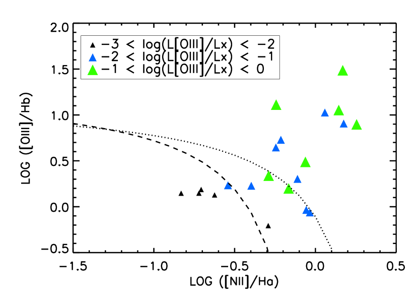
Figure 7.— A BPT diagram for the non-BLAGNs in our $2-8~{}\rm keV$ sample with $z\leq 0.5$. The symbols grow in size and change in color with increasing $L_{\rm[OIII]}$/$L_{X}$, as indicated in the legend. The dashed curve denotes the Kauffmann et al. (2003) division between AGNs (upper-right) and star forming galaxies (lower-left). The dotted curve denotes the Kewley et al. (2001) division between AGNs and extreme starbursts.

Figure 8.— (a) Histogram of the $\log(L_{\rm[OIII]}/L_{X})$ for the $z\leq 0.5$ sources in our $2-8~{}\rm keV$ sample with reliable H$\alpha$ and H$\beta$ flux measurements (solid line— BLAGNs; dashed line— non-BLAGNs). The arrow marks the mean value of the Heckman et al. (2005) extinction-uncorrected [OIII]-bright optically selected sample of Seyfert 1s. (b) Same as (a) but for $\log(L_{\rm[OIII],\,corr}/L_{X})$. The arrow marks the mean value of the Mulchaey et al. (1994) extinction-corrected optically selected sample of Seyfert 1s.

One possible explanation for the low [OIII] emission in some AGNs is extinction from the host galaxy. Indeed, in Figure 5 we see that one of the five BPT SF-dominated non-BLAGNs (stars) significantly increases its $\log(L_{\rm[OIII]}/L_{X})$ value as a result of the extinction correction. However, the other four retain significantly lower $\log(L_{\rm[OIII]}/L_{X})$ values than the mean for the BPT AGN-dominated non-BLAGNs. We note that all five BPT SF-dominated non-BLAGNs have reliable H$\alpha$ and H$\beta$ flux measurements and therefore unique extinction corrections. The small extinction corrections suggest that host galaxy obscuration is not the dominant reason for the low [OIII] emission in the majority of our BPT SF-dominated non-BLAGNs.

Figure 8 also provides support for the idea that applying extinction corrections does not help in reducing the scatter in the ratio between $L_{\rm[OIII]}$ and $L_{X}$. In this figure we show the distribution of (a) $\log(L_{\rm[OIII]}/L_{X})$ and (b) $\log(L_{\rm[OIII],\,corr}/L_{X})$ for the $z\leq 0.5$ BLAGNs in our $2-8~{}\rm keV$ sample (solid line). We also show the distribution for our $z\leq 0.5$ non-BLAGNs (dashed line). We only include sources with reliable H$\alpha$ and H$\beta$ flux measurements. While the numbers are small, we see that correcting for extinction does not reduce the dispersion.

It is possible that the extinction corrections determined from the Balmer line ratios in Section 3.2 are not totally correct for the [OIII] emission. For example, there may be additional contributions to the Balmer emission lines from star formation further out in the galaxy, so if the dust were not mixed uniformly throughout, the extinction corrections measured from the Balmer line ratios might be less than what they should be for the narrow-line region. However, at least the extinction corrections from the Balmer line ratios give some impression of how extinction might alter things, and we see that it does not solve the problem. Another issue is whether X-ray absorption due to an obscuring torus around the AGN could be affecting the luminosity ratio and whether correcting $L_{X}$ for absorption by the torus would reduce the dispersion.

We address these issues in Figure 9, where we show $\log(L_{\rm[OIII]}/L_{X})$ versus $\log$ $L_{X}$ for the BLAGNs in our $2-8$ keV sample as well as for the BLAGNs in other X-ray selected surveys from the literature. We see that a similar high dispersion is also observed for the BLAGNs, even though X-ray absorption would be small and extinction from the galaxy should not be very severe if the AGN is aligned with the disk of the galaxy.

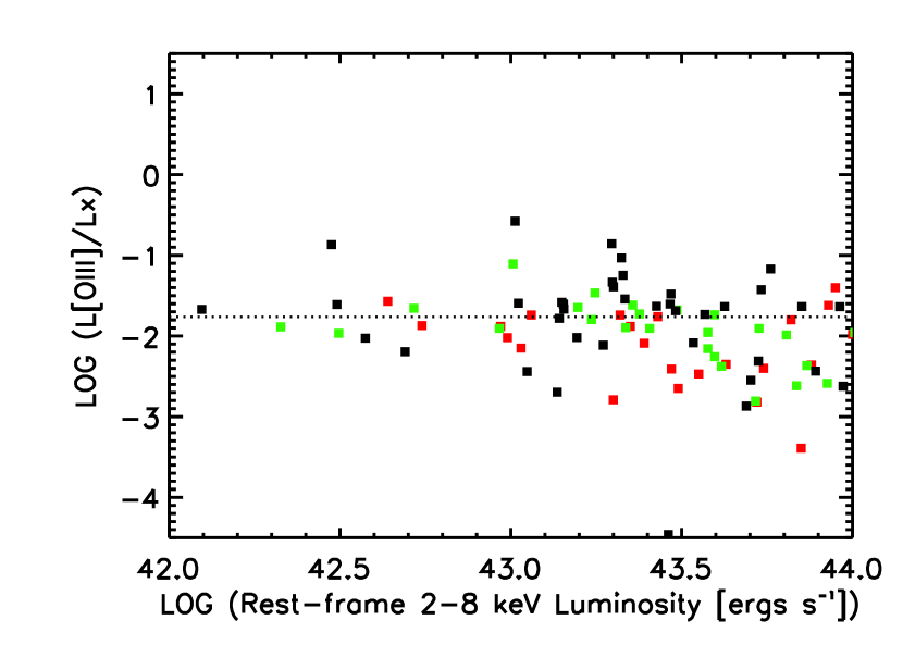
Figure 9.— $\log(L_{\rm[OIII]}/L_{X})$ vs. $\log$ $L_{X}$ for the $L_{X}>10^{42}$ erg s^-1 BLAGNs with $z\leq 0.85$ in our $2-8~{}\rm keV$ sample (black squares). The horizontal dotted line denotes the mean $\langle$$\log(L_{\rm[OIII]}/L_{X})$$\rangle=-1.76$ for these sources. The $L_{\rm[OIII]}$ values are not extinction-corrected. The green squares show the Heckman et al. (2005) sample of $z<0.2$ Seyfert 1s from the RXTE slew survey (Sazonov & Revnivtsev, 2004). The red squares show the Cocchia et al. (2007) Seyfert 1 sample from the HELLAS2XMM survey.

We conclude that sometimes [OIII] will diagnose the presence of an AGN and sometimes it will not, and extinction is not the primary factor. Furthermore, we find that the dispersion in $L_{\rm[OIII]}/L_{X}$ is larger than the dispersion in $L_{\rm opt}/L_{X}$, which suggests that $L_{\rm[OIII]}$ is particularly problematic. We characterize the optical continuum luminosity, $L_{\rm opt}$, in our sources by their rest-frame $g$-band luminosity, $L_{g}$. We determine $L_{g}$ by transforming the observed $g,r,i,z,J,H,K_{s}$ OPTX photometry (Trouille et al., 2008) into $g$-band flux at $z=0$ using kcorrect v4_1_4 (Blanton & Roweis, 2007). Since the contribution from the emission lines in AGNs is so low compared to the continuum luminosity (see Heckman et al. 2004 in which $\langle L_{\rm opt}/L_{\rm[OIII]}\rangle\sim 320$ for SDSS type 1 AGNs), $L_{g}$ provides a reasonable proxy for the optical continuum luminosity in these sources. We find a mean $\log(L_{\rm opt}/L_{X})$ for our BLAGNs of 0.94, with a dispersion of 0.36. This is smaller than the dispersion in $\log(L_{\rm[OIII]}/L_{X})$ ($\sigma=0.5$ for our BLAGNs, see Table 1).

Instead we suggest that there is substantial complexity in the structure of the narrow-line region, which causes many ionizing photons from the AGN not to be absorbed. This complexity could include a low covering fraction of material, the configuration of the HII regions, the presence of density-bounded HII regions, and wind venting. Hence, $L_{\rm[OIII]}/L_{X}$ would be low, and one would perceive the source as a star former rather than as an AGN.

Several groups have compared the hard X-ray and [OIII] luminosity functions (LFs) for AGNs in the local universe (e.g., Heckman et al., 2005; Georgantopoulos & Akylas, 2010) to try to determine which selection of AGN is most efficient. As we have shown, the large dispersion in $L_{\rm[OIII]}/L_{X}$ means that this transformation cannot be done to better than a factor of $\sim 3$ (one sigma) for an individual object. However, even though we cannot be confident about the tranformation, it is still interesting to explore whether the two LFs have, on average, the same shape.

In Figure 10(a) we show the SDSS [OIII] LF for $z<0.15$ Seyfert 2s (Hao et al., 2005, black curve) and $z<0.3$ type 2 quasars (Reyes et al., 2008, blue curve). Following Reyes et al. (2008), we shift the Hao et al. (2005) luminosities by 0.14 dex to account for the difference between the spectrophotometric calibration scales. Reyes et al. (2008) stress that their type 2 quasar LF is a lower limit due to their selection criteria, the details of the spectroscopic target selection, and other factors. On this we show the Sazonov & Revnivtsev (2004) $3-20~{}\rm keV$ LF based on their fit to the local RXTE sample (green curve). We also show the $z=0.1$ (red solid curve; this is the volume-weighted redshift that corresponds to the redshift range of the SDSS Seyfert 2s) and $z=0.2$ (red dashed curve; this is the volume-weighted redshift that corresponds to the redshift range of the SDSS type 2 quasars) extrapolations of the Yencho et al. (2009) best fit to their distant Chandra plus local SWIFT BAT $2-8$ keV sample over the redshift interval $0<z<1.2$ for an independent luminosity and density evolution (ILDE) model. We have transformed the X-ray LFs to the [OIII] LFs using $\langle$$\log(L_{\rm[OIII]}/L_{X})$$\rangle=-1.06$ (from the $z\leq 0.5$ BPT AGN-dominated non-BLAGNs). The gray shading shows the $3~{}\sigma$ uncertainties on the transformation. Since neither Hao et al. (2005) nor Reyes et al. (2008) apply a reddening correction to their [OIII] luminosities, we use our extinction-uncorrected transformation.

The bottom panel shows the transformed Yencho et al. (2009) LFs divided by the SDSS LFs. For $L_{\rm[OIII]}<10^{42}$ erg s^-1, we divide the Yencho et al. (2009) $z=0.1$ LF by the Hao et al. (2005) $z<0.15$ LF. For $L_{\rm[OIII]}\geq 10^{42}$ erg s^-1, we divide the Yencho et al. (2009) $z=0.2$ LF by the Reyes et al. (2008) $z<0.3$ LF.

In Figures 10(b) and (c) we instead did the transformations using $\langle$$\log(L_{\rm[OIII]}/L_{X})$$\rangle=-1.46$ (from the $z\leq 0.5$ non-BLAGNs, excluding the upper limit values for the absorbers) and $\langle$$\log(L_{\rm[OIII]}/L_{X})$$\rangle=-1.85$ (from the $z\leq 0.5$ BLAGNs).

Despite the fact that there are strong selection effects in both the [OIII] and hard X-ray LFs (particularly in the way the [OIII] LFs were constructed, since they contain only Seyfert 2s, and due to the X-ray selection missing heavily X-ray absorbed, Compton-thick sources), we see reasonable agreement. Thus, unlike Heckman et al. (2005), we do not see any evidence for a substantial increase in the [OIII] LF relative to the X-ray LF (see also Georgantopoulos & Akylas, 2010).

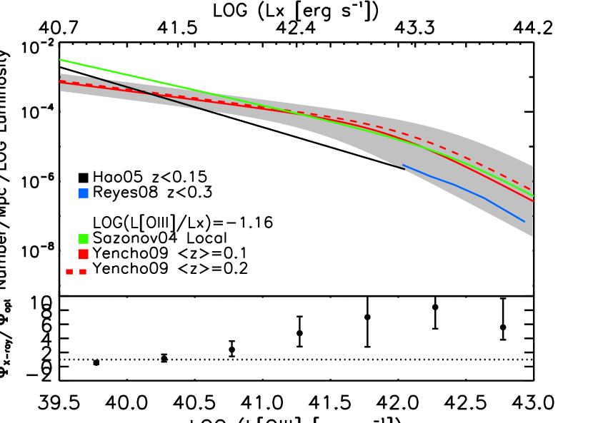
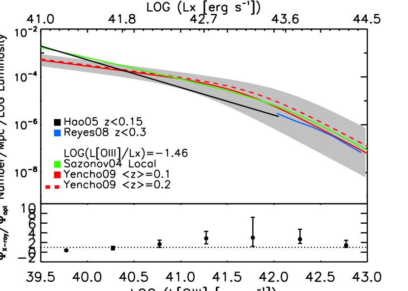
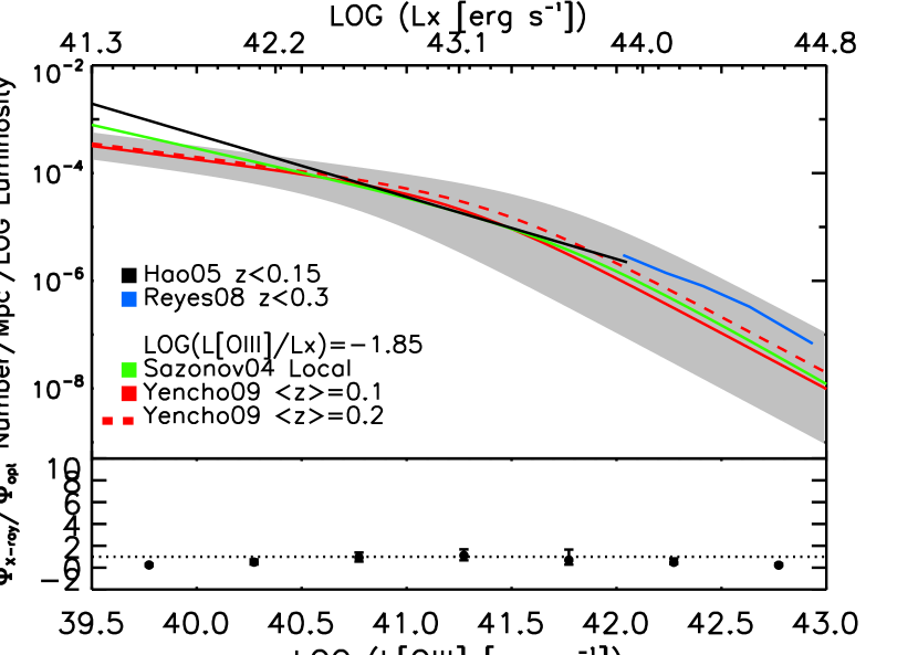
Figure 10.— (a) Comparison of the X-ray and [OIII] LFs (black curve—Hao et al. (2005) [OIII] LF derived from the $z<0.15$ SDSS Seyfert 2s; blue curve—Reyes et al. (2008) [OIII] LF derived from the $z<0.3$ SDSS type 2 quasars; green curve—Sazonov & Revnivtsev (2004) $3-20~{}\rm keV$ local RXTE LF; red curve—Yencho et al. (2009) $z=0.1$ extrapolation to their ILDE model best fit to the $0<z<1.2$ rest-frame $2-8~{}\rm keV$ distant+local LF; red dashed curve—same as the red curve but for a $z=0.2$ extrapolation). We aligned the X-ray LFs to the [OIII] LFs using the BPT AGN-dominated non-BLAGNs $\langle$$\log(L_{\rm[OIII]}/L_{X})$$\rangle=-1.06$. The gray shading shows the $3~{}\sigma$ uncertainties for the transformed Yencho et al. (2009) $z=0.1$ LF. Bottom panel shows the transformed Yencho et al. (2009) X-ray LFs divided by the SDSS LFs. (b) Same as (a) but using the $z\leq 0.5$ non-BLAGNs $\langle$$\log(L_{\rm[OIII]}/L_{X})$$\rangle=-1.46$, which excludes the upper limit values for the absorbers. (c) Same as (a) but using the $z\leq 0.5$ BLAGNs $\langle$$\log(L_{\rm[OIII]}/L_{X})$$\rangle=-1.85$.

7. Summary

We have used our highly optically spectroscopically complete OPTX sample of $2-8$ keV X-ray selected AGNs to see how well an empirical optical emission-line diagnostic diagram does in classifying the X-ray sources as AGNs. We find that roughly 20% of the X-ray AGNs that can be put on these diagrams are not classified as AGNs by the optical diagnostic diagram, if we use the Kauffmann et al. (2003) empirical division between AGN and star formers. If instead we use the Kewley et al. (2001) theoretical division, over half of our X-ray AGNs are not classified as AGNs. We show that both the BLAGNs and the non-BLAGNs in the OPTX sample exhibit a large (two orders in magnitude) dispersion in the ratio of the [OIII] to hard X-ray luminosities, even after the application of reddening corrections to the [OIII] luminosities. This confirms previous results from the literature. The large observed spread in the luminosity ratio leads us to postulate that the X-ray AGNs that are misidentified by the optical diagnostic diagram as star formers have low [OIII] luminosities due to the complexity of the structure of the narrow-line region. If this is indeed the case, then many of the ionizing photons from the AGN are not absorbed, and the [OIII] luminosity can only be used to predict the X-ray luminosity to within a factor of $\sim 3$ (one sigma). While Meléndez et al. (2008), Rigby et al. (2009), and Diamond-Stanic et al. (2009) advocate [OIV] 26 $\mu$m as a more reliable indicator of ionizing flux, it should be similarly affected by the complexity of the structure of the narrow-line region.

References

- Akylas et al. (2006) Akylas, A., Georgantopoulos, I., Georgakakis, A., Kitsionas, S., & Hatziminaoglou, E. 2006, A&A, 459, 693
- Alonso-Herrero et al. (1997) Alonso-Herrero, A., Ward, M. J., & Kotilainen, J. K. 1997, MNRAS, 288, 977
- Antonucci (1993) Antonucci, R. 1993, ARA&A, 31, 473
- Baldwin et al. (1981) Baldwin, J. A., Phillips, M. M., & Terlevich, R. 1981, PASP, 93, 5 (BPT)
- Barger et al. (2002) Barger, A. J., Cowie, L. L., Brandt, W. N., Capak, P., Garmire, G. P., Hornschemeier, A. E., Steffen, A. T., & Wehner, E. H. 2002, AJ, 124, 1839
- Barger et al. (2005) Barger, A. J., Cowie, L. L., Mushotzky, R. F., Yang, Y., Wang, W.-H., Steffen, A. T., & Capak, P. 2005, AJ, 129, 578
- Bassani et al. (1999) Bassani, L., Dadina, M., Maiolino, R., Salvati, M., Risaliti, G., della Ceca, R., Matt, G., & Zamorani, G. 1999, ApJS, 121, 473
- Beckmann et al. (2006) Beckmann, V., Soldi, S., Shrader, C. R., Gehrels, N., & Produit, N. 2006, ApJ, 652, 126
- Blanton & Roweis (2007) Blanton, M. R. & Roweis, S. 2007, AJ, 133, 734
- Bongiorno et al. (2010) Bongiorno, A., Mignoli, M., Zamorani, G., Lamareille, F., Lanzuisi, G., Miyaji, T., Bolzonella, M., Carollo, C. M., Contini, T., Kneib, J. P., Le Fèvre, O., Lilly, S. J., Mainieri, V., Renzini, A., Scodeggio, M., Bardelli, S., Brusa, M., Caputi, K., Civano, F., Coppa, G., Cucciati, O., de La Torre, S., de Ravel, L., Franzetti, P., Garilli, B., Halliday, C., Hasinger, G., Koekemoer, A. M., Iovino, A., Kampczyk, P., Knobel, C., Kovač, K., Le Borgne, J., Le Brun, V., Maier, C., Merloni, A., Nair, P., Pello, R., Peng, Y., Perez Montero, E., Ricciardelli, E., Salvato, M., Silverman, J., Tanaka, M., Tasca, L., Tresse, L., Vergani, D., Zucca, E., Abbas, U., Bottini, D., Cappi, A., Cassata, P., Cimatti, A., Guzzo, L., Leauthaud, A., Maccagni, D., Marinoni, C., McCracken, H. J., Memeo, P., Meneux, B., Oesch, P., Porciani, C., Pozzetti, L., & Scaramella, R. 2010, A&A, 510, A56
- Bruzual & Charlot (2003) Bruzual, G. & Charlot, S. 2003, MNRAS, 344, 1000
- Cocchia et al. (2007) Cocchia, F., Fiore, F., Vignali, C., Mignoli, M., Brusa, M., Comastri, A., Feruglio, C., Baldi, A., Carangelo, N., Ciliegi, P., D’Elia, V., La Franca, F., Maiolino, R., Matt, G., Molendi, S., Perola, G. C., & Puccetti, S. 2007, A&A, 466, 31
- Comastri (2004) Comastri, A. 2004, in Astrophysics and Space Science Library, Vol. 308, Supermassive Black Holes in the Distant Universe, ed. A. J. Barger, 245
- Cowie & Barger (2008) Cowie, L. L. & Barger, A. J. 2008, ApJ, 686, 72
- Dahari & De Robertis (1988) Dahari, O. & De Robertis, M. M. 1988, ApJS, 67, 249
- Diamond-Stanic et al. (2009) Diamond-Stanic, A. M., Rieke, G. H., & Rigby, J. R. 2009, ApJ, 698, 623
- Faber et al. (2003) Faber, S. M., Phillips, A. C., Kibrick, R. I., Alcott, B., Allen, S. L., Burrous, J., Cantrall, T., Clarke, D., Coil, A. L., Cowley, D. J., Davis, M., Deich, W. T. S., Dietsch, K., Gilmore, D. K., Harper, C. A., Hilyard, D. F., Lewis, J. P., McVeigh, M., Newman, J., Osborne, J., Schiavon, R., Stover, R. J., Tucker, D., Wallace, V., Wei, M., Wirth, G., & Wright, C. A. 2003, Proc. SPIE, 4841, 1657
- Ferland & Netzer (1983) Ferland, G. J. & Netzer, H. 1983, ApJ, 264, 105
- Ferland & Osterbrock (1986) Ferland, G. J. & Osterbrock, D. E. 1986, ApJ, 300, 658
- Ferruit et al. (1999) Ferruit, P., Wilson, A. S., Whittle, M., Simpson, C., Mulchaey, J. S., & Ferland, G. J. 1999, ApJ, 523, 147
- Georgantopoulos & Akylas (2010) Georgantopoulos, I. & Akylas, A. 2010, A&A, 509, A26
- Guainazzi et al. (2005) Guainazzi, M., Matt, G., & Perola, G. C. 2005, A&A, 444, 119
- Hao et al. (2005) Hao, L., Strauss, M. A., Fan, X., Tremonti, C. A., Schlegel, D. J., Heckman, T. M., Kauffmann, G., Blanton, M. R., Gunn, J. E., Hall, P. B., Ivezić, Ž., Knapp, G. R., Krolik, J. H., Lupton, R. H., Richards, G. T., Schneider, D. P., Strateva, I. V., Zakamska, N. L., Brinkmann, J., & Szokoly, G. P. 2005, AJ, 129, 1795
- Hasinger (2008) Hasinger, G. 2008, A&A, 490, 905
- Heckman et al. (2004) Heckman, T. M., Kauffmann, G., Brinchmann, J., Charlot, S., Tremonti, C., & White, S. D. M. 2004, ApJ, 613, 109
- Heckman et al. (2005) Heckman, T. M., Ptak, A., Hornschemeier, A., & Kauffmann, G. 2005, ApJ, 634, 161
- Kakazu et al. (2007) Kakazu, Y., Cowie, L. L., & Hu, E. M. 2007, ApJ, 668, 853
- Kauffmann et al. (2003) Kauffmann, G., Heckman, T. M., Tremonti, C., Brinchmann, J., Charlot, S., White, S. D. M., Ridgway, S. E., Brinkmann, J., Fukugita, M., Hall, P. B., Ivezić, Ž., Richards, G. T., & Schneider, D. P. 2003, MNRAS, 346, 1055
- Kewley et al. (2001) Kewley, L. J., Dopita, M. A., Sutherland, R. S., Heisler, C. A., & Trevena, J. 2001, ApJ, 556, 121
- Kewley et al. (2006) Kewley, L. J., Groves, B., Kauffmann, G., & Heckman, T. 2006, MNRAS, 372, 961
- La Franca et al. (2005) La Franca, F., Fiore, F., Comastri, A., Perola, G. C., Sacchi, N., Brusa, M., Cocchia, F., Feruglio, C., Matt, G., Vignali, C., Carangelo, N., Ciliegi, P., Lamastra, A., Maiolino, R., Mignoli, M., Molendi, S., & Puccetti, S. 2005, ApJ, 635, 864
- La Massa et al. (2009) La Massa, S. M., Heckman, T. M., Ptak, A., Hornschemeier, A., Martins, L., Sonnentrucker, P., & Tremonti, C. 2009, ApJ, 705, 568
- Laurent-Muehleisen et al. (1998) Laurent-Muehleisen, S. A., Kollgaard, R. I., Ciardullo, R., Feigelson, E. D., Brinkmann, W., & Siebert, J. 1998, ApJS, 118, 127
- Lawrence & Elvis (1982) Lawrence, A. & Elvis, M. 1982, ApJ, 256, 410
- Magnelli et al. (2009) Magnelli, B., Elbaz, D., Chary, R. R., Dickinson, M., Le Borgne, D., Frayer, D. T., & Willmer, C. N. A. 2009, A&A, 496, 57
- Meléndez et al. (2008) Meléndez, M., Kraemer, S. B., Armentrout, B. K., Deo, R. P., Crenshaw, D. M., Schmitt, H. R., Mushotzky, R. F., Tueller, J., Markwardt, C. B., & Winter, L. 2008, ApJ, 682, 94
- Moran et al. (1999) Moran, E. C., Lehnert, M. D., & Helfand, D. J. 1999, ApJ, 526, 649
- Mulchaey et al. (1994) Mulchaey, J. S., Koratkar, A., Ward, M. J., Wilson, A. S., Whittle, M., Antonucci, R. R. J., Kinney, A. L., & Hurt, T. 1994, ApJ, 436, 586
- Netzer et al. (2006) Netzer, H., Mainieri, V., Rosati, P., & Trakhtenbrot, B. 2006, A&A, 453, 525
- Osterbrock & Martel (1993) Osterbrock, D. E. & Martel, A. 1993, ApJ, 414, 552
- Osterbrock & Pogge (1985) Osterbrock, D. E. & Pogge, R. W. 1985, ApJ, 297, 166
- Ptak et al. (2006) Ptak, A., Zakamska, N. L., Strauss, M. A., Krolik, J. H., Heckman, T. M., Schneider, D. P., & Brinkmann, J. 2006, ApJ, 637, 147
- Ranalli et al. (2003) Ranalli, P., Comastri, A., & Setti, G. 2003, A&A, 399, 39
- Reyes et al. (2008) Reyes, R., Zakamska, N. L., Strauss, M. A., Green, J., Krolik, J. H., Shen, Y., Richards, G. T., Anderson, S. F., & Schneider, D. P. 2008, AJ, 136, 2373
- Rigby et al. (2009) Rigby, J. R., Diamond-Stanic, A. M., & Aniano, G. 2009, ApJ, 700, 1878
- Sazonov et al. (2007) Sazonov, S., Revnivtsev, M., Krivonos, R., Churazov, E., & Sunyaev, R. 2007, A&A, 462, 57
- Sazonov & Revnivtsev (2004) Sazonov, S. Y. & Revnivtsev, M. G. 2004, A&A, 423, 469
- Silverman et al. (2008) Silverman, J. D., Green, P. J., Barkhouse, W. A., Kim, D.-W., Kim, M., Wilkes, B. J., Cameron, R. A., Hasinger, G., Jannuzi, B. T., Smith, M. G., Smith, P. S., & Tananbaum, H. 2008, ApJ, 679, 118
- Simpson (2005) Simpson, C. 2005, MNRAS, 360, 565
- Stasińska et al. (2006) Stasińska, G., Cid Fernandes, R., Mateus, A., Sodré, L., & Asari, N. V. 2006, MNRAS, 371, 972
- Steffen et al. (2003) Steffen, A. T., Barger, A. J., Cowie, L. L., Mushotzky, R. F., & Yang, Y. 2003, ApJ, 596, L23
- Szokoly et al. (2004) Szokoly, G. P., Bergeron, J., Hasinger, G., Lehmann, I., Kewley, L., Mainieri, V., Nonino, M., Rosati, P., Giacconi, R., Gilli, R., Gilmozzi, R., Norman, C., Romaniello, M., Schreier, E., Tozzi, P., Wang, J. X., Zheng, W., & Zirm, A. 2004, ApJS, 155, 271
- Tremonti et al. (2004) Tremonti, C. A., Heckman, T. M., Kauffmann, G., Brinchmann, J., Charlot, S., White, S. D. M., Seibert, M., Peng, E. W., Schlegel, D. J., Uomoto, A., Fukugita, M., & Brinkmann, J. 2004, ApJ, 613, 898
- Trouille et al. (2008) Trouille, L., Barger, A. J., Cowie, L. L., Yang, Y., & Mushotzky, R. F. 2008, ApJS, 179, 1
- Trouille et al. (2009) —. 2009, ApJ, 703, 2160
- Ueda et al. (2003) Ueda, Y., Akiyama, M., Ohta, K., & Miyaji, T. 2003, ApJ, 598, 886
- Veilleux & Osterbrock (1987) Veilleux, S. & Osterbrock, D. E. 1987, ApJS, 63, 295
- Weedman (1977) Weedman, D. W. 1977, ARA&A, 15, 69
- Weedman (1978) —. 1978, MNRAS, 184, 11P
- Winter et al. (2009) Winter, L. M., Mushotzky, R. F., Reynolds, C. S., & Tueller, J. 2009, ApJ, 690, 1322
- Yencho et al. (2009) Yencho, B., Barger, A. J., Trouille, L., & Winter, L. M. 2009, ApJ, 698, 380
- Zakamska et al. (2003) Zakamska, N. L., Strauss, M. A., Krolik, J. H., Collinge, M. J., Hall, P. B., Hao, L., Heckman, T. M., Ivezić, Ž., Richards, G. T., Schlegel, D. J., Schneider, D. P., Strateva, I., Vanden Berk, D. E., Anderson, S. F., & Brinkmann, J. 2003, AJ, 126, 2125
- Zezas et al. (1998) Zezas, A. L., Georgantopoulos, I., & Ward, M. J. 1998, MNRAS, 301, 915