Role of the mean curvature in the geometry of magnetic confinement configurations

Abstract

Examples are presented of how the geometric notion of the mean curvature is used for general magnetic field configurations and magnetic surfaces. It is shown that the mean magnetic curvature is related to the variation of the absolute value of the magnetic field along its lines. Magnetic surfaces of constant mean curvature are optimum for plasma confinement in multimirror open confinement systems and rippled tori.

Introduction

The mean curvature is one of the basic notions in the geometry of surfaces and vector fields [1, 2], while the geometry of magnetic fields, as applied to the problems of fusion plasma confinement, does not in fact invoke this notion (as is confirmed in [3]). The object of the present methodological note is to bridge this gap. We begin by giving the definitions and main results on the differential geometry of surfaces in three-dimensional Euclidean space and of vector fields and then present various applications of the notion of mean curvature in magnetic confinement systems.

1 Mean curvature of surfaces and vector fields

The mean curvature of a surface, $H_{S}$, is a local quantity defined by the formula

$$H_{S}=-\frac{1}{2}(k_{\mathrm{min}}+k_{\mathrm{max}}),$$

where $k_{\mathrm{min}}$ and $k_{\mathrm{max}}$ are the minimum and maximum curvatures of the lines of intersection of the surface with mutually perpendicular planes passing through the normal to the surface at its given point. For ${\bf{e}}\cdot(\nabla\times{\bf{e}})=0$, draw a family of surface orthogonal to a unit vector field ${\bf{e}}$ (such that $|{\bf{e}}|=1$). The mean curvature of these surfaces is called the mean curvature of the vector field ${\bf{e}}$. In the general case ${\bf{e}}\cdot(\nabla\times{\bf{e}})\neq 0$ and the mean curvature $H$ of a vector field ${\bf{e}}$ is defined by the formula [2]

$$H=-\frac{1}{2}\nabla\cdot{\bf{e}}.$$

For a unit vector ${\bf{e}}={\bf{n}}$ along the normal ${\bf{n}}$ to a surface, the general definition of the curvature $H$ coincides with that of $H_{S}$ (see the definition (1)). The surface of zero mean curvature, $H_{S}=0$, is called a minimal surface. Examples of minimal surfaces are given by surfaces of minimum area $S$ with a fixed boundary (soap films). Closed minimal surfaces do not exist. Among surfaces of constant mean curvature $H_{S}=\mathrm{const}$ are soap films between media at different pressures $p$, in which case the mean curvature is just the pressure difference. Another example of the surfaces of constant mean curvature $H_{S}=\mathrm{const}$ are those among the surfaces bounding regions of given volume $V$ that have a minimum area $S$. Such surfaces are called isoperimetric profiles and are perfect spheres of constant curvature. The Aleksandrov theorem [4] states that such spheres are the only embedded (or nested, i.e. non-self-intersecting) closed surfaces of constant mean curvature. A consequence of the theorem is, in particular, that embedded (nested) tori of constant mean curvature do not exist.

The statement of this general theorem can be simply verified for surfaces of revolution. Assuming that the axis of revolution is the $Z$ axis of a cylindrical coordinate system, we specify the shape of a surface of revolution by the equation $\Phi=z-z(r)$. Substituting the normal to this surface, ${\bf{n}}=\nabla\Phi/|\nabla\Phi|$, into (2), we obtain the equation

$$2H_{S}=\frac{1}{r}\frac{d}{dr}\left(\frac{rz^{\prime}}{\sqrt{1+z^{\prime 2}}}\right),$$

where the prime denotes the derivative with respect to the radius $r$. For a constant mean curvature, Eq. (3) is integrable:

$$H_{S}r^{2}+C=\frac{rz^{\prime}}{\sqrt{1+z^{\prime 2}}},$$

where $C$ is a constant of integration. Equations (3) and (4) imply that a closed plane curve having two or more points where $z^{\prime}=0$ at $r>0$ does not exist. Consequently, a torus of constant mean curvature is impossible. Unfortunately, in considering an axisymmetric example in [5], sad mistakes were made that led to an erroneous conclusion about the existence a torus of constant mean curvature.

Equation (4) shows that there may be two points where $z^{\prime}=\infty$ at $r>0$. The generating contours of these surfaces of revolution are described by a focus of a hyperbola or an ellipse (see Fig. 1) rolled along the straight axis of revolution [6].

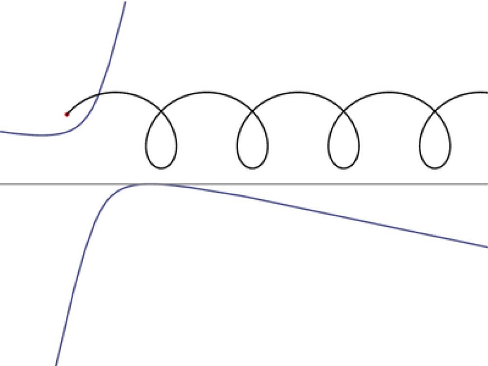
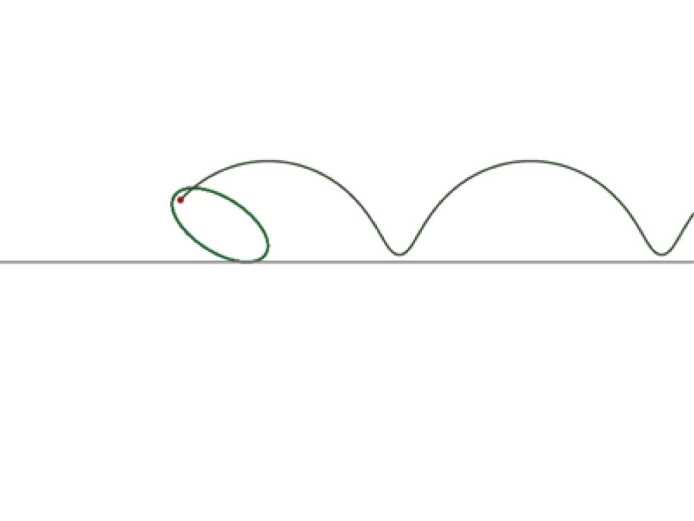
Figure 1: Rolling of hyperbola and ellipse.

A cylinder is a limiting case of rolling of a circle. This demonstrates the existence of surfaces with $H_{S}=\mathrm{const}$ that are periodic along the axis of revolution (see Fig. 2).

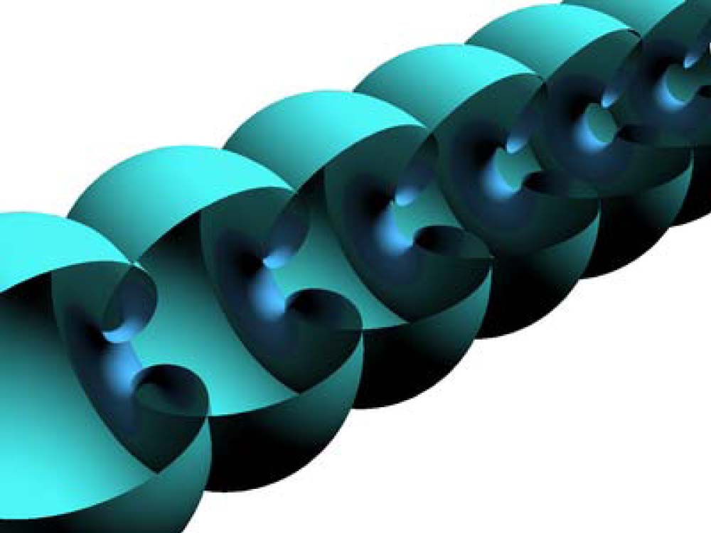
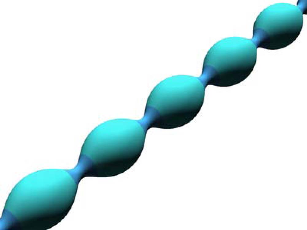
Figure 2: Nodoid and unduloid.

In the theory of surfaces, the Willmore functional determined by an integral of the square of the mean curvature over a surface plays an important role. For closed surfaces, this functional is conformally invariant: in a conformal mapping of a three-dimensional space onto itself, the values of the Willmore functional on a surface and on its transform coincide [7]. This functional not only plays a key role in the Weierstrass representation of surfaces [7] but has recently come into use in biophysics and colloidal chemistry—disciplines in which it is known as the Helfrich functional [8]. The critical points of the Helfrich functional generate Willmore surfaces [7]. In contrast to minimal surfaces, there are many examples of closed Willmore surfaces, including embedded (non-self-intersecting) ones. Among them are, e.g., all spheres of constant curvature and also a Clifford torus — a surface of revolution generated by revolving such circle about its axis that the ratio of the distance $R$ between the center of the circle and the axis of revolution to the circle radius $r$ is $\sqrt{2}$.

2 Mean curvature of a magnetic field

According to (2), a magnetic field ${\bf B}=B\cdot{\bf{b}}$, where $|{\bf{b}}|=1$ and $B=|{\bf B}|$ is the absolute value of fiel, can be characterized by the mean curvature

$$H_{b}={\bf{b}}\cdot\nabla\log\sqrt{B}.$$

The variation of the absolute value of the magnetic field along its lines is an important parameter of plasma magnetic confinement systems and is often used in the geometry of magnetic fields [3, 9]. For a vacuum magnetic field ${\bf B}=-\nabla\varphi$, where $\varphi$ is the scalar magnetic potential, the mean curvature $H_{b}$ coincides with that of an equipotential surface $\varphi=\mathrm{const}$ for which the vector ${\bf{b}}$ is a unit normal vector. Note that, by (2), the expression (5) for the mean curvature is also valid for $\nabla\times{\bf B}\neq 0$.

At the extreme points of the absolute value of the magnetic field along its lines, we have $H_{b}=0$. In the so-called isodynamic toroidal configurations revealed by D. Palumbo [10], the absolute value of the magnetic field is constant on the nested magnetic surfaces, $B=\mathrm{const}$, so the mean curvature is zero: $H_{b}=0$, over the entire confinement region. Such isodynamic toroidal configurations are possible only in the presence of the discharge current [11]. Without the discharge current, i.e., in vacuum, the equipotential surfaces in an isodynamic configuration should be minimal, which is impossible, however, in view of the results obtained by Palumbo [11].

The magnetic fields that form a family of nested magnetic surfaces, ${\bf B}\cdot{\bf{n}}=0$, in a finite spatial region play a governing role in plasma confinement. Magnetic configurations for plasma confinement can be divided into open configurations with rippled cylindrical nested magnetic surfaces and closed configurations with nested toroidal magnetic surfaces of complicated shape. The solenoidal nature of the magnetic field implies that the toroidal magnetic flux $\Phi$ within a magnetic surface is conserved. This is why the most general equation for a family of nested magnetic surfaces is formulated in terms of the toroidal magnetic flux: $\Phi(x,y,z)=\mathrm{const}$. The function $\Phi$ is a single-valued solution, if there is any, to the equation ${\bf B}\cdot\nabla\Phi=0$ with a known magnetic field having a nonzero rotational transform. Hence, at each point of the plasma confinement region, the vector field of unit vectors normal to the magnetic surfaces, ${\bf{n}}=\nabla\Phi/|\nabla\Phi|$ such that ${\bf{n}}\cdot(\nabla\times{\bf{n}})=0$, is usually defined. By substituting the vector ${\bf{n}}$ into (2), it is possible to determine the mean curvature $H_{S}$ of the magnetic surfaces—a quantity that plays an important role in the theory of plasma confinement systems.

For completeness sake, we supplement the vectors ${\bf{b}}$ and ${\bf{n}}$, which have been introduced above, with the binormal vector ${\bf{t}}={\bf{b}}\times{\bf{n}}$ up to an orthonormalized magnetic basis. The vector ${\bf{t}}$ is directed along the vector ${\bf B}\times\nabla\Phi$, which is orthogonal to ${\bf B}$. In an equilibrium state in which the plasma currents ${\bf{j}}$ flow along the magnetic surfaces ${\bf{j}}\cdot\nabla\Phi=0$ the vector ${\bf B}\times\nabla\Phi$ is solenoidal and its lines lie on the magnetic surfaces [9]. Applying (2) to ${\bf{t}}$ defines the mean curvature of the additional field:

$$H_{t}={\bf{t}}\cdot\nabla\log\sqrt{B|\nabla\Phi|}.$$

This curvature is related to such familiar parameter as the geodesic curvature of the magnetic field lines [9].

2.1 Magnetic surfaces with $H=\mathrm{const}$

The energy and particle confinement in magnetic systems is commonly characterized by integral confinement times. For definiteness, let us consider the particle confinement time $\tau_{N}$. This time is calculated from the formula $\tau_{N}=N/I$, where $N$ is the total number of particles in the system after the injection of the particle current $I$. In turn, the total number of particles is $N=nV$, where $n$ is the mean particle density in the system and $V$ is its volume. Since, in a steady state, the injection current is equal to the loss current, we have $I=nvS$, where $v$ is the mean velocity with which the particles escape from the system through a boundary region of area $S$. As a result, the particle confinement time is given by the formula $\tau_{N}=V/vS$. The better the confinement, the longer this time. Under the assumption that $v$ is constant, we arrive at the conclusion that the boundary surfaces of constant mean curvature are optimum for plasma confinement.

As shown in Section 1, there exist periodic axisymmetric unduloid surfaces with $H_{S}=\mathrm{const}$ (see Fig. 2) that can be used to optimize plasma confinement in ambipolar open magnetic systems [9]. The central solenoid of such configurations with a straight magnetic axis is characterized by the length $L$ and on-axis mirror ratio $P=B_{\mathrm{max}}/B_{\mathrm{min}}$, or the ratio of the maximum and minimum radii $r_{\mathrm{max}}/r_{\mathrm{min}}=\sqrt{P}$. The values of $L$ and $P$ determine the parameters of an ellipse that generates an optimum unduloid for a given geometry of the magnetic configuration.

In Section 1, it was pointed out that tori with $H_{S}=\mathrm{const}$ do not exist. It is, however, for an ambipolar open magnetic confinement system that we consider asymptotic surfaces of constant mean curvature. Figure 3 shows a way how to close open systems by means of the magnetic surface of a Kadomtsev rippled confinement system [12].

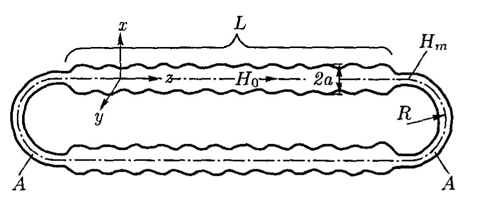
Figure 3: The Kadomtsev confinement system.

Let us modify the Kadomtsev system as follows. On two long straight portions, it is possible to use unduloids with a relatively weak mean magnetic field, and curvilinear elements can be half-tori with a magnetic field strong enough for the radius of the tori to be small. The system can also be arranged to have a square shape: four straight portions with unduloids are closed by curvilinear elements in the form of quarter-tori. This method of modifying the Kadomtsev system can be repeated over and over again. The main idea is that, for a sufficiently large ratio $L/L_{c}$, where $L_{c}$ is the length of the curvilinear elements, and a sufficiently large mirror ratio $P=B_{c}/B$, where $B_{c}$ is the magnetic field in a curvilinear element, the ratio $V/S$ is asymptotically determined only by the straight portions of the system.

2.2 Calculation of the shape of the magnetic Surfaces

The main plasma confinement problem is to calculate a distortion of the shape of the magnetic surfaces that are in equilibrium with a plasma of isotropic pressure, $p=p(\Phi)$. The pressure is assumed to be constant on the magnetic surfaces because it is equalized by a mechanism associated with the fast motion of charged plasma particles along magnetic field lines with irrational rotational transforms. An increase in pressure distorts the magnetic surfaces and, as a rule, destroys their nested structure, thereby deteriorating the plasma confinement radically. This is why solving such problems is aimed at determining the maximum volume-averaged value of the parameter $\beta_{\mathrm{eq}}\sim\left\langle\frac{p}{B^{2}}\right\rangle$ that is consistent with equilibrium. This maximum beta value, and consequently, the plasma confinement efficiency, is very sensitive to the geometric shape of the magnetic surfaces. To be specific, we can mention innovative stellarators with a complicated three-dimensional geometry of helical tori—devices in which the maximum $\beta_{\mathrm{eq}}$ values are more than an order of magnitude higher than those in tokamaks (see [9] for comparison). That is why it is important to search for special geometries of magnetic confinement systems. In this way, it may be very helpful to use Eq. (2) written for the normal to a magnetic surface in the form of an elliptic equation for determining $\Phi(x,y,z)$ at given $|\nabla\Phi|$ and $H_{S}$:

$$\nabla\cdot\left(\frac{\nabla\Phi}{|\nabla\Phi|}\right)=-2H_{S}.$$

Let us introduce the function $\delta=\Phi/|\nabla\Phi|$ which is in fact the distance between neighboring magnetic surfaces. The function $\delta$ so introduced is required to calculate the magnetic field ${\bf B}$ on a given magnetic surface [13]. Instead of $\delta$, it is possible to use the absolute value of the magnetic field $B$ [14]. This is why the choice of the function $|\nabla\Phi|$ is largely determined by how the absolute value of the magnetic field varies along its lines. Moreover, the pseudosymmetry condition, which is now widely used to synthesize innovative stellarators, is also constructed based on the geometry of isomagnetic surfaces (i.e., the surfaces of constant magnetic field strength $B$) [9].

The function $H_{S}$ determines the geometry of the confinement system. From an expression obtained in [14], specifically,

$$H_{S}=\frac{\kappa_{n}+\hat{\kappa}_{n}}{2},$$

where $\kappa_{n}$ and $\hat{\kappa}_{n}$ are the normal curvatures of the lines of the magnetic field ${\bf B}$ and its complement ${\bf B}\times\nabla\Phi$, it is clear that the pressure $p$ enters Eq. (7) through the mean curvature. In fact, the (equilibrium) force balance equation yields the equalities

$$\kappa_{n}=\frac{1}{B^{2}}{\bf{n}}\cdot\nabla\left(p+\frac{B^{2}}{2}\right)=\frac{|\nabla\Phi|}{B^{2}}\,\frac{dp}{d\Phi}+{\bf{n}}\cdot\nabla\log B.$$

The expression for $\hat{\kappa}_{n}={\bf{n}}\cdot({\bf{t}}\cdot\nabla){\bf{t}}$ takes the simplest form for axisymmetric currentless configurations [15]:

$$\hat{\kappa}_{n}=-\ \cdot\nabla\log\frac{|\nabla\Phi|}{B}=-{\bf{n}}\cdot\nabla\log\frac{|\nabla\Phi|}{B^{2}}-{\bf{n}}\cdot\nabla\log B.$$

Simple manipulations put Eq. (7) into the form

$$\nabla\cdot\frac{\nabla\Phi}{(|\nabla\Phi|^{2}/B^{2})}=-\frac{dp}{d\Phi}.$$

Since, in cylindrical coordinates, we have $|\nabla\Phi|^{2}/B^{2}=r^{2}$ up to constants, we arrive at the Grad–Shafranov equation.

Hence, after some algebraic manipulations, Eq. (7) can be used not only to search for an optimum geometry of the boundary magnetic surface but also to solve equilibrium problems.

2.3 The integral $\oint_{S}H_{S}dS$ on nested magnetic surfaces

Let us consider the radial variation of the integral $\oint_{S}H_{S}dS$. To do this, we use the divergent expression presented in [2] for the Gaussian curvature $K$ of a unit vector field ${\bf{e}}$:

$$K=\frac{1}{2}\nabla\cdot(2H{\bf{e}}+\kappa).$$

where $\kappa=-{\bf{e}}\times(\nabla\times{\bf{e}})$ is the curvature vector of the lines of the vector field ${\bf{e}}$. Setting ${\bf{e}}={\bf{n}}$, where ${\bf{n}}$ is the normal to a family of nested magnetic surfaces $\Phi$, and integrating the curvature from formula (12) over the volume $dV=\frac{dS\,d\Phi}{|\nabla\Phi|}$ between two neighboring magnetic surfaces $\Phi$ and $\Phi+d\Phi$, we obtain the equalities

$$\oint_{V}KdV=d\Phi\oint_{S}\frac{K}{|\nabla\Phi|}dS=d\oint_{S}H_{S}dS.$$

Here, we have used the fact that the magnetic flux between the surfaces is constant, $d\Phi=\mathrm{const}$. The result is

$$\frac{d\oint_{S}H_{S}dS}{d\Phi}=\oint_{S}\frac{K}{|\nabla\Phi|}dS.$$

Since $\oint_{S}KdS=0$ for toroidal surfaces, and since $|\nabla\Phi|\approx\mathrm{const}$, the integral on the right-hand side of formula (14) vanishes.

Conclusions

The mean curvature of the magnetic field vector is related to the variation of the absolute value of the magnetic field along its lines. In the presence of magnetic surfaces and, consequently, of the orthonormalized magnetic basis (${\bf{b}},{\bf{n}},{\bf{t}}$), the mean curvature can be introduced for each basis vector. The mean curvature of the normal vector coincides with that of the magnetic surface. Magnetic surfaces of constant mean curvature, having a minimum surface area at a fixed volume, are optimum for plasma confinement in multimirror open systems and rippled tori with straight portions. By specifying the mean curvature of the magnetic surfaces and the distance to the nearest magnetic surface, it is possible to calculate the shape of the magnetic surfaces. All this goes to show that it may be helpful to use the notion of the mean curvature in the geometry of magnetic fields in plasma magnetic confinement systems.

Acknowledgments. We are grateful to N. Schmitt for permission to borrow Figs. 1 and 2. This work was supported in part by the Russian Foundation for Basic Research, the Federal Special-Purpose Program “Scientific and Pedagogical Personnel of the Innovative Russia for 2009–2012”, Presidium of the Russian Academy of Sciences (under the program ”Fundamental Problems of Nonlinear Dynamics”), and the Council of the Russian Federation Presidential Grants for State Support of Leading Scientific Schools (project no. NSh-65382.2010.2).

References

- [1] Novikov, S.P., and Taimanov, I.A.: Modern Geometrical Structures and Fields, Graduate Studies in Math., V. 71, Amer. Math. Soc., Providence, 2006.
- [2] Aminov, Yu.A.: Geometry of Vector Fields, Nauka, Moscow, 1990 [in Russian].
- [3] Morozov, A.I., and Solov’ev, L.S.: in Reviews of Plasma Physics, Ed. by M. A. Leontovich (Gosatomizdat, Moscow, 1963; Consultants Bureau, New York, 1966), Vol. 2.
- [4] Aleksandrov, A.D.: Vestn. Leningr. Univ. 11, 5 (1956).
- [5] Skovoroda, A.A.: Plasma Phys. Rep. 35, 619 (2009) .
- [6] Kenmotsu, K.: Surfaces with Constant Mean Curvature, Transl. of Mathematical Monographs, V. 221, Amer. Math. Soc., Providence, 2003.
- [7] Taimanov, I.A.: Russian Math. Surveys 61:1, 79 (2006).
- [8] Helfrich, W.: Z. Naturforsch. 23, 693 (1973).
- [9] Skovoroda, A.A.: Magnetic Confinement Systems, Fizmatlit, Moscow, 2009 [in Russian].
- [10] Palumbo, D.: Nuovo Cimento 53, 507 (1968).
- [11] Palumbo, D.: Atti Accad. Sci. Lett. Arti Palermo 4, 475 (1983–1984).
- [12] Kadomtsev, B.B.: Selected Articles, Fizmatlit, Moscow, 2003, Vol. 1, p. 35 [in Russian].
- [13] Boozer, A.: Phys. Plasmas 9, 3762 (2002).
- [14] Skovoroda, A.A.: Plasma Phys. Rep. 32, 977 (2006) .
- [15] Skovoroda, A.A.: Plasma Phys. Rep. 35, 99 (2009) .