Coordinated NIR/mm observations of flare emission from Sagittarius A*

Abstract

Context. We report on a successful, simultaneous observation and modelling of the millimeter (mm) to near-infrared (NIR) flare emission of the Sgr A* counterpart associated with the supermassive (4$\times$10⁶ M_⊙ ) black hole at the Galactic centre (GC). We present a mm/sub-mm light curve of Sgr A* with one of the highest quality continuous time coverages.

Aims. We study and model the physical processes giving rise to the variable emission of Sgr A*.

Methods. Our non-relativistic modelling is based on simultaneous observations carried out in May 2007 and 2008, using the NACO adaptive optics (AO) instrument at the ESO’s VLT and the mm telescope arrays CARMA in California, ATCA in Australia, and the 30 m IRAM telescope in Spain. We emphasize the importance of multi-wavelength simultaneous fitting as a tool for imposing adequate constraints on the flare modelling. We present a new method for obtaining concatenated light curves of the compact mm-source Sgr A* from single dish telescopes and interferometers in the presence of significant flux density contributions from an extended and only partially resolved source.

Results. The observations detect flaring activity in both the mm domain and the NIR. Inspection and modelling of the light curves show that in the case of the flare event on 17 May 2007, the mm emission follows the NIR flare emission with a delay of 1.5$\pm$0.5 hours. On 15 May 2007, the NIR flare emission is also followed by elevated mm-emission. We explain the flare emission delay by an adiabatic expansion of source components. For two other NIR flares, we can only provide an upper limit to any accompanying mm-emission of about 0.2 Jy. The derived physical quantities that describe the flare emission give a source component expansion speed of $v_{\mathrm{exp}}$ $\sim$ 0.005$c$ - 0.017$c$, source sizes of about one Schwarzschild radius, flux densities of a few Janskys, and spectral indices of $\alpha$=0.6 to 1.3. These source components peak in the THz regime.

Conclusions. These parameters suggest that either the adiabatically expanding source components have a bulk motion greater than $v_{\mathrm{exp}}$ or the expanding material contributes to a corona or disk, confined to the immediate surroundings of Sgr A*. Applying the flux density values or limits in the mm- and X-ray domain to the observed flare events constrains the turnover frequency of the synchrotron components that are on average not lower than about 1 THz, such that the optically thick peak flux densities at or below these turnover frequencies do not exceed, on average, about $\sim$1 Jy.

1 Introduction

Sgr A*, the compact non-thermal radio and infrared source at the centre of the Milky Way galaxy ($\sim$8 kpc away) is known to be associated with a supermassive black hole (SMBH) of mass $\sim$4$\times$10⁶ M_⊙ (Eckart & Genzel 1996; Genzel et al. 1997, 2000; Ghez et al. 1998, 2000, 2004b, 2004a, 2005; Eckart et al. 2002; Schödel et al. 2002, 2003; Eisenhauer et al. 2003, 2005; Gillessen et al. 2009; Ghez et al. 2009). The close proximity of Sgr A* makes it ideal for studying the evolution and physics of SMBHs located in the nuclei of galaxies. The SMBH radiates far below its Eddington luminosity at all wavelengths, partly because of its low observed accretion rate. For Sgr A*, we assume that $R_{s}$=2$R_{g}$=2$GM$/$c$²$\sim$9 $\mu$as, $R_{s}$ being one Schwarzschild radius and $R_{g}$ the gravitational radius of the SMBH.
Evidence of flaring activity occurring from a few hours to days has been found from variability studies ranging from the radio to sub-mm wavelengths (Bower et al. 2002; Herrnstein et al. 2004; Zhao et al. 2003, 2004; Mauerhan et al. 2005). There is also evidence that variations in radio/sub-mm emission are linked to NIR/X-ray flares, with the radio/sub-mm flares occurring after a delay of $\sim$100 minutes after the NIR/X-ray flares (Eckart et al. 2008b, 2006a, 2004; Marrone et al. 2008; Yusef-Zadeh et al. 2008).

These flares have been explained with a synchrotron self Compton (SSC) model that involves up-scattered sub-mm photons from a compact (inferred from short flare timescales) source component (e.g., Eckart et al. 2004, Eckart et al. 2006a). The X-ray emission is caused by the inverse Compton scattering of the THz-peaked flare spectrum by relativistic electrons. Both synchrotron and SSC mechanisms contribute to NIR flux density. Adiabatic expansion of the source components then gives rise to flares in the mm/sub-mm regimes (Eckart et al. 2006a; Yusef-Zadeh et al. 2006a, b, 2008; Marrone et al. 2008).

Based on the assigned VLT time, we organized an extensive multi-frequency campaign in May 2007 and May 2008 which included millimeter to NIR observations at single telescopes and interferometers around the world. We present data from observations of Sgr A* using CARMA(Bock et al. 2006), ATCA, and the MAMBO bolometer at the IRAM 30 m telescope in the mm regime and NIR data from the ESO VLT. We detected simultaneous emission in the NIR and mm-regimes using the CARMA and ESO VLT telescopes. The main results are: 2 bright NIR flares (16 mJy and 10 mJy), a $\sim$0.4 Jy mm flare, and a possible weaker third flare in the NIR and mm in the combined ATCA, CARMA, IRAM 30 m mm/sub-mm light curve from May 2007, and a bright NIR flare in May 2008 also covered by the CARMA 3 mm observations. We present updated versions of light curves first presented in Kunneriath et al. (2008), a more detailed description of the methods used to obtain them, and physical models to explain the flaring activity. The observations and data reduction are described in Sect. 2, an outline of the flare modelling in Sect. 3 and a discussion and summary follow in Sects. 4 and 5.

2 Observations and data reduction

Interferometric observations in the mm/sub-mm wavelength domain are especially well suited to differentiating the flux density contribution of Sgr A* from the thermal emission of the circumnuclear disk (CND, a ring-like structure of gas and dust surrounding the Galactic centre at a distance of about 1.5-4 pc (see, e.g., Guesten et al. (1987) or Christopher et al. (2005)). In May 2007 and 2008, global coordinated multiwavelength observations were carried out in the NIR and mm regimes to study the variability of Sgr A*.

2.1 The mm data

We observed the GC at 100 and 86 GHz (3 and 3.5 mm wavelength) with the two mm-arrays CARMA and ATCA, respectively. In addition, we observed with the MAMBO 2 bolometer at the IRAM 30 m-telescope at a wavelength of 1.2 mm. CARMA is located in Cedar Flat, Eastern California, and consists of 15 antennas (6 $\times$ 10.4 m and 9 $\times$ 6.1 m). The quasar source 3C273 was used for bandpass calibration while 1733-130 and Uranus were used for phase and amplitude calibration of Sgr A* data, respectively. The Australia Telescope Compact Array (ATCA), at the Paul Wild Observatory, is an array of six 22-m telescopes located in Australia. Calibrator sources 1253-055, 1921-293, and Uranus were used for bandpass, phase, and amplitude calibration. The interferometer data were mapped using the Miriad interferometric data reduction package. Details of the observation are given in Table 1.

The Max-Planck Millimeter Bolometer (MAMBO 2) array is installed at the IRAM 30 m telescope on Pico Veleta, Spain. The 37 channel array of the precursor instrument MAMBO has been successfully used by many observers since the end of 1998. The bolometer data was reduced using the bolometer array data reduction, analysis, and handling software package, the BoA (Bolometer Data Analysis).

Telescope	Instrument/Array	$\lambda$	UT and JD	UT and JD
Observing ID			Start Time	Stop Time
ATCA	H214	3.5 mm	2007 15 May 07:36:05	15 May 22:57:02.5
			JD 2454235.81672	JD 2454236.45628
IRAM 30 m	MAMBO bolometer	1.2 mm	2007 16 May 00:20:42	16 May 04:18:56
			JD 2454236.51437	JD 2454236.67981
CARMA	D array	3.0 mm	2007 16 May 07:43:31.3	16 May 13:27:07.8
			JD 2454236.82189	JD 2454237.06051
ATCA	H214	3.5 mm	2007 16 May 09:31:57.5	16 May 22:21:22.5
			JD 2454236.89719	JD 2454237.43151
IRAM 30 m	MAMBO bolometer	1.2 mm	2007 17 May 00:14:39	17 May 04:28:13
			JD 2454237.51017	JD 2454237.68626
CARMA	D array	3.0 mm	2007 17 May 07:22:46	17 May 13:20:43
			JD 2454237.80748	JD 2454238.05605
ATCA	H214	3.5 mm	2007 17 May 09:47:17.5	17 May 18:22:32.5
			JD 2454237.90784	JD 2454238.26565
IRAM 30 m	MAMBO bolometer	1.2 mm	2007 18 May 00:12:57	18 May 04:23:03
			JD 2454238.50899	JD 2454238.68267
CARMA	D array	3.0 mm	2007 18 May 07:33:21.8	18 May 13:19:20.3
			JD 2454238.81484	JD 2454239.05510
ATCA	H214	3.5 mm	2007 18 May 10:11:27.5	18 May 22:23:47.5
			JD 2454238.92462	JD 2454236.67981
CARMA	D array	3.0 mm	2007 19 May 07:30:52.3	19 May 13:15:42.8
			JD 2454239.81311	JD 2454240.05258
ATCA	H214	3.5 mm	2007 19 May 09:30:57.5	19 May 22:13:07.5
			JD 2454239.89650	JD 2454240.42578
CARMA	C array	3.0 mm	2008 26 May 06:45:13	26 May 13:10:43
			JD 2454612.78140	JD 2454613.04911

Table 1: Log of the mm- and sub-mm observations.

Telescope	Instrument/Array	$\lambda$	UT and JD	UT and JD
Observing ID			Start Time	Stop Time
VLT UT 4	NACO	2.2 $\mu$m	2007 15 May 05:29:00	15 May 09:42:00
			JD 2454235.72847	JD 2454235.90417
VLT UT 4	NACO	2.2 $\mu$m	2007 16 May 04:47:22	16 May 07:54:41
			JD 2454236.69956	JD 2454236.82339
VLT UT 4	NACO	2.2 $\mu$m	2007 17 May 04:42:14	17 May 09:34:40
			JD 2454235.69600	JD 2454235.89907
VLT UT 4	NACO	2.2 $\mu$m	2007 19 May 04:55:00	19 May 09:28:22
			JD 2454239.70486	JD 2454239.89470
VLT UT 4	NACO	3.8 $\mu$m	2007 15 May 10:05:48	15 May 10:32:40
			JD 2454235.92069	JD 2454235.93935
VLT UT 4	NACO	3.8 $\mu$m	2007 16 May 08:28:34	16 May 10:44:04
			JD 2454236.85317	JD 2454236.94727
VLT UT 4	NACO	3.8 $\mu$m	2007 17 May 10:16:24	17 May 10:28:00
			JD 2454237.92806	JD 2454237.93611
VLT UT 4	NACO	3.8 $\mu$m	2007 18 May 06:03:26	18 May 10:29:05
			JD 2454238.75238	JD 2454238.93686
VLT UT 4	NACO	3.8 $\mu$m	2007 22 May 04:57:04	22 May 06:22:01
			JD 2454242.70630	JD 2454242.76529
VLT UT 4	NACO	3.8 $\mu$m	2007 23 May 04:39:08	23 May 10:36:24
			JD 2454243.69384	JD 2454243.94194
VLT UT 4	NACO	3.8 $\mu$m	2008 26 May 05:42:55	26 May 10:37:39
			JD 2454612.73814	JD 2454612.94281

Table 2: Log of the near-infrared observations.

To correct for extended flux contributions in the interferometer data, we extracted visibilities from two orthogonal pairs of the longest baselines for the two arrays, and subtracted for each baseline the median baseline and time dependent visibility trend

$$D_{b}(t)=\mu_{\mathrm{epoch}}(d_{b}(t))$$ (1)

from each visibility data set $d_{b}(t)$. Here the operator $\mu_{\mathrm{epoch}}$ represents the median over all epochs. The time-dependent differential visibilities $S(t)$ and their uncertainties $\delta S(t)$ were then calculated via

$$S(t)=\mu_{b}(d_{b}(t)-D_{b}(t))$$ (2)

and

$$\delta S(t)=\mu_{b}(S(t)-(d_{b}(t)-D_{b}(t)))\leavevmode\nobreak\ \leavevmode\nobreak\ \leavevmode\nobreak\ .$$ (3)

Here the operator $\mu_{b}$ is the median over different baselines. Hence, $\delta S(t)$ is the median of the deviation from the median flux $S(t)$. The visibilities had been calibrated via intermittent flux reference observations. We attribute the residual flux density dips/excesses to variations in the intrinsic flux density of Sgr A*. The combined light curve from all telescopes is shown in Fig. 1. Here we can combine the data from different frequencies based on the assumption that the spectral index of Sgr A* does not change significantly during the flux density variations between 86 and 250 GHz. In this case, the flux density variations are frequency independent.

The influence of flux spectral index variations can be calculated in the following way. If $S_{1}$ and $S_{2}$ are the flux densities at the frequencies $\nu_{1}$ and $\nu_{2}$, then a change from spectral index $\alpha$ to $\alpha+\Delta\alpha$ results in a new flux density value $S^{\prime}_{1}$ and with

$$log\leavevmode\nobreak\ S_{1}=log\leavevmode\nobreak\ S_{2}+\alpha\leavevmode\nobreak\ (log\leavevmode\nobreak\ \nu_{1}-log\leavevmode\nobreak\ \nu_{2})$$ (4)

$$log\leavevmode\nobreak\ S^{\prime}_{1}=log\leavevmode\nobreak\ S_{2}+(\alpha+\Delta\alpha)(log\leavevmode\nobreak\ \nu_{1}-log\leavevmode\nobreak\ \nu_{2})$$ (5)

we find

$$log\frac{S_{1}}{S^{\prime}_{1}}=-\Delta\alpha\leavevmode\nobreak\ log\frac{\nu_{1}}{\nu_{2}}$$ (6)

or for $S^{\prime}_{1}=fS_{1}$

$$log\leavevmode\nobreak\ f=\Delta\alpha\leavevmode\nobreak\ log\frac{\nu_{1}}{\nu_{2}}\leavevmode\nobreak\ \leavevmode\nobreak\ .$$ (7)

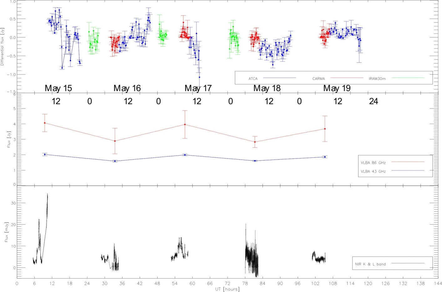
Figure 1: Combined differential light curve of Sgr A* in the mm/sub-mm domain for the May 2007 observing run. The MAMBO 2 bolometer at the IRAM 30 m-telescope was operated at a central wavelength of 1.2 mm (250 GHz). The CARMA data were centred on 100 GHz and the ATCA data on 86 GHz. We also show the daily 7 mm and 3 mm flux density averages from simultaneous VLBA observations (Lu et al. 2008, 2009). In the lower part of the plot, we show the combined NIR light curve consisting of K-band and L’-band light curves (see Appendix for individual light curves). The time axis is labelled with UT hours starting at 00 h on May 15.

We estimate a spectral index variation of $\Delta\alpha=0.07$ between 10¹⁰ Hz and 10¹² Hz from the compilation of radio to sub-mm measurements by Markoff et al. (2001) and Zhao et al. (2003). The maximum spectral range that we cover with CARMA, ATCA, and the IRAM 30 m is 86 GHz to 250 GHz. In total, this gives a maximum expected flux density variation of 8% in the light curve due to spectral index variations between the ATCA, CARMA, and the IRAM 30 m data. The bulk of the data in which we detected the main flux density excursions is covered by the 100 GHz CARMA and the 86 GHz ATCA data. The CARMA and ATCA data follow the VLT data set, while the 30 m data do not detect significant flux density excursions preceding the VLT data. Here the maximum expected flux density variation in the light curve due to spectral index variations can only be 0.005 Jy, which is smaller than $\delta S(t)$. For the CARMA and IRAM 30 m data, the median flux density variation for each epoch (day) is $\delta S(t)\sim 0.1$ Jy, and for the ATCA data we find that $\delta S(t)\sim 0.2$ Jy. These values represent the approximate range in which the datasets can be freely shifted in flux density.
The light curve in Fig. 1 contains two peaks, on May 15 and 17 (there is a weaker, third possible peak on May 19). In Fig. 1, we also show the daily flux density averages of the 7 mm VLBA observations that were conducted in parallel (Lu et al. 2008, 2009; Kunneriath et al. 2008). The VLBA data follow the overall trend of the combined CARMA/ATCA/30 m light-curve very well. The NIR coverage in the K and L’-band is given in the lower panel of Fig. 1 (see Appendix for a description of the scaling and the individual light curves for each day).

To verify the mm/sub-mm flux density variations and in particular the flare detected on 17 May by CARMA, we produced residual maps from the four individual tracks obtained with the CARMA array, since CARMA has the best combination of high resolution and signal-to-noise ratio of all the mm-telescopes we use. These maps shown in Fig. 2 were computed by subtracting the mean of all 4 maps from the maps of individual epochs. The rms noise in these differential maps is of the order of 0.1 Jy per beam. This procedure clearly represents the trend shown in the combined light curve and detects the excess flux density of 0.4 Jy detected on May 17 and a slightly positive flux density on May 19. On the 16th and 18th May 2007, a mixture of negative and positive flux densities in the difference maps corresponds to the non detection of flaring activity in the differential light curve shown in Fig. 1.

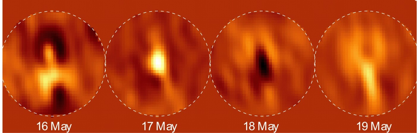
Figure 2: Difference maps at 3 mm of a 40^′′ diameter region (shown by the dashed white line) centred on Sgr A*, obtained from the difference between full synthesis maps of the individual days of CARMA observations and the full CARMA data set as described in the text. The maps have been plotted with the same color-coding table. The figure shows that the flux density variations that are evident from the differential light curves (see Fig. 1) can also be seen in the maps constructed from the corresponding data.

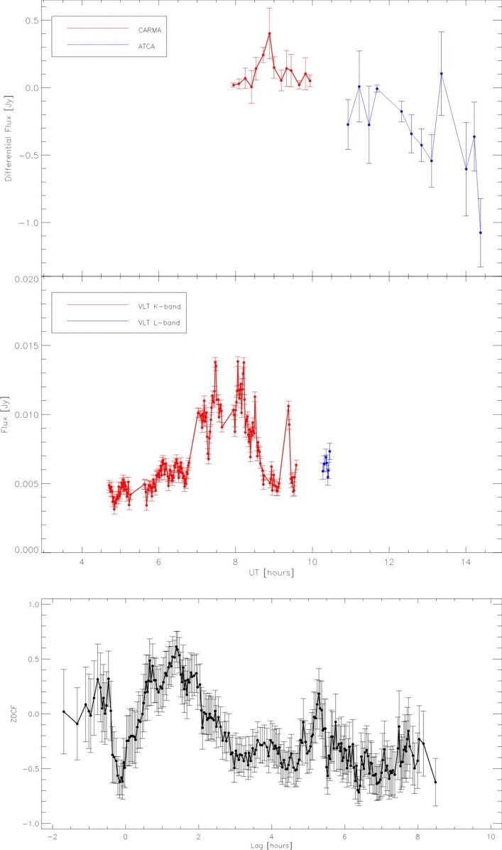
Figure 3: The 3 mm CARMA and ATCA (top red and blue, respectively) and K- and L’-band NIR (middle red and blue, respectively) light curves of the 17 May 2007 flare, with the cross-correlation (bottom) between the two showing that the mm flare follows the NIR flare with a time lag of 1.5$\pm$0.5 hours. ZDCF stands for Z-transformed discrete correlation function.

Figure 4: 3 mm CARMA Sgr A*(top) and calibrator (1733-130) (middle) light curves from 17 May 2007, with the cross-correlation (bottom) between the two showing zero correlation between the calibrator and the source fluxes.

2.2 The NIR data

The NIR data were taken in the K_S-band (2.18 $\mu$m, FWHM 0.35 $\mu$m) and in the L’-band (3.8 $\mu$m, FWHM 0.62 $\mu$m) at ESO’s Very Large Telescope (VLT) with the NACO infrared camera and adaptive optics (AO) system (Rousset et al. 2003; Lenzen et al. 2003) in Chile. For the 3.8 $\mu$m observations, the integration times were NDIT$\times$DIT=200$\times$0.2=40 seconds (DIT is Detector Integration Time, and NDIT is the number of DIT´s). At 2.2 $\mu$m, the integration times were NDIT$\times$DIT=4$\times$10=40 seconds. Additional details of the observation are given in Table 2. The diffraction limit in K-band is about 60 mas. The infrared wavefront sensor of NAOS was used to lock the AO loop on the NIR bright (K-band magnitude $\sim$6.5) supergiant IRS 7, located about $5.6^{\prime\prime}$ north of Sgr A*. Therefore the AO was able to provide a stable correction with a high Strehl ratio (of the order of 50%). After correcting the images for bad pixels, and subtracting the sky and flat fielding, the point spread function (PSF) was extracted from each individual image using $\it{StarFinder}$ (Diolaiti et al. 2000) and a Lucy-Richardson (LR) deconvolution was applied. A Gaussian beam with FWHM corresponding to the respective wavelength ($\sim$60 mas at 2.2 $\mu$m and $\sim$104 mas at 3.8 $\mu$m) was used to restore the beam. To obtain a flux density in Jansky, we perform aperture photometry of the sources with circular apertures of radius 52 mas, apply extinction corrections of A_K=2.8 and A${}_{L^{\prime}}$=1.8, and calibrate the flux with flux densities of known sources, which resulted in K- and L’-band flux densities of S2 of 22$\pm$1 mJy and 9$\pm$1 mJy, respectively. The measurement uncertainties were obtained from the reference star S2.

2.3 Flare events

2.3.1 The 15 May 2007 flare event

The first NIR flare on May 15 detected during the multiwavelength campaign (see also Eckart et al. 2008a) preceded the combined mm/sub-mm monitoring and the first maximum detected therein by nearly 3 hours. The May 15 2007 flare shows 2 polarized bright sub-flares centred on about 07:29 UT and 07:51 UT, respectively, after the start of observations (see Fig. 12 in Appendix). We define sub-flares to be the shorter flux excursions superimposed on the longer main underlying flare. The time difference between the two sub-flares is 22 minutes which is fully consistent with previously reported sub-flare separations. Zamaninasab et al. (2010) demonstrated that these highly polarized sub-flares are part of the flare structure that is significant compared to the randomly polarized red-noise.

The second sub-flare shows substructure that is interpreted by Eckart et al. (2008a) in the framework of spot evolution. The flux density between the 2 sub-flares does not reach the emission level well before and after (i.e., $<$70 and $>$170 minutes into the observations) the flare, probably because of fore- or background stellar flux density contributions (star S17). Additional details of the May 15 2007 NIR flare were given by Eckart et al. (2008a).

For the flux density limit reached in low luminosity states of Sgr A*, the reader is referred to Sabha et al. (2010) and Do et al. (2009). The brief L’-band observations at 10 UT show a NIR signal that is a factor of 2 times stronger than at other times (see Sect. 3.3.1).

2.3.2 The 17 May 2007 flare event

The NIR flare on 17 May had overlap with the CARMA observations, which indicate that a 0.4 Jy 3 mm flare followed the NIR flare.

Figure 3 gives the updated differential light curve obtained from the four longest baselines of CARMA and ATCA, along with the NIR light curve and a cross-correlation between the two showing a time lag of 1.5$\pm$0.5 hours, with a significant, broad and positive peak corresponding to the flares found at both wavelengths. The presence of negative power in the cross-correlation is most likely due to a combination of two effects: (1) The signal-to-noise ratio of the differential ATCA data is lower than that of the CARMA data; and (2) the negative power may also be indicative of residual power on timescales of the length of the (sub-)mm-datasets. Some amount of negative power is expected since we are dealing with differential light curves that measure the variable flux with respect to a median flux level over the length of the corresponding dataset. A significant, broad, and positive cross-correlation peak centred on a time lag of $\sim$1.5 hours is also present if the correlation is only performed with the K-band and CARMA data. Figure 4 shows that the calibrator and source fluxes are not correlated for the CARMA data. Here the cross-correlation was carried out only for the CARMA data since the ATCA array did not observe the same calibrator interleaved with the Sgr A* data.

The NIR K-band data show variable emission, with four sub-flares starting from about 7:00 UT and lasting until the end of the observations at 9:12 UT. The mm-data started at about 8:00 UT and had ended by 10:00 UT. In the mm domain, the variable emission is dominated by a single flare that is slightly wider than the individual NIR sub-flares.

2.3.3 The 19 May 2007 flare event

The flux density excursions on 19 May are only partially constrained by the CARMA millimeter measurements. Two flare events of about 3.5 mJy and 1.1 mJy peak flux density are separated by about 3 hours. The gap in the observations at a time during which the first event reached its peak flux density (see Appendix for individual light curve) implies that the true peak was missed and that the flare was probably brighter than 3.5 mJy. There is an overlap between the NIR and the mm-measurements of about 1.5 hours with no detection of a flare event in the mm-wavelength domain brighter than 0.1-0.2 Jy.

2.3.4 The 26 May 2008 flare event

The 26 May 2008 NIR flare in the L’-band was covered by the CARMA observations, as shown in Fig. 5. The L’-band flare shows a flux density increase of about 70 mJy, followed by a plateau with almost constant flux density at a 40 mJy level. After a total flare duration of 200 minutes, the flux density reaches the original level of 20 mJy. The CARMA data were taken under moderate to poor weather conditions. From 07:10 UT to 11:10 UT, the source visibility was comparable to the levels reached in the 2007 observing session. No flare was detected with a flux density limit of about 0.2 Jy. Starting at 11:10 UT, the weather conditions deteriorated resulting in strong coherence losses.

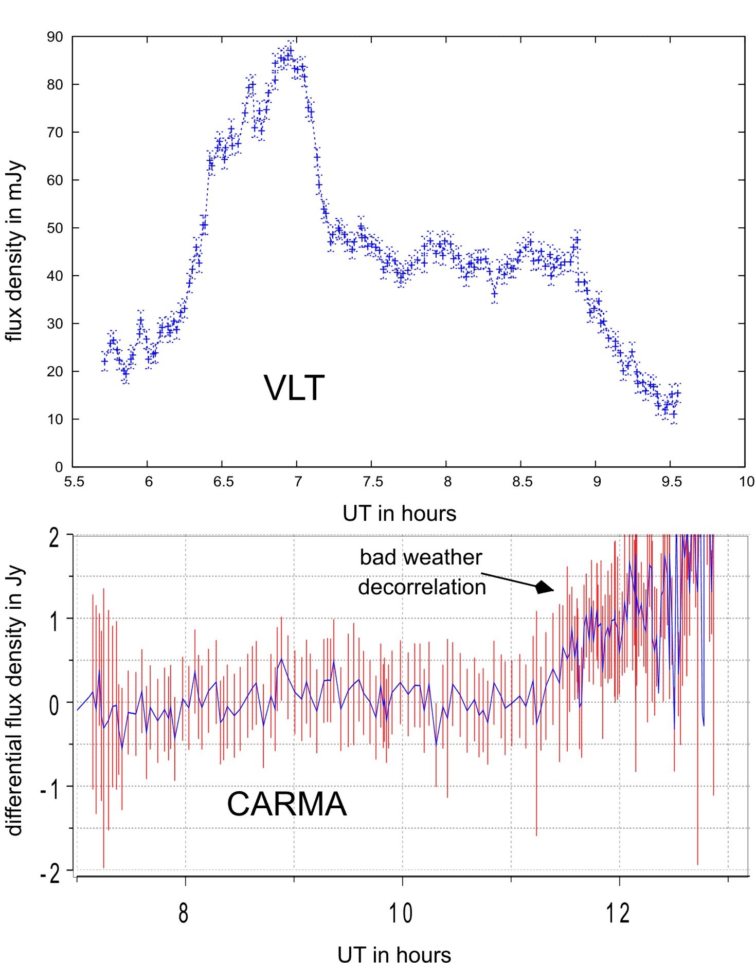
Figure 5: 3.8 $\mu$m NIR flare (top) covered by 3 mm CARMA data (bottom) on the 26 May, 2008. The time coverage of the L’-band flare is from 05:42:55 to 10:37:39 UT.

3 Flare analysis

The seven coordinated Sgr A* measurements reported so far that include sub-mm/mm data (Eckart et al. 2006a, 2008b; Yusef-Zadeh et al. 2006b; Marrone et al. 2008; Yusef-Zadeh et al. 2009, including this work) have shown that the observed sub-millimeter/mm flares follow the largest event observed at shorter wavelengths (NIR/X-ray; see detailed discussion in Marrone et al. (2008)) with a delay of $\sim$1.5$\pm$0.5 hours. We therefore assume that the millimeter flares presented here are related to the observed IR flare events. This flaring activity can be explained using a multi-component relativistic spot/disk model and an adiabatic expansion model in combination with a synchrotron self Compton (SSC) formalism. While this model has been presented before (see references above), it is essential to test new datasets against it to improve our understanding of the variable emission from Sgr A*.

3.1 Relativistic spot/disk modelling of NIR flares

Multiple hot spots revolving around a black hole in an accretion disk in AGNs or galactic black holes can give rise to light curves in the X-ray and NIR regimes whose power spectral density (PSD) is described by a broken power law with a slope similar to that of red noise processes (Armitage & Reynolds 2003; Pecháček et al. 2008; Do et al. 2008). Simulations show that polarized light curves exhibit behaviour associated with lensing of hot spots orbiting around a SMBH (Zamaninasab et al. 2010). Previously observed NIR light curves of Sgr A* have been successfully modelled by a multi-component hot spot model involving source components orbiting around the SMBH in a temporary accretion disk (Eckart et al. 2006b; Meyer et al. 2006b, a, 2007; Zamaninasab et al. 2008b, a).

This relativistic model consists of source components that are a mix of synchrotron and SSC components with an optically thin spectral index $\alpha$ and relativistic electrons with $\gamma$_e$\sim$10³, using the formalism described by Gould (1979) and Marscher (1983). The KY-code by Dovčiak et al. (2004) produces light amplification curves for each individual component orbiting the SMBH taking into account relativistic effects, and by combining these curves with the SSC model, we can estimate the SSC X-ray and NIR flux densities and the magnetic field (Eckart et al. 2008a). Figure 6 presents simulations of the accretion disk with multiple spots revolving around the SMBH, and Fig. 7 gives the light curves produced by these simulations. Zamaninasab et al. (2010) describe the modelling and simulations shown in Figs. 6 and 7 in greater detail.

These light curves may be the result of a single hot spot that dominates the disk for several orbital periods. If the spot were to sink (as may occur) towards the centre while orbiting, this would cause a quasi-periodic modulation of the light curve for the time the emission of the spot dominates the red-noise emission of the remaining disk. This modulation may also be produced by several different hot spots that have individual lifetimes of shorter than one orbital period close to the last stable orbit. In this case, the light-curve will be modulated quasi-periodically at a rate close to the frequency of the last stable orbit (see discussion in Eckart et al. 2008a and Eckart et al. 2006b). If the hot spots expand within the accretion disk or are the source of a short outflow above the disk, this quasi-periodic signal will be smeared out. In particular, it may be undetectable at lower (sub-)mm observing frequencies (see below). In the case of our experiment, only the NIR data on 15 May shows a strong sub-flare modulation (as explained below) that may be linked to quasi-periodicity. All other NIR flares (with the possible exception of the steeply rising and falling flanks of the L’-band flare on 26 May 2008) cannot be associated with this phenomenon. However, in the case of a source expansion this model can be linked to the adiabatic expansion model for synchrotron sources that is described in the following section.

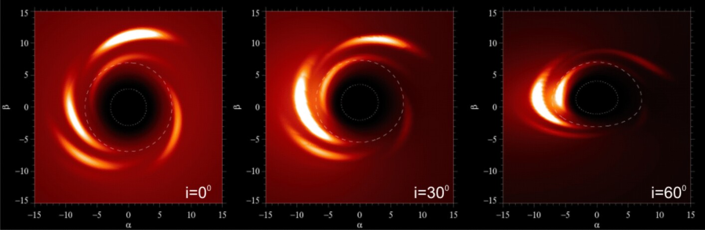
Figure 6: Simulated images of multiple spots revolving around a black hole, projected on the observer image plane ($\alpha$, $\beta$), viewed at three inclination angles i=0⁰, 30⁰, and 60⁰, with respect to the common rotation axis. The dotted and dashed circles represent the event horizon and the marginally stable orbit, respectively.

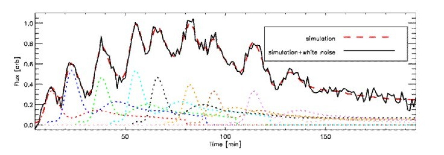
Figure 7: Light curve obtained from the multiple spot simulations shown in Fig. 6, the solid black line representing the overall light curve and the different coloured dashed lines showing the contributions of individual spots.

3.2 Adiabatically expanding source components

Adiabatic expansion of the synchrotron components can explain the apparent time difference of 1.5$\pm$0.5 hours between the NIR and sub-mm/mm flares (Eckart et al. 2006a, 2008b; Yusef-Zadeh et al. 2006a). We assume a uniformly expanding blob of relativistic electrons with a power-law energy spectrum, $n(E)\propto E^{-p}$, threaded by a magnetic field that declines as $R^{-2}$, and of energy and density that decline as $R^{-1}$ and $R^{-3}$, respectively, as a result of expansion of the blob (van der Laan 1966). If $R_{0}$, $S_{0}$ and $\tau$₀ are the size, flux density, and optical depth of the source component at the peak frequency ($\nu$₀) of the synchrotron spectrum, the optical depth and flux density at a given frequency $\nu$ scale as

$$\tau_{\nu}=\tau_{0}\left(\frac{\nu}{\nu_{0}}\right)^{-(p+4)/2}\left(\frac{R}{R_{0}}\right)^{-(2p+3)}$$ (8)

and

$$S_{\nu}=S_{0}\left(\frac{\nu}{\nu_{0}}\right)^{5/2}\left(\frac{R}{R_{0}}\right)^{3}\frac{1-\exp(-\tau_{\nu})}{1-\exp(-\tau_{0})},$$ (9)

respectively. Here $\tau$₀ is defined to be the optical depth corresponding to the frequency at which the flux density is maximum, in accordance with van der Laan’s model (1966), to be able to combine the SSC formalism with an adiabatic expansion model.This makes $\tau$₀ dependent only on $p$ through the condition

$$e^{\tau_{0}}-\tau_{0}(p+4)/5-1=0.$$ (10)

For instance, if $p$ ranges from 1 to 3, $\tau$₀ ranges from 0 to 0.65. Thus for a given particle spectral index $p$ and peak flux density $S_{0}$ at a frequency $\nu$₀, the model gives the variation in flux density at any frequency as a function of the expansion factor $(R/R_{0})$. To convert the dependence on radius to a dependence on time, we assume a simple linear expansion model with a constant expansion speed of $v_{\mathrm{exp}}$, such that $R$-$R$₀=v_exp($t$-$t_{0}$). At times $t$$<$$t_{0}$, we assume that the source has an optical depth equal to its frequency-dependent initial value $\tau$₀ at $R$=$R_{0}$. For the optically thin part of the spectrum, the flux increases initially with increasing source size at constant optical depth $\tau$₀ and then decreases with decreasing optical depth as it expands. One Schwarzschild radius corresponds to $R_{s}$=2$GM$/$c$²$\sim$10¹⁰ m for a $\sim$4$\times$10⁶ M_⊙ supermassive black hole, which infers the velocity of light to be about 100$R_{s}$ per hour. For $t$$>$$t_{0}$, increasing the turnover frequency $\nu$₀ or initial source size $R_{0}$ has the effect of shifting the decaying flank of the curve to later times, as does decreasing the spectral index $\alpha_{\mathrm{synch}}$ or peak flux density $S_{0}$. Increasing the adiabatic expansion velocity v_exp, on the other hand, shifts the peak of the light curve to earlier times. Flare timescales are longer at lower frequencies and have a slower decay rate, as a result of adiabatic expansion.

date	model	source	$\Delta$$t$	$v_{\mathrm{exp}}$	$S_{\mathrm{max,obs}}$	$\alpha_{\mathrm{synch}}$	$R_{0}$	$\nu_{\mathrm{max,obs}}$	$B$	$S_{\mathrm{NIR,synch}}$	$S_{\mathrm{NIR,SSC}}$	$S_{\mathrm{X-ray,SSC}}$
	label		hours	in $c$	[Jy]		[Rs]	[GHz]	[G]	[mJy]	[mJy]	[nJy]
$1\leavevmode\nobreak\ \sigma$ $\rightarrow$			$\pm$1.0	$\pm$0.001	$\pm$0.1	$\pm$0.1	$\pm$0.1	$\pm$250	$\pm$10	$\pm$1.0	$\pm$1.0	$\pm$20
15 May 2007	A	$\alpha$	0.0	0.007	0.6	0.85	1.3	340	33	3.1	$<$0.03	$<$10
		$\beta$	0.0		0.3	0.60	0.3	840	29	12	$<$0.03	$<$10
		$\gamma$	0.30		0.3	0.75	0.2	840	32	5.6	$<$0.03	$<$10
15 May 2007	B	$\alpha$	0.0	0.017	0.6	0.65	1.3	340	37	8.3	$<$0.02	$<$40
		$\beta$	0.0		0.3	0.65	0.3	840	30	8.4	$<$0.02	$<$40
		$\gamma$	0.37		0.3	0.65	0.35	810	32	8.4	$<$0.02	$<$40
17 May 2007	A	$\alpha$	0.0	0.010	1.0	1.00	0.8	840	66	4.7	$<$0.01	$<$10
		$\beta$	0.45		0.5	0.97	0.3	1250	66	4.0	$<$0.01	15
		$\gamma$	-0.59		1.3	1.11	1.0	840	69	3.2	$<$0.01	$<$10
		$\delta$	-0.96		0.5	1.02	0.3	1250	68	3.2	$<$0.01	12
17 May 2007	B	$\alpha$	0.0	0.011	0.25	0.70	0.2	1360	86	8.1	$<$0.01	19
		$\beta$	0.36		0.25	0.70	0.2	1360	86	8.1	$<$0.01	19
		$\gamma$	-0.69		0.17	0.70	0.2	1360	65	5.1	$<$0.01	21
		$\delta$	-1.05		0.17	0.70	0.2	1360	65	5.1	$<$0.01	21
		$\epsilon$	-0.33		1.75	1.05	1.6	570	68	7.1	$<$0.01	$<$2
19 May 2007	A	$\alpha$	0.0	0.007	1.30	1.07	1.0	1360	67	3.5	$<$0.01	$<$10
		$\beta$	2.50		1.10	1.10	0.8	1360	67	0.5	$<$0.01	$<$10
		$\gamma$	2.90		1.10	1.10	0.8	1360	67	0.5	$<$0.01	$<$10
19 May 2007	B	$\alpha$	0.0	0.017	1.33	1.13	1.0	720	68	2.5	$<$0.01	$<$10
		$\beta$	0.50		1.33	1.09	1.0	720	67	3.1	$<$0.01	$<$10
		$\gamma$	2.85		1.50	1.30	0.8	820	72	1.2	$<$0.02	$<$10
		$\delta$	3.30		1.50	1.30	0.8	850	72	1.2	$<$0.02	$<$10
26 May 2008	A	$\alpha$	0.0	0.005	1.1	0.68	0.5	1090	30	31	$<$0.02	41
		$\beta$	-0.45		1.0	0.68	0.5	1090	40	26	$<$0.02	18
		$\gamma$	0.52		1.0	0.83	0.5	1030	31	15	$<$0.02	17
		$\delta$	1.03		1.0	0.80	0.5	1160	34	17	$<$0.03	23
		$\epsilon$	1.48		0.8	0.77	0.5	1160	48	16	$<$0.01	$<$10
		$\zeta$	1.90		0.8	0.77	0.5	1160	48	16	$<$0.01	$<$10
26 May 2008	B	$\alpha$	0.0	0.007	1.4	0.70	0.6	1090	44	39	$<$0.02	24
		$\beta$	-0.40		1.3	0.70	0.6	1090	56	35	$<$0.02	13
		$\gamma$	0.52		1.1	0.77	0.6	1030	36	23	$<$0.02	18
		$\delta$	1.03		1.3	0.80	0.5	1160	33	23	$<$0.04	33
		$\epsilon$	1.48		1.0	0.77	0.5	1160	58	20	$<$0.01	$<$10
		$\zeta$	1.90		1.0	0.73	0.5	1160	56	24	$<$0.01	$<$10

Table 3: Source component parameters for the combined SSC and adiabatic expansion model of the 15, 17, and 19 May 2007 and the 26 May 2008 flares. Labels A and B refer to models with lower and higher expansion velocities, respectively. The flare times $\Delta$$t$ are given with respect to the peak of the brighter NIR flares. In addition to $v_{\mathrm{exp}}$, the $R_{0}$ values are responsible for the position and width of the infrared flare peaks in time. Different values for $\alpha_{\mathrm{synch}}$ are required to match the infrared flux densities.

3.3 Adiabatic expansion modelling

Table 3 summarises the properties of the model, such as the adiabatic expansion velocity $v_{\mathrm{exp}}$, the optically thin spectral index $\alpha$_synch, cutoff frequency $\nu$_max,obs, and flux density $S$_max,obs of the source components, using the same nomenclature as Eckart et al. (2006a, 2009). The optically thin NIR flux density is represented by $S$_NIR,synch, while $S$_NIR,SSC and $S$_X-ray,SSC give the upper limits to the flux densities of upscattered SSC components. A global variation in a single parameter by the value listed in the corresponding column in Table 3 results in an increase of $\Delta\chi=1$ (from the reduced $\chi^{2}$ value). Here global variation means adding to a single model parameter for all source components the 1$\sigma$ uncertainty, such that a maximum positive or negative flux density deviation is reached. Alternatively, a variation by the listed uncertainty for only a single source component results in a variation of the model predicted NIR and X-ray flux density by more than 30%. Judging from the $\Delta\chi$ based on the mm-data alone, the global uncertainties for $S_{\mathrm{max,obs}}$, $\alpha_{\mathrm{synch}}$, and $R_{0}$ may then be doubled.
When performing the reduced $\chi^{2}$ fit for $N$ source components, we used $N$ times 4 ($S_{\mathrm{max,obs}}$, $\alpha_{\mathrm{synch}}$, $R_{0}$, $\nu_{\mathrm{{max}}}$) plus one common expansion velocity $v_{\mathrm{exp}}$ and time offset (leaving the time differences between the components fixed), i.e., 4$N$+2 degrees of freedom. Unfortunately, the model parameters may not all be considered independent, e.g., the width and peak of a light curve signature depends to a varying extent on all 4 parameters $S_{\mathrm{max}}$, $\alpha_{\mathrm{synch}}$, $R_{0}$, and $\nu_{\mathrm{max}}$. Therefore, for all models we stayed with the minimum number of source components to estimate the degrees of freedom. Since in the case of the May 2007 flare the VLT data consist of $\sim$10 times the number of CARMA data points, we weighted the squared CARMA flux deviations and number of data points by an additional factor of 19. The $\chi^{2}$ test was then carried out using the sum of the squared flux deviations and data points of the VLT and CARMA datasets.
In general, we aimed to develop a model at a lower and a higher expansion speed labelled A and B (Table 3). In comparison to earlier modelling results (Eckart et al. 2008a, 2009; Yusef-Zadeh et al. 2008; Marrone et al. 2008), these speeds were chosen to be 0.007$c$ and 0.017$c$ for the 15 May and 19 May 2007 flares. For the 17 May 2007 and the 26 May 2008 data, a violation of the observed flare width and the expected range for the magnetic field strength restricted the choice of expansion speeds. For comparison, we listed the model components in Table 3. The models were developed by minimizing the number of free parameters (and maximizing the description of significant flare features in the observed light curves).

SSC modelling as an additional constraint: The SSC model described in Sect. 3.1 allows us to estimate the SSC contribution of the X-ray and NIR flux densities, and the magnetic field. Higher SSC NIR emission would violate the assumption in our adiabatic expansion model that the dominant source of NIR flux density is synchrotron emission of the THz peaked expanding component, as well as require us to model the unknown X-ray flux density. Magnetic fields of up to $\sim$70 gauss (Eckart et al. 2006a, 2008b; Yusef-Zadeh et al. 2008; Marrone et al. 2008) have been obtained for previous models via $B\sim\theta^{4}\nu_{m}^{5}S_{m}^{-2}$, where $\nu$_m and S_m are the synchrotron turnover frequency and flux density, respectively. These results should also not be violated by the model.
The expansion speed: The model yields expansion velocities from 0.005$c$ - 0.017$c$ (see Table 3), which agree well with previously published results (Yusef-Zadeh et al. 2008). These velocities are lower than expected for relativistic sound speed in orbital velocity near the SMBH. This may be caused by the bulk velocity of the source components being larger than the expansion velocity $v_{\mathrm{exp}}$ or because the expanding material is confined to the immediate region surrounding Sgr A* in the form of a disk or corona. In this case, shearing caused by differential rotation within the accretion disk is responsible for the ’expansion’ and the observed low expansion velocities (Eckart et al. 2008b; Zamaninasab et al. 2008b; Pecháček et al. 2008). Owing to the expansion or the presence of several strong spots in the disk or corona, the short time modulation often seen in the NIR will also be smeared out in the (sub-)mm-wavelength domain - implying that it may not be observable at all at these wavelengths.
By comparing other flare events that were detected simultaneously at X-ray and sub-mm/mm-wavelengths, we imposed the additional constraint that the 100 GHz flux density should not be much stronger than about 0.2 Jy, 1.5$\pm$0.5 hours after the NIR event, and the X-ray flux density should be limited to a few 10 nJy. The following sections describe the modelling of the individual flares.

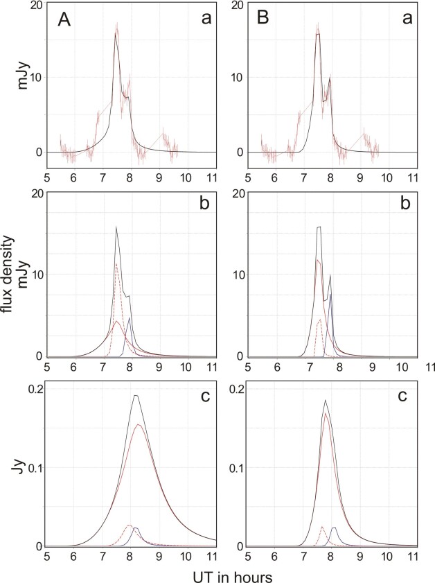
Figure 8: Models A and B of the 15 May 2007 NIR flare: a) Fitted NIR light curve, with the black curve corresponding to the model and the red curve corresponding to the data, b) Contribution of individual source components to NIR light curve, and c) Contribution of individual source components to mm light curve.

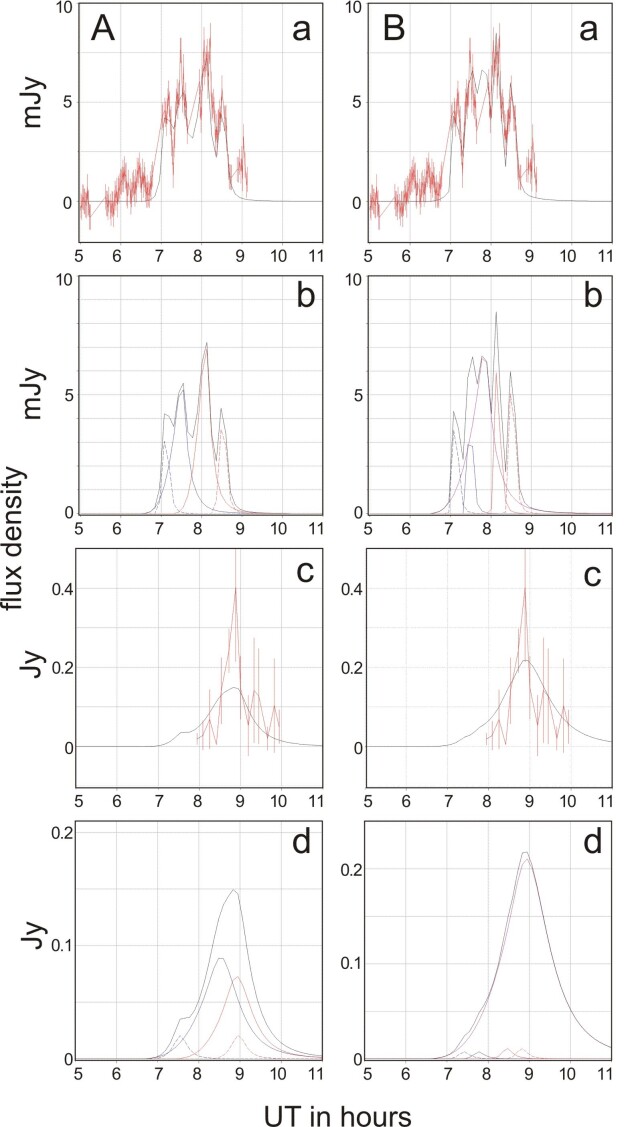
Figure 9: Models A and B of the 17 May 2007 NIR flare: a) Fitted NIR light curve, with the black curve corresponding to the model and the red curve corresponding to the data, b) Contribution of individual source components to NIR light curve, c) Fitted mm light curve, with the black curve corresponding to the model and the red curve corresponding to the data, and d) Contribution of individual source components to mm light curve.

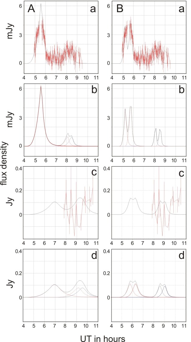
Figure 10: Models A and B of the 19 May 2007 NIR flare: a) Fitted NIR light curve, with the black curve corresponding to the model and the red curve corresponding to the data, b) Contribution of individual source components to NIR light curve, c) Fitted mm light curve, with the black curve corresponding to the model and the red curve corresponding to the data, and d) Contribution of individual source components to mm light curve.

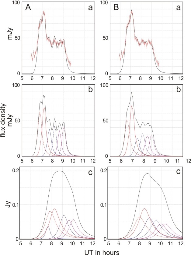
Figure 11: Models A and B of the 26 May 2008 NIR flare: a) Fitted NIR light curve, with the black curve corresponding to the model and the red curve corresponding to the data, b) Contribution of different source components to NIR light curve, and c) Contribution of different source components to mm light curve.

3.3.1 Expansion modelling of the 15 May flare emission

The 15 May 2007 flare can only be constrained by means of its NIR lightcurve (Fig. 8) since the mm data begins nearly 3 hours after the first peak in the NIR. According to the adiabatic expansion model, 3-4 hours after the NIR flare, the flux density in the mm band was insufficiently strong to be significant compared to the median flux density variations in the data. We modelled a background component $\beta$ and two components for the two strongest sub-flares $\alpha$ and $\gamma$. The expansion speed could not be constrained at all. In model A, we used a value of 0.007$c$, close to the speed we found for most of the modelled flares. In model B, we used a higher speed of 0.017$c$, which required lower spectral indices and a weaker background component to obtain a good fit to the NIR data and to fullfil the upper limits at 100 GHz and in the X-ray domain.

A correlation between the L’-band data at 10 UT and the radio data cannot be excluded, but the L’-band data light curve is not long enough to justify including this data in a full modelling of the NIR/mm-light curves in the framework of the adiabatic expansion model. However, high NIR flux density levels precede a positive flux density excursion in the mm-domain, as it is expected to in the framework of the adiabatic expansion model. Although the L’-band flux density is higher than that at other times, the event is not linked to a particularly strong flux density excursion in the mm-domain. However, the high L’-band flux may also be caused by a transient steeper infrared spectral index. This may indicate either a significantly higher turnover frequency (extrapolating into the sub-mm domain) or the presence of stronger synchrotron losses. Both effects may explain a lack of strong mm-emission following the NIR event at 10 UT.

3.3.2 Expansion modelling of the 17 May flare emission

The 17 May 2007 flare is constrained by the NIR and CARMA mm-data (Fig. 9). This time lag of 1.5$\pm$0.5 hours between the flare events mainly determines the expansion velocity. A constant flux density of 0.003 Jy was subtracted from the NIR data to model the individual flare events. We present two modelling approaches that lead to a successful description of the flare. In model A, we used only 4 components describing 4 sub-flares $\alpha$ through $\delta$. Motivated by the relativistic disk modelling referred to in Sect. 3.1, we used in model B a background component $\epsilon$ located close to the centre of the overall NIR flare. We then modelled the 4 sub-flares with additional components. In comparison to model A, this results in lower values for $S_{\mathrm{max,obs}}$ and the spectral index $\alpha_{\mathrm{synch}}$, smaller source component sizes $R_{0}$, and higher cutoff frequencies $\nu_{\mathrm{max,obs}}$ for components $\alpha$ through $\delta$. The quality of the fit is comparable for models A and B.

3.3.3 Expansion modelling of the 19 May flare emission

For the 19 May 2007 flare, the slower adiabatic expansion velocity of 0.007$c$ allows us to fit the first event (centred on the NIR at $\sim$5:30 UT) with a single component (Fig. 10). For higher velocities, a larger number of source components has to be used to model the NIR data. For both velocities, the second, later flare component (centred on the NIR at $\sim$8:20 UT) is constrained by the 3 mm CARMA data. For the model parameters used to match the NIR data, the predicted 3 mm flux densities of both flare components (at $\sim$5:30 UT and $\sim$8:20 UT) are at or below the flux density limit of 0.1-0.2 Jy, above which no millimeter wavelength flare event has been detected.

3.3.4 Expansion modelling of the 26 May flare emission

Modelling the 26 May 2008 flare (Fig. 11) requires a satisfactory description of an initially bright flare with sharply rising and falling flanks followed by a 1.5 hour plateau. This can only be achieved with several source components each covering a maximum portion of time of about a 30 minute duration. A smaller number of source components would require larger source component sizes resulting in higher magnetic fields and a violation of the 100 GHz flux limit. Given these difficulties, the number of source components is of course not unique and the models proposed in Table 3 can only be taken as an example.

The overall flare structure is quite reminiscent of the flare that was observed on 3 June 2008 simultaneously using APEX and the VLT, as described by Eckart et al. (2008b), with the exception that the 26 May flare is more continuous than the 3 June 2008 flare. An overall flare structure that starts out with a bright event followed by a single or a few fainter events was also reported by Eckart et al. (2006a, 2009). These events may relate to a common physical structure. An explanation could be a disk structure that is expanded by differential rotation within the disk. Alternative explanations may involve a common history in terms of either accretion or magnetic field instability - possibly also within a jet structure (see Eckart et al. (2008b, a) and Sect. 4).

4 Alternative short jet model

Emission from a jet and an underlying accretion process may also account for the spectrum of Sgr A*, with the plasma in the jet starting to become optically thin at longer wavelengths with increasing distance from the centre. Thus, radiation at different radio wavelengths probe different sections of the jet, leading to a correlation with emission in other wavelength regimes. Very close to the SMBH, it is difficult to distinguish between emission from the jet and the accretion flow. For this jet model, flux variations may then be caused by accretion processes or jet instabilities rather than be the result of modulation from an orbiting spot, followed by an adiabatic expansion of jet components. Details of a compact, weak jet structure are discussed in Markoff et al. (2007) (also Markoff et al. 2005).

5 Summary

We have presented results from global coordinated multiwavelength observational campaigns carried out in 2007 and 2008 using NACO at VLT in the NIR K- and L’-bands, and CARMA, ATCA, and IRAM in the mm regime.

We have presented a new method to obtain concatenated light curves of the compact mm-source Sgr A* from single dish telescopes and interferometers in the presence of significant flux density contributions from an extended and only partially resolved source. The method requires several consecutive datasets to be available for each participating observatory. From these data, we have evidence of four different flaring events in the NIR, with three of these events being covered later in the mm regime.

We have modelled the flare emission with a model involving adiabatic expansion of synchrotron source components, and obtained spectral index values, expansion velocities, and other parameters that are consistent with previously published variability studies. The mm-flares were found to occur on average about 1.5$\pm$0.5 hours after the NIR flare emission, and the expansion velocities for the various flares ranged from 0.005$c$ - 0.017$c$.

Modelling the NIR-flares with synchrotron components that become optically thick in the sub-mm wavelength regime and obey the flux density values or limits in the mm- and X-ray domain constrains their turnover frequency and flux density. For the described global experiment, the low mm-regime flux density limits imply that the turnover frequencies are not lower than about 1.0$\pm$0.3 THz and that the optically thick peak flux densities at or below this turnover frequencies do not exceed about $\sim$1 Jy on average. However, in other experiments the source showed higher flux density flare emission in the mm-domain (e.g., 0.5-1.5 Jy in the sub-mm; Yusef-Zadeh et al. 2009, Marrone et al. 2008, Eckart et al. 2008, 2006b)

Further monitoring of the variability of Sgr A* in different wavelength regimes (including X-ray, NIR, sub-mm, and mm radio) and in polarised NIR/radio emission is required to improve our understanding of the adiabatic expansion model and improve statistics describing the flaring activity. Current mm-interferometers such as CARMA, PdBI, and ATCA and future telescopes such as ALMA which are able to distinguish between emission from Sgr A* and the thermal emission of the CND and mini-spiral surrounding the SMBH, and NIR telescopes with large apertures such as VLT, Keck, and LBT, which can distinguish Sgr A* from surrounding stars, may be combined to provide us with high quality data to study the evolution of synchrotron components in greater detail. With future mm-VLBI measurements at frequencies of 230 GHz and above, imaging of the central region of Sgr A* may become possible, enabling a deeper study of the accretion physics and testing of current theories of emission in the region (Doeleman et al. 2008, 2009).

Appendix:NIR light curves

The individual NIR K and L’-band light curves from Fig. 1 are shown in Figs. 12 to 16. A spectral index of -0.9 (as we preferentially used in our modelling, see Table 3 and Eckart et al. 2008b, 2009, Yusef-Zadeh et al. 2008) gives us a scaling factor of 0.6, which we use to scale the L’-band data, and then combine the K and L’-band data as shown in Fig. 1 and Figs. 12 to 16. In the remaining figures, no scaling has been applied. The uncertainties in flux measurements were obtained from the reference star S2, which has known flux densities of 22$\pm$1 mJy and 9$\pm$1 mJy in the K and L’-bands, respectively.

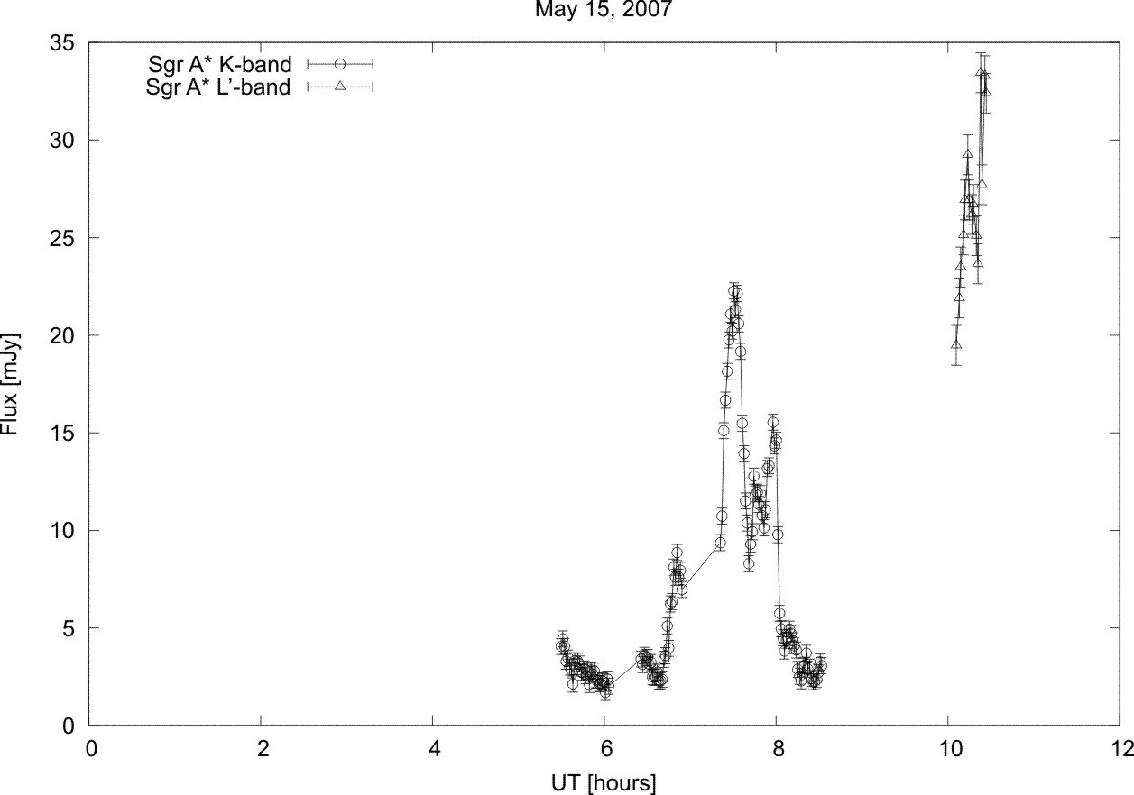
Figure 12: Observing time–K-band: 05:29:55 to 08:31:48, L’-band: 10:05:48 to 10:26:45

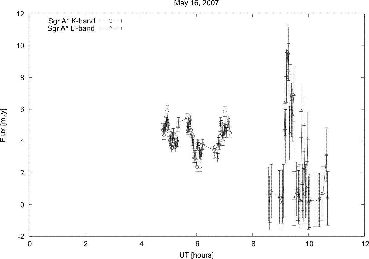
Figure 13: Observing time–K-band: 04:47:22 to 07:54:41, L’-band: 08:34:27 to 10:41:46

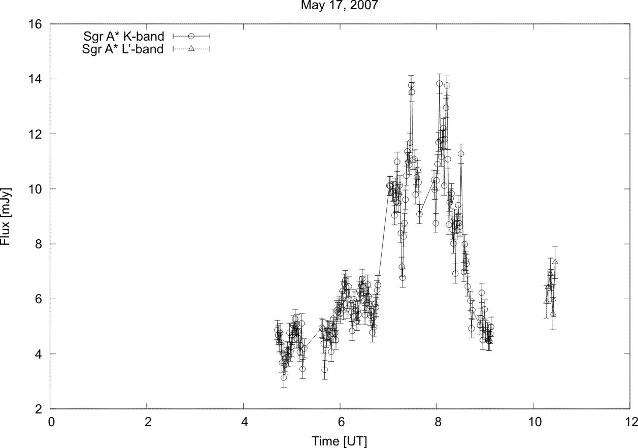
Figure 14: Observing time–K-band: 04:42:14 to 09:34:40, L’-band: 10:16:24 to 10:27:06

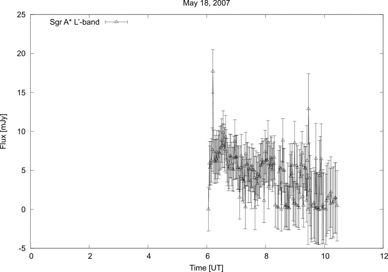
Figure 15: Observing time–L’-band: 06:03:26 to 10:26:00

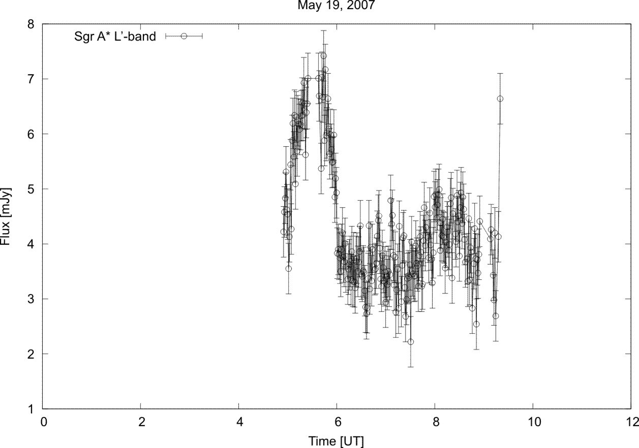
Figure 16: Observing time–K-band: 04:55:00 to 09:28:22

References

- Armitage & Reynolds (2003) Armitage, P. J. & Reynolds, C. S. 2003, MNRAS, 341, 1041
- Bock et al. (2006) Bock, D., Bolatto, A. D., Hawkins, D. W., et al. 2006, in Society of Photo-Optical Instrumentation Engineers (SPIE) Conference Series, Vol. 6267, Society of Photo-Optical Instrumentation Engineers (SPIE) Conference Series
- Bower et al. (2002) Bower, G. C., Falcke, H., Sault, R. J., & Backer, D. C. 2002, ApJ, 571, 843
- Christopher et al. (2005) Christopher, M. H., Scoville, N. Z., Stolovy, S. R., & Yun, M. S. 2005, ApJ, 622, 346
- Diolaiti et al. (2000) Diolaiti, E., Bendinelli, O., Bonaccini, D., et al. 2000, in Society of Photo-Optical Instrumentation Engineers (SPIE) Conference Series, Vol. 4007, Society of Photo-Optical Instrumentation Engineers (SPIE) Conference Series, ed. P. L. Wizinowich, 879–888
- Do et al. (2008) Do, T., Ghez, A. M., Morris, M. R., et al. 2008, Journal of Physics Conference Series, 131, 012003
- Do et al. (2009) Do, T., Ghez, A. M., Morris, M. R., et al. 2009, ApJ, 691, 1021
- Doeleman et al. (2009) Doeleman, S. S., Fish, V. L., Broderick, A. E., Loeb, A., & Rogers, A. E. E. 2009, ApJ, 695, 59
- Doeleman et al. (2008) Doeleman, S. S., Weintroub, J., Rogers, A. E. E., et al. 2008, Nature, 455, 78
- Dovčiak et al. (2004) Dovčiak, M., Karas, V., & Yaqoob, T. 2004, ApJS, 153, 205
- Eckart et al. (2004) Eckart, A., Baganoff, F. K., Morris, M., et al. 2004, A&A, 427, 1
- Eckart et al. (2009) Eckart, A., Baganoff, F. K., Morris, M. R., et al. 2009, A&A, 500, 935
- Eckart et al. (2006a) Eckart, A., Baganoff, F. K., Schödel, R., et al. 2006a, A&A, 450, 535
- Eckart et al. (2008a) Eckart, A., Baganoff, F. K., Zamaninasab, M., et al. 2008a, A&A, 479, 625
- Eckart & Genzel (1996) Eckart, A. & Genzel, R. 1996, Nature, 383, 415
- Eckart et al. (2002) Eckart, A., Genzel, R., Ott, T., & Schödel, R. 2002, MNRAS, 331, 917
- Eckart et al. (2008b) Eckart, A., Schödel, R., García-Marín, M., et al. 2008b, A&A, 492, 337
- Eckart et al. (2006b) Eckart, A., Schödel, R., Meyer, L., et al. 2006b, A&A, 455, 1
- Eisenhauer et al. (2005) Eisenhauer, F., Genzel, R., Alexander, T., et al. 2005, ApJ, 628, 246
- Eisenhauer et al. (2003) Eisenhauer, F., Schödel, R., Genzel, R., et al. 2003, ApJ, 597, L121
- Genzel et al. (1997) Genzel, R., Eckart, A., Ott, T., & Eisenhauer, F. 1997, MNRAS, 291, 219
- Genzel et al. (2000) Genzel, R., Pichon, C., Eckart, A., Gerhard, O. E., & Ott, T. 2000, MNRAS, 317, 348
- Ghez et al. (2009) Ghez, A., Morris, M., Lu, J., et al. 2009, in Astronomy, Vol. 2010, AGB Stars and Related Phenomenastro2010: The Astronomy and Astrophysics Decadal Survey, 89–+
- Ghez et al. (2004a) Ghez, A. M., Hornstein, S. D., Bouchez, A., et al. 2004a, in Bulletin of the American Astronomical Society, Vol. 36, Bulletin of the American Astronomical Society, 1384–+
- Ghez et al. (1998) Ghez, A. M., Klein, B. L., Morris, M., & Becklin, E. E. 1998, ApJ, 509, 678
- Ghez et al. (2000) Ghez, A. M., Morris, M., Becklin, E. E., Tanner, A., & Kremenek, T. 2000, Nature, 407, 349
- Ghez et al. (2005) Ghez, A. M., Salim, S., Hornstein, S. D., et al. 2005, ApJ, 620, 744
- Ghez et al. (2004b) Ghez, A. M., Wright, S. A., Matthews, K., et al. 2004b, ApJ, 601, L159
- Gillessen et al. (2009) Gillessen, S., Eisenhauer, F., Trippe, S., et al. 2009, ApJ, 692, 1075
- Gould (1979) Gould, R. J. 1979, A&A, 76, 306
- Guesten et al. (1987) Guesten, R., Genzel, R., Wright, M. C. H., et al. 1987, ApJ, 318, 124
- Herrnstein et al. (2004) Herrnstein, R. M., Zhao, J., Bower, G. C., & Goss, W. M. 2004, AJ, 127, 3399
- Kunneriath et al. (2008) Kunneriath, D., Eckart, A., Vogel, S., et al. 2008, Journal of Physics Conference Series, 131, 012006
- Lenzen et al. (2003) Lenzen, R., Hartung, M., Brandner, W., et al. 2003, in Society of Photo-Optical Instrumentation Engineers (SPIE) Conference Series, Vol. 4841, Society of Photo-Optical Instrumentation Engineers (SPIE) Conference Series, ed. M. Iye & A. F. M. Moorwood, 944–952
- Lu et al. (2008) Lu, R., Krichbaum, T. P., Eckart, A., et al. 2008, Journal of Physics Conference Series, 131, 012059
- Lu et al. (2009) Lu, R., Krichbaum, T. P., Eckart, A., et al. 2009, A&A, in prep.
- Markoff et al. (2007) Markoff, S., Bower, G. C., & Falcke, H. 2007, MNRAS, 379, 1519
- Markoff et al. (2001) Markoff, S., Falcke, H., Yuan, F., & Biermann, P. L. 2001, A&A, 379, L13
- Markoff et al. (2005) Markoff, S., Nowak, M. A., & Wilms, J. 2005, ApJ, 635, 1203
- Marrone et al. (2008) Marrone, D. P., Baganoff, F. K., Morris, M. R., et al. 2008, ApJ, 682, 373
- Marscher (1983) Marscher, A. P. 1983, ApJ, 264, 296
- Mauerhan et al. (2005) Mauerhan, J. C., Morris, M., Walter, F., & Baganoff, F. K. 2005, ApJ, 623, L25
- Meyer et al. (2006a) Meyer, L., Eckart, A., Schödel, R., et al. 2006a, A&A, 460, 15
- Meyer et al. (2007) Meyer, L., Schödel, R., Eckart, A., et al. 2007, A&A, 473, 707
- Meyer et al. (2006b) Meyer, L., Schödel, R., Eckart, A., et al. 2006b, A&A, 458, L25
- Pecháček et al. (2008) Pecháček, T., Karas, V., & Czerny, B. 2008, A&A, 487, 815
- Rousset et al. (2003) Rousset, G., Lacombe, F., Puget, P., et al. 2003, in Society of Photo-Optical Instrumentation Engineers (SPIE) Conference Series, Vol. 4839, Society of Photo-Optical Instrumentation Engineers (SPIE) Conference Series, ed. P. L. Wizinowich & D. Bonaccini, 140–149
- Sabha et al. (2010) Sabha, N., Witzel, G., Eckart, A., et al. 2010, A&A, in press
- Schödel et al. (2003) Schödel, R., Ott, T., Genzel, R., et al. 2003, ApJ, 596, 1015
- Schödel et al. (2002) Schödel, R., Ott, T., Genzel, R., et al. 2002, Nature, 419, 694
- van der Laan (1966) van der Laan, H. 1966, Nature, 211, 1131
- Yusef-Zadeh et al. (2006a) Yusef-Zadeh, F., Bushouse, H., Dowell, C. D., et al. 2006a, ApJ, 644, 198
- Yusef-Zadeh et al. (2009) Yusef-Zadeh, F., Bushouse, H., Wardle, M., et al. 2009, ArXiv e-prints
- Yusef-Zadeh et al. (2006b) Yusef-Zadeh, F., Roberts, D., Wardle, M., Heinke, C. O., & Bower, G. C. 2006b, ApJ, 650, 189
- Yusef-Zadeh et al. (2008) Yusef-Zadeh, F., Wardle, M., Heinke, C., et al. 2008, ApJ, 682, 361
- Zamaninasab et al. (2008a) Zamaninasab, M., Eckart, A., Kunneriath, D., et al. 2008a, Memorie della Societa Astronomica Italiana, 79, 1054
- Zamaninasab et al. (2008b) Zamaninasab, M., Eckart, A., Meyer, L., et al. 2008b, Journal of Physics Conference Series, 131, 012008
- Zamaninasab et al. (2010) Zamaninasab, M., Eckart, A., Witzel, G., et al. 2010, A&A, 510, A3+
- Zhao et al. (2004) Zhao, J., Herrnstein, R. M., Bower, G. C., Goss, W. M., & Liu, S. M. 2004, ApJ, 603, L85
- Zhao et al. (2003) Zhao, J., Young, K. H., Herrnstein, R. M., et al. 2003, ApJ, 586, L29