Stimulated Raman adiabatic passage in a $\Lambda$-system in the presence of quantum noise

Abstract

We exploit a microscopically derived master equation for the study of STIRAP in the presence of decay from the auxiliary level toward the initial and final state, and compare our results with the predictions obtained from a phenomenological model previously used [P. A. Ivanov, N. V. Vitanov, and K. Bergmann, Phys. Rev. A 72, 053412 (2005)]. It is shown that our approach predicts a much higher efficiency. The effects of temperature are also taken into account, proving that in b-STIRAP thermal pumping can increase the efficiency of the population transfer.

I Introduction

Adiabatic theorem ref:Messiah provides a very powerful tool for quantum state manipulation, and indeed it has been the basis of many applications, aimed at generation of quantum states ref:Cirac or at the realization of quantum gates ref:GeomPhases-exp based on geometric phase ref:GeomPhases . Even if the wide range of validity of the adiabatic theorem has been recently criticized ref:Marzlin2004 , very recently a sufficient condition that guarantees adiabatic evolutions has been proven ref:Comparat2009 .

Based on the adiabatic theorem, stimulated Raman adiabatic passage (STIRAP) ref:STIRAP_original_1 ; ref:STIRAP_original_2 allows the transfer of population from a quantum state of a physical system toward another state, through an auxiliary intermediate state ref:STIRAP_reviews . The passage occurs via a dark state, which aligns with the initial state in the beginning of the process, and then gradually changes its structure toward alignment with the target state. The process ends when the dark and target states coincide. For the opposite delay of the two couplings between the three states, and for nonzero single-photon detuning, it is also possible to realize the b-STIRAP process, which instead exploits the adiabatic change of a bright eigenstate of the Hamiltonian from the initial state to the target state. The main difference between STIRAP and b-STIRAP is that in the latter case the auxiliary state is effectively involved in the dynamics, in the sense that a certain amount of population is temporarily transferred to it during the process. This circumstance makes the b-STIRAP more sensitive than STIRAP to the presence of decay from the auxiliary level. In fact, while in the absence of environmental interaction and classical noise the transfer from the initial state to the target state is predicted to be perfect, in the presence of dissipative dynamics the efficiency of the process is negatively affected. Many different models have been considered to study the effect of dephasing STIRAP dephasing and spontaneous emission from the auxiliary level either toward external states ref:Vitanov1997 or toward internal states STIRAP spontaneous emission , i.e. the initial and the target state. In all these models, the incoherent dynamics has been taken into account phenomenologically. Very recently, a microscopic model to describe the STIRAP and b-STIRAP processes under dissipation from the auxiliary state toward external states has been presented ref:Scala2010 . The derivation of the master equation from a model of interaction between the three-state system and a bosonic environment, and the relevant dynamics, show some interesting deviations from the predictions related to the phenomenological counterpart. In particular, the microscopic model predicts a much higher efficiency in the STIRAP scheme.

In this paper, by using the same rigorous microscopic model as described above ref:Scala2010 , we investigate the effect of spontaneous decay from the intermediate state inside the $\Lambda$-system. Because the initial and final states in STIRAP are usually ground or metastable, the intermediate state is necessarily an excited state, which may decay both inside and outside the system Pillet93 ; Goldner94 ; Chu94 ; Halfmann96 ; Theuer98 . The loss of efficiency caused by external decay is more detrimental for it leads to irreversible population loss from the system; it is also easier to describe and understand ref:Vitanov1997 ; ref:Scala2010 . The effect of internal decay on STIRAP is a much more subtle effect because the loss of efficiency is compensated by the concomitant optical pumping STIRAP spontaneous emission . Here we develop a rigorous microscopic theory of internal decay in STIRAP and b-STIRAP, which reveals some unexpected features compared to the phenomenological model STIRAP spontaneous emission .

Starting from a microscopic model of system-environment interaction, we derive a time-dependent master equation that describes the dynamics of our system. Then, after considering the resolution of the master equation, we compare the predictions coming from our model with the results coming from the phenomenological description of an analogous decay scheme STIRAP spontaneous emission . We find that the efficiency of the STIRAP process is higher than predicted before. Exploiting the master equation at nonzero temperature, we also study the effects of temperature, showing that the thermal pumping dramatically and negatively affects the efficiency of the population transfer in the STIRAP process, while has a slightly positive effect in b-STIRAP.

The paper is organized as follows. In the next section we present the derivation of the Markovian master equation of a system with time-independent Hamiltonian and a time-dependent system-environment interaction term. In the third section we apply the result of the previous section and the general theory of Davies and Spohn ref:Davies1978 ; ref:Florio2006 to derive the master equation of out three-state system. Then, in the fourth section we show the results obtained at zero temperature and compare them with the results coming from the phenomenological model. In section V we show the effects of temperature, and finally in the last section we give some conclusive remarks.

II General formalism

In this section we consider the general problem of the derivation of the master equation for a system whose Hamiltonian $H_{s}$ is constant, while the system-environment interaction Hamiltonian contains oscillation terms. This will be useful in the next section, where we deal with a system described (in a rotating frame) by a slowly-varying Hamiltonian and interacting with a thermal bath through oscillating terms. According to the general theory by Davies and Spohn ref:Davies1978 ; ref:Florio2006 , under the hypothesis that the environmental correlation time is much smaller than the timescale of the Hamiltonian change, we can treat this system by assuming that the system Hamiltonian is time-independent during the derivation of the master equation, and putting the time-dependence of the jump operators only after the derivation.

Therefore we start by considering a time-independent system Hamiltonian $H_{s}$ and the following time-dependent system-bath interaction Hamiltonian:

$$H_{I}=\sum_{\alpha}\left(A_{\alpha}^{+}\,e^{i\omega_{\alpha}\,t}+A_{\alpha}^{-}\,e^{-i\omega_{\alpha}\,t}\right)\otimes B_{\alpha}\,.$$ (1)

Following the approach presented in ref:Petru , let us introduce, for each Bohr frequency $\omega$

$$A_{\alpha}^{\pm}(\omega)=\sum_{\epsilon^{\prime}-\epsilon=\omega}\Pi(\epsilon)A_{\alpha}^{\pm}\Pi(\epsilon^{\prime})\,,$$ (2)

where $\Pi(\epsilon)$ is the projector on the subspace of the system Hilbert space corresponding to the energy eigenvalue $\epsilon$ and the sum is extended over all the couples of energies $\epsilon$ and $\epsilon^{\prime}$ such that $\epsilon^{\prime}-\epsilon=\omega$. The operators defined in this way satisfy both

$$[H_{s},A_{\alpha}^{\pm}(\omega)]=-\omega_{\alpha}A_{\alpha}^{\pm}(\omega)\,,$$ (3)

and

$$\left(A_{\alpha}^{\pm}(\omega)\right)^{\dagger}=A_{\alpha}^{\mp}(-\omega)\,,$$ (4)

giving

$$e^{i\,H_{s}\,t}\,A_{\alpha}^{\pm}(\omega)\,e^{-i\,H_{s}\,t}=e^{-i\,\omega\,t}\,A_{\alpha}^{\pm}(\omega),$$ (5)

$$e^{i\,H_{s}\,t}\,\left(A_{\alpha}^{\pm}(\omega)\right)^{\dagger}\,e^{-i\,H_{s}\,t}=e^{i\,\omega\,t}\,\left(A_{\alpha}^{\pm}(\omega)\right)^{\dagger}\,.$$ (6)

Another important property is that summing over all the Bohr frequencies (both positive and negative) one reobtains the initial operators:

$$A_{\alpha}^{\pm}=\sum_{\omega}\,A_{\alpha}^{\pm}(\omega)\,.$$ (7)

In the Schrödinger picture we thus have:

$$H_{I}=\sum_{\alpha,\omega}\left(A_{\alpha}^{+}(\omega)\,e^{i\omega_{\alpha}\,t}+A_{\alpha}^{-}(\omega)\,e^{-i\omega_{\alpha}\,t}\right)\otimes B_{\alpha}\,,$$ (8)

which in the interaction picture with respect to $H_{s}+H_{B}$ becomes:

$$H_{I}=\sum_{\alpha,\omega}e^{-i\,\omega\,t}\,\left(A_{\alpha}^{+}(\omega)\,e^{i\omega_{\alpha}\,t}+A_{\alpha}^{-}(\omega)\,e^{-i\omega_{\alpha}\,t}\right)\otimes B_{\alpha}(t)\,,$$ (9)

or, taking the Hermitian conjugate:

$$H_{I} = \sum_{\alpha,\omega}e^{i\,\omega\,t}\,\left(\left(A_{\alpha}^{+}(\omega)\right)^{\dagger}\,e^{-i\omega_{\alpha}\,t}+\left(A_{\alpha}^{-}(\omega)\right)^{\dagger}\,e^{i\omega_{\alpha}\,t}\right)$$ (10)

$$\otimes B_{\alpha}^{\dagger}(t)\,.$$

The formal resolution of the Liouville equation gives:

$$\dot{\rho}=\int_{0}^{\infty}\mathrm{d}s\,\mathrm{tr}_{B}\left\{H_{I}(t-s)\rho(t)\rho_{B}H_{I}(t)-H_{I}(t)H_{I}(t-s)\rho(t)\rho_{B}\right\}+h.c.\,,$$ (11)

from which, substituting the expansions of $H_{I}$, one gets the following master equation:

$$\dot{\rho} = \sum_{\omega,\omega^{\prime}}\sum_{\alpha,\beta}e^{i(\omega-\omega^{\prime}+\omega_{\beta}-\omega_{\alpha})t}\,\Gamma_{\alpha\beta}^{++}(\omega)\left(A_{\beta}^{+}(\omega)\rho\left(A_{\alpha}^{+}(\omega^{\prime})\right)^{\dagger}-\left(A_{\alpha}^{+}(\omega^{\prime})\right)^{\dagger}A_{\beta}^{+}(\omega)\rho\right)$$ (12)

$$+ \sum_{\omega,\omega^{\prime}}\sum_{\alpha,\beta}e^{i(\omega-\omega^{\prime}+\omega_{\beta}+\omega_{\alpha})t}\,\Gamma_{\alpha\beta}^{-+}(\omega)\left(A_{\beta}^{+}(\omega)\rho\left(A_{\alpha}^{-}(\omega^{\prime})\right)^{\dagger}-\left(A_{\alpha}^{-}(\omega^{\prime})\right)^{\dagger}A_{\beta}^{+}(\omega)\rho\right)$$

$$+ \sum_{\omega,\omega^{\prime}}\sum_{\alpha,\beta}e^{i(\omega-\omega^{\prime}-\omega_{\beta}-\omega_{\alpha})t}\,\Gamma_{\alpha\beta}^{+-}(\omega)\left(A_{\beta}^{-}(\omega)\rho\left(A_{\alpha}^{+}(\omega^{\prime})\right)^{\dagger}-\left(A_{\alpha}^{+}(\omega^{\prime})\right)^{\dagger}A_{\beta}^{-}(\omega)\rho\right)$$

$$+ \sum_{\omega,\omega^{\prime}}\sum_{\alpha,\beta}e^{i(\omega-\omega^{\prime}-\omega_{\beta}+\omega_{\alpha})t}\,\Gamma_{\alpha\beta}^{--}(\omega)\left(A_{\beta}^{-}(\omega)\rho\left(A_{\alpha}^{-}(\omega^{\prime})\right)^{\dagger}-\left(A_{\alpha}^{-}(\omega^{\prime})\right)^{\dagger}A_{\beta}^{-}(\omega)\rho\right)+h.c.\,,$$

with

$$\Gamma_{\alpha\beta}^{++}(\omega) = \Gamma_{\alpha\beta}^{-+}(\omega)$$ (13)

$$= \int_{0}^{\infty}\mathrm{d}s\,e^{i(\omega-\omega_{\beta})\,s}\left\langle B_{\alpha}^{\dagger}(t)\,B_{\beta}(t-s)\right\rangle\,,$$

and

$$\Gamma_{\alpha\beta}^{+-}(\omega) = \Gamma_{\alpha\beta}^{--}(\omega)$$ (14)

$$= \int_{0}^{\infty}\mathrm{d}s\,e^{i(\omega+\omega_{\beta})\,s}\left\langle B_{\alpha}^{\dagger}(t)\,B_{\beta}(t-s)\right\rangle\,.$$

This is the most general form of the Born-Markov master equation before a Rotating Wave Approximation (RWA) is performed. Under the hypothesis that $\omega_{\alpha},\omega_{\beta}\gg\omega,\omega^{\prime}$, one can single out very clear conditions for RWA. The only terms which survive are those for which $\omega_{\alpha}$ and $\omega_{\beta}$ appear in the combination $\omega_{\alpha}-\omega_{\beta}$ with $\alpha=\beta$, and $\omega=\omega^{\prime}$:

$$\dot{\rho} = \sum_{\omega}\sum_{\alpha}\,\Gamma_{\alpha\alpha}^{++}(\omega)\left(A_{\alpha}^{+}(\omega)\rho\left(A_{\alpha}^{+}(\omega)\right)^{\dagger}\right.$$ (15)

$$- \left.\left(A_{\alpha}^{+}(\omega)\right)^{\dagger}A_{\alpha}^{+}(\omega)\rho\right)$$

$$+ \sum_{\omega}\sum_{\alpha}\,\Gamma_{\alpha\alpha}^{--}(\omega)\left(A_{\alpha}^{-}(\omega)\rho\left(A_{\alpha}^{-}(\omega)\right)^{\dagger}\right.$$

$$- \left.\left(A_{\alpha}^{-}(\omega)\right)^{\dagger}A_{\alpha}^{-}(\omega)\rho\right)+h.c.\,$$

which, neglecting the Lamb shifts and coming back to the Schrödinger picture, becomes:

$$\dot{\rho} = -i[H_{s},\rho]+\sum_{\omega}\sum_{\alpha}\,\gamma_{\alpha\alpha}^{++}(\omega)\left(A_{\alpha}^{+}(\omega)\rho\left(A_{\alpha}^{+}(\omega)\right)^{\dagger}\right.$$ (16)

$$- \left.\frac{1}{2}\left\{\left(A_{\alpha}^{+}(\omega)\right)^{\dagger}A_{\alpha}^{+}(\omega),\rho\right\}\right)$$

$$+ \sum_{\omega}\sum_{\alpha}\,\gamma_{\alpha\alpha}^{--}(\omega)\left(A_{\alpha}^{-}(\omega)\rho\left(A_{\alpha}^{-}(\omega)\right)^{\dagger}\right.$$

$$- \left.\frac{1}{2}\left\{\left(A_{\alpha}^{-}(\omega)\right)^{\dagger}A_{\alpha}^{-}(\omega),\rho\right\}\right)\,,$$

where $\gamma_{\alpha\alpha}^{++}(\omega)=2\Re\{\Gamma_{\alpha\alpha}^{++}(\omega)\}$ and $\gamma_{\alpha\alpha}^{--}(\omega)=2\Re\{\Gamma_{\alpha\alpha}^{--}(\omega)\}$.

III Our model

III.1 The system

We consider a three-level system in $\Lambda$-configuration whose Hamiltonian is:

$$H_{sys}(t)=\left[\begin{array}[]{ccc}\omega_{1}&\Omega_{p}(t)e^{i(\omega_{21}-\Delta)t}&0\\ \Omega_{p}(t)e^{-i(\omega_{21}-\Delta)t}&\omega_{2}&\Omega_{s}(t)e^{-i(\omega_{23}-\Delta)t}\\ 0&\Omega_{s}(t)e^{i(\omega_{23}-\Delta)t}&\omega_{3}\\ \end{array}\right]\,.$$ (17)

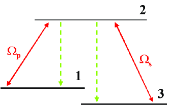
Figure 1: (Color online). States $\left|1\right\rangle$ and $\left|3\right\rangle$ are coherently coupled to level $\left|2\right\rangle$ (red bold lines). The state $\left|2\right\rangle$ is coupled to the other two states by a dipolar system-environment interaction (green dashed lines).

The system interacts with a bosonic bath. The free bath is described by

$$H_{B}=\sum_{k}\omega_{k}\,b_{k}^{\dagger}b_{k}\,,$$ (18)

while the system-bath interaction Hamiltonian is

$$H_{int} = \sum_{k}g_{k}^{(12)}\left(\left|1\right\rangle\left\langle 2\right|+\left|2\right\rangle\left\langle 1\right|\right)(b_{k}+b_{k}^{\dagger})$$ (19)

$$+ \sum_{k}g_{k}^{(32)}\left(\left|3\right\rangle\left\langle 2\right|+\left|2\right\rangle\left\langle 3\right|\right)(b_{k}+b_{k}^{\dagger})\,.$$

In the rotating frame associated with the transformation $T(t)=e^{i\omega_{1}t}\left|1\right\rangle\left\langle 1\right|+e^{i(\omega_{2}-\Delta)t}\left|2\right\rangle\left\langle 2\right|+e^{i\omega_{3}t}\left|3\right\rangle\left\langle 3\right|$, the total Hamiltonian:

$$H=H_{s}(t)+H_{B}+H_{I}(t)\,,$$ (20)

with

$$H_{s}(t)=\left[\begin{array}[]{ccc}0&\Omega_{p}(t)&0\\ \Omega_{p}(t)&\Delta&\Omega_{s}(t)\\ 0&\Omega_{s}(t)&0\\ \end{array}\right]\,,$$ (21)

and

$$H_{I}(t) = \sum_{k}g_{k}^{(12)}\left(e^{i(\omega_{1}-\omega_{2}+\Delta)\,t}\,\left|1\right\rangle\left\langle 2\right|\right.$$ (22)

$$+ \left.e^{-i(\omega_{1}-\omega_{2}+\Delta)\,t}\,\left|2\right\rangle\left\langle 1\right|\right)(b_{k}+b_{k}^{\dagger})$$

$$+ \sum_{k}g_{k}^{(32)}\left(e^{i(\omega_{3}-\omega_{2}+\Delta)\,t}\,\left|3\right\rangle\left\langle 2\right|\right.$$

$$+ \left.e^{-i(\omega_{3}-\omega_{2}+\Delta)\,t}\,\left|2\right\rangle\left\langle 3\right|\right)(b_{k}+b_{k}^{\dagger})\,.$$

The eigenstates and eigenvalues of $H_{s}(t)$ are:

$$\omega_{+}=\Omega_{0}\cot\varphi,\,\,\,\,\omega_{0}=0,\,\,\,\,\omega_{-}=-\Omega_{0}\tan\varphi,$$ (23a)

$$\left|+\right\rangle =\sin\varphi\sin\theta\left|1\right\rangle+\cos\varphi\left|2\right\rangle+\sin\varphi\cos\theta\left|3\right\rangle\,,$$ (23b)

$$\left|0\right\rangle =\cos\theta\left|1\right\rangle-\sin\theta\left|3\right\rangle\,,$$ (23c)

$$\left|-\right\rangle =\cos\varphi\sin\theta\left|1\right\rangle-\sin\varphi\left|2\right\rangle+\cos\varphi\cos\theta\left|3\right\rangle\,,$$ (23d)

where

$$\tan\theta(t) =\frac{\Omega_{p}(t)}{\Omega_{s}(t)}\,,$$ (24a)

$$\tan{2\varphi(t)} =\frac{2\Omega(t)}{\Delta(t)}\,,$$ (24b)

$$\Omega(t) =\sqrt{\Omega_{p}(t)^{2}+\Omega_{s}(t)^{2}}\,.$$ (24c)

It is well known ref:STIRAP_reviews that, for the intuitive sequence of pulses, in which the probe pulse $\Omega_{p}(t)$ precedes the Stokes pulse $\Omega_{s}(t)$, one has $\left|-\right\rangle=\left|1\right\rangle$ for $t\rightarrow-\infty$ and $\left|-\right\rangle=\left|3\right\rangle$ for $t\rightarrow\infty$. Therefore, if all the pulses vary adiabatically, the population of the state $\left|1\right\rangle$ can be transferred to the state $\left|3\right\rangle$: this process is called b-STIRAP. On the other hand, if $\Omega_{s}(t)$ precedes $\Omega_{p}(t)$, one has $\left|0\right\rangle=\left|1\right\rangle$ for $t\rightarrow-\infty$ and $\left|0\right\rangle=\left|3\right\rangle$ for $t\rightarrow\infty$: in this counterintuitive sequence the population from $\left|1\right\rangle$ to $\left|3\right\rangle$ is adiabatically transferred through the state $\left|0\right\rangle$ and the process is called STIRAP.

III.2 Master Equation

Since in the rotating frame we have a slowly-varying system Hamiltonian and a time-dependent system-environment interaction term, we can use the general formalism presented before in order to derive the master equation that describes the dynamics of our system. We obtain the following master equation (for details see appendix A):

$$\dot{\rho} = -i[H_{s},\rho]+\,\left[\gamma_{aa}^{++}(\omega_{+0})\cos^{2}\theta\cos^{2}\varphi+\gamma_{bb}^{++}(\omega_{+0})\sin^{2}\theta\cos^{2}\varphi\right]\left(\left|0\right\rangle\left\langle+\right|\rho\left|+\right\rangle\left\langle 0\right|-\frac{1}{2}\left\{\left|+\right\rangle\left\langle+\right|,\rho\right\}\right)$$ (25)

$$+ \,\left[\gamma_{aa}^{--}(\omega_{0-})\cos^{2}\theta\sin^{2}\varphi+\gamma_{bb}^{--}(\omega_{0-})\sin^{2}\theta\sin^{2}\varphi\right]\left(\left|-\right\rangle\left\langle 0\right|\rho\left|0\right\rangle\left\langle-\right|-\frac{1}{2}\left\{\left|0\right\rangle\left\langle 0\right|,\rho\right\}\right)$$

$$+ \,\left[\gamma_{aa}^{++}(\omega_{+-})\sin^{2}\theta\cos^{4}\varphi+\gamma_{aa}^{--}(\omega_{+-})\sin^{2}\theta\sin^{4}\varphi+\gamma_{bb}^{++}(\omega_{+-})\cos^{2}\theta\cos^{4}\varphi+\gamma_{bb}^{--}(\omega_{+-})\cos^{2}\theta\sin^{4}\varphi\right]$$

$$\times\left(\left|-\right\rangle\left\langle+\right|\rho\left|+\right\rangle\left\langle-\right|-\frac{1}{2}\left\{\left|+\right\rangle\left\langle+\right|,\rho\right\}\right)$$

$$+ \,\left[\left(\gamma_{aa}^{++}(0)+\gamma_{aa}^{--}(0)\right)\sin^{2}\theta\sin^{2}\varphi\cos^{2}\varphi+\left(\gamma_{bb}^{++}(0)+\gamma_{bb}^{--}(0)\right)\cos^{2}\theta\sin^{2}\varphi\cos^{2}\varphi\right]$$

$$\times\left[\left(\left|+\right\rangle\left\langle+\right|-\left|-\right\rangle\left\langle-\right|\right)\rho\left(\left|+\right\rangle\left\langle+\right|-\left|-\right\rangle\left\langle-\right|\right)-\frac{1}{2}\left\{\left|+\right\rangle\left\langle+\right|+\left|-\right\rangle\left\langle-\right|,\rho\right\}\right]$$

$$+ \,\left[\gamma_{aa}^{--}(\omega_{0+})\cos^{2}\theta\cos^{2}\varphi+\gamma_{bb}^{--}(\omega_{0+})\sin^{2}\theta\cos^{2}\varphi\right]\left(\left|+\right\rangle\left\langle 0\right|\rho\left|0\right\rangle\left\langle+\right|-\frac{1}{2}\left\{\left|0\right\rangle\left\langle 0\right|,\rho\right\}\right)$$

$$+ \,\left[\gamma_{aa}^{++}(\omega_{-0})\cos^{2}\theta\sin^{2}\varphi+\gamma_{bb}^{++}(\omega_{-0})\sin^{2}\theta\sin^{2}\varphi\right]\left(\left|0\right\rangle\left\langle-\right|\rho\left|-\right\rangle\left\langle 0\right|-\frac{1}{2}\left\{\left|-\right\rangle\left\langle-\right|,\rho\right\}\right)$$

$$+ \,\left[\gamma_{aa}^{--}(\omega_{-+})\sin^{2}\theta\cos^{4}\varphi+\gamma_{aa}^{++}(\omega_{-+})\sin^{2}\theta\sin^{4}\varphi+\gamma_{bb}^{--}(\omega_{-+})\cos^{2}\theta\cos^{4}\varphi+\gamma_{bb}^{++}(\omega_{-+})\cos^{2}\theta\sin^{4}\varphi\right]$$

$$\times\left(\left|+\right\rangle\left\langle-\right|\rho\left|-\right\rangle\left\langle+\right|-\frac{1}{2}\left\{\left|-\right\rangle\left\langle-\right|,\rho\right\}\right)\,,$$

where $\omega_{nm}=\omega_{n}-\omega_{m}$.

From (13) and (14) one gets that the decay rates are given by a spectral density $J_{j}(\omega)$ multiplied by a factor depending on the photon population $N(\omega)$ of the bath modes at the relevant frequency corrected with $\pm\omega_{a}$ or $\pm\omega_{b}$ depending on the case, i.e.:

$$\!\!\left\{\begin{array}[]{ll}\gamma_{jj}^{++}(\omega)=J_{j}(\omega-\omega_{j})(1+N(\omega-\omega_{j}))&\omega-\omega_{j}>0\,,\\ \gamma_{jj}^{--}(\omega)=J_{j}(\omega+\omega_{j})(1+N(\omega+\omega_{j}))&\omega+\omega_{j}>0\,,\\ \gamma_{jj}^{++}(\omega)=J_{j}(|\omega-\omega_{j}|)\,N(|\omega-\omega_{j}|)&\omega-\omega_{j}<0\,,\\ \gamma_{jj}^{--}(\omega)=J_{j}(|\omega+\omega_{j}|)\,N(|\omega+\omega_{j}|)&\omega+\omega_{j}<0\,,\end{array}\right.$$ (30)

with $j=a,b$ and

$$\omega_{a}=\omega_{1}-\omega_{2}+\Delta\,,$$ (32a)

$$\omega_{b}=\omega_{3}-\omega_{2}+\Delta\,.$$ (32b)

The zero temperature spectral density $J_{j}(\omega)$ for general bosonic reservoir is given by ref:Gardiner ; ref:Petru :

$$J_{j}(\omega)=d(\omega)\,\left|g_{j}(\omega)\right|^{2}$$ (33)

where $g_{a}(\omega)$ ($g_{b}(\omega)$) is the system-reservoir coupling constant $g_{k}^{(12)}$ ($g_{k}^{(32)}$) in the continuum limit, and $d(\omega)$ is the reservoir density of states at frequency $\omega$.

It is important to note that, under the hypothesis that $\omega_{j}\gg\omega$ for any Bohr frequency $\omega$ between the dressed states in the rotating frame (which is the usual case since $\omega_{j}$ are optical frequencies associated with the atomic transitions while $\omega$’s are of the order of magnitude of the coupling terms $\Omega$’s), and taking into account that the frequencies in (32a) are negative, the only condition satisfied are $\omega-\omega_{j}>0$ and $\omega+\omega_{j}<0$. Therefore, in (30), only the rates of the first and fourth classes are possible. Moreover, at zero temperature only the rates of the first class survive, since the number of photons in the reservoir is zero. In such a case the master equation becomes:

$$\dot{\rho} = -i[H_{s},\rho]+\,\left[\gamma_{aa}^{++}(\omega_{+0})\cos^{2}\theta\cos^{2}\varphi+\gamma_{bb}^{++}(\omega_{+0})\sin^{2}\theta\cos^{2}\varphi\right]\left(\left|0\right\rangle\left\langle+\right|\rho\left|+\right\rangle\left\langle 0\right|-\frac{1}{2}\left\{\left|+\right\rangle\left\langle+\right|,\rho\right\}\right)$$ (34)

$$+ \,\left[\gamma_{aa}^{++}(\omega_{-0})\cos^{2}\theta\sin^{2}\varphi+\gamma_{bb}^{++}(\omega_{-0})\sin^{2}\theta\sin^{2}\varphi\right]\left(\left|0\right\rangle\left\langle-\right|\rho\left|-\right\rangle\left\langle 0\right|-\frac{1}{2}\left\{\left|-\right\rangle\left\langle-\right|,\rho\right\}\right)$$

$$+ \,\left[\gamma_{aa}^{++}(\omega_{+-})\sin^{2}\theta\cos^{4}\varphi+\gamma_{bb}^{++}(\omega_{+-})\cos^{2}\theta\cos^{4}\varphi\right]\times\left(\left|-\right\rangle\left\langle+\right|\rho\left|+\right\rangle\left\langle-\right|-\frac{1}{2}\left\{\left|+\right\rangle\left\langle+\right|,\rho\right\}\right)$$

$$+ \,\left[\gamma_{aa}^{++}(\omega_{-+})\sin^{2}\theta\sin^{4}\varphi+\gamma_{bb}^{++}(\omega_{-+})\cos^{2}\theta\sin^{4}\varphi\right]\times\left(\left|+\right\rangle\left\langle-\right|\rho\left|-\right\rangle\left\langle+\right|-\frac{1}{2}\left\{\left|-\right\rangle\left\langle-\right|,\rho\right\}\right)$$

$$+ \,\left[\gamma_{aa}^{++}(0)\sin^{2}\theta\sin^{2}\varphi\cos^{2}\varphi+\gamma_{bb}^{++}(0)\cos^{2}\theta\sin^{2}\varphi\cos^{2}\varphi\right]$$

$$\times\left[\left(\left|+\right\rangle\left\langle+\right|-\left|-\right\rangle\left\langle-\right|\right)\rho\left(\left|+\right\rangle\left\langle+\right|-\left|-\right\rangle\left\langle-\right|\right)-\frac{1}{2}\left\{\left|+\right\rangle\left\langle+\right|+\left|-\right\rangle\left\langle-\right|,\rho\right\}\right]$$

This equation shows that at zero temperature there are the following processes: transitions from $\left|+\right\rangle$ to $\left|-\right\rangle$ and vice versa, transitions from $\left|+\right\rangle$ to $\left|0\right\rangle$ and from $\left|-\right\rangle$ to $\left|0\right\rangle$, and a dephasing process involving levels $\left|+\right\rangle$ and $\left|-\right\rangle$ (see figure 2). This suggests the idea that the damping can help to transfer population to level $\left|0\right\rangle$, so that the efficiency of the counterintuitive sequence should be positively affected by the dissipation.

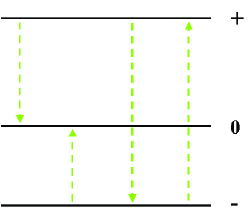
Figure 2: (Color online). Scheme of the decays for the dressed states. There are transitions from $\left|+\right\rangle$ to $\left|-\right\rangle$ and vice versa. Both $\left|+\right\rangle$ and $\left|-\right\rangle$ decay toward $\left|0\right\rangle$. The dephasing between the states $\left|+\right\rangle$ and $\left|-\right\rangle$ is not represented.

IV Analysis of the Efficiency at Zero Temperature

In this section we analyze the efficiency of both STIRAP and b-STIRAP processes, by numerically studying the post-pulse population of the target state $\left|3\right\rangle$ and compare the prediction of our model with the predictions of a phenomenological model introduced in ref. STIRAP spontaneous emission .

We consider Gaussian laser pulses:

$$\Omega_{1} = \frac{\Omega_{0}}{2}\,e^{-(t-\tau/2)^{2}/T^{2}}\,,$$ (35a)

$$\Omega_{2} = \frac{\Omega_{0}}{2}\,e^{-(t+\tau/2)^{2}/T^{2}}\,,$$ (35b)

taking into account that we have the so called intuitive sequence (which corresponds to b-STIRAP) when $\Omega_{p}=\Omega_{2}$ and $\Omega_{s}=\Omega_{1}$, while we get the counterintuitive sequence (which corresponds to STIRAP) when $\Omega_{p}=\Omega_{1}$ and $\Omega_{s}=\Omega_{2}$.

The phenomenological model which we will compare with our microscopic model corresponds to the following master equation:

$$\dot{\rho}=-i[H,\rho]-\frac{1}{2}D\,,$$ (36)

with

$$D=\left(\begin{array}[]{ccc}-2\Gamma_{1}\rho_{22}&(\Gamma_{1}+\Gamma_{3})\rho_{12}&0\\ (\Gamma_{1}+\Gamma_{3})\rho_{21}&2(\Gamma_{1}+\Gamma_{3})\rho_{22}&(\Gamma_{1}+\Gamma_{3})\rho_{23}\\ 0&(\Gamma_{1}+\Gamma_{3})\rho_{32}&-2\Gamma_{3}\rho_{22}\end{array}\right)\,,$$ (40)

which describes spontaneous emission from level $2$ to levels $1$ and $3$ with rates $\Gamma_{1}$ and $\Gamma_{3}$, respectively. Such a master equation is related to the bare states and then turns out to be time-independent.

Concerning the microscopic model, we assume flat spectrum for both the transitions $2\rightarrow 1$, corresponding to $J_{a}(\omega)$, and $2\rightarrow 3$, corresponding to $J_{b}(\omega)$. In particular we will assume $J_{a}(\omega)\equiv\Gamma$ and $J_{b}(\omega)\equiv\alpha\Gamma$. This may come, for instance, from the assumption that the dipole moments between the states $\left|1\right\rangle$ and $\left|2\right\rangle$ and between the states $\left|3\right\rangle$ and $\left|2\right\rangle$ are proportional, so that $g_{k}^{(12)}=\alpha g_{k}^{(32)}$ for any $k$ in eq. (19).

IV.1 The counterintuitive sequence

We first analyze the counterintuitive sequence, where the population is carried by the dark state $\left|0\right\rangle$.

Figure 3 shows the comparison between the microscopic and the phenomenological models, with $\alpha=1$ and $\Gamma_{1}=\Gamma_{2}=\Gamma$. It is evident that the microscopic model predicts a very high efficiency (essentially one) for a wider range of $\Gamma$. This can be explained on the basis of the decay scheme in fig. 2: all the decay processes describe either jumps toward $\left|0\right\rangle$ or toward states which in turn decay toward $\left|0\right\rangle$, so that the dark state is robust against zero temperature dissipation.

The robustness of the counterintuitive scheme is not related to the special choice $\alpha=1$. Indeed, figure 4 shows the dependence of the post-pulse population of state $\left|3\right\rangle$ on both $\Gamma$ and the parameter $\alpha$ which characterizes the difference in the intensities of the dipolar coupling constant involving different couples of levels. It is quite evident that the efficiency of the scheme is not affected by a discrepancy in the decay rates.

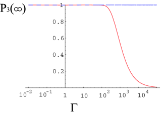
Figure 3: (Color online). Counterintuitive sequence. Final population vs $\Gamma$ (in units of $T^{-1}$ and in logarithmic scale) according to microscopic (dashed blue line) and phenomenological (solid red line) model. The relevant parameters are $\Omega_{0}=25\,T^{-1}$, $\tau=1.5\,T^{-1}$, $T\,\Delta=1$, $\alpha=1$.

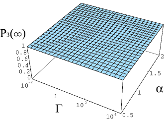
Figure 4: (Color online). Counterintuitive sequence. Final population vs both $\Gamma$ (in units of $T^{-1}$ and in logarithmic scale) and $\alpha$ according to the microscopic model. The relevant parameters are $\Omega_{0}=25\,T^{-1}$, $\tau=1.5\,T^{-1}$, $T\,\Delta=1$.

IV.2 The intuitive sequence

Concerning the b-STIRAP process (i.e. in the intuitive sequence), we find that the two models predict very similar results. In particular, fig. 5 shows the perfect coincidence of the predictions of the two models in the case $\alpha=1$ and $\Gamma_{1}=\Gamma_{2}=\Gamma$. Moreover, from this figure one can see that (for both models) the efficiency is very sensitive to the presence of decays, so that it almost drops to zero at $\Gamma\,T=1$. The reason of the fragility of the efficiency in this scheme is that, while all the populations are guided by the decay towards the state $\left|0\right\rangle$, population transfer is instead carried on by the state $\left|-\right\rangle$.

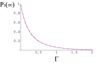
Figure 5: (Color online). Intuitive sequence. Final population vs $\Gamma$ (in units of $T^{-1}$) according to microscopic (dashed blue line) and phenomenological (solid red line) model. The relevant parameters are $\Omega_{0}=25\,T^{-1}$, $\tau=1.5\,T^{-1}$, $T\,\Delta=1$, $\alpha=1$. The two curves are essentially coincident.

It is worth noting that the result of the comparison is qualitatively quite similar to the result of the comparison we made in connection to the scheme with external decay ref:Scala2010 . Indeed, in both cases the predictions from the microscopic and the phenomenological models are almost coincident for the intuitive sequence, while for the counterintuitive sequence we find that the microscopic model predicts a higher efficiency. Nevertheless, we stress here the fact that the enhancement of efficiency in STIRAP in the strong damping limit is due to very different mechanisms in the two cases of external and internal decay. In fact, while for external decay a very strong damping is responsible for a dynamical decoupling of the dark state, which then is protected against losses, in the case of internal decay the dissipation is instead responsible for transitions toward the state that carries the population, therefore protecting the process of population transfer.

V Analysis of the Efficiency at Nonzero Temperature

In this section we consider the effects of nonzero temperature. Looking at (30), we see that the $N(\omega)$’s are evaluated at very close frequencies, which are essentially $\omega\approx\omega_{21}\approx\omega_{23}$. For this reason, we described temperature by a single number $N$ which is the number of photons in the reservoir modes of frequencies close to the bare atomic transitions.

We have seen that at zero temperature, for increasing $\Gamma$ (and even for quite small values of the decay constant) the efficiency falls down to zero when the intuitive sequence is applied. When temperature is non-vanishing all the transitions included in (25) but not present in (34) must be considered. In particular, transitions from $\left|0\right\rangle$ to $\left|-\right\rangle$ should increase the efficiency of the b-STIRAP process, since in this scheme the population is transferred through the state $\left|-\right\rangle$. On the other hand, in the counterintuitive sequence we should get a lower transfer efficiency, since thermal terms are responsible for loss of population from state $\left|0\right\rangle$ during the STIRAP process.

Figure 6a shows the dependence of the post-pulse population of the state $\left|3\right\rangle$ on $\Gamma$ and temperature (through the number of photons $N$ in the relevant reservoir modes), for the intuitive sequence. It is well visible that the efficiency, which goes to zero for large $\Gamma$ in the zero temperature regime, reaches nonzero values for non vanishing temperature. Such efficiency reaches a maximum value for intermediate values of temperature. As an example, figure 6b shows the temperature dependence (in a wider range) of the efficiency for $\Gamma=1$: in this case the optimal point is reached at $N\simeq 10$.

Figure 7 shows the post-pulse population of the state $\left|3\right\rangle$ on $\Gamma$ and temperature for the counterintuitive sequence. In this case it is well visible that the temperature negatively affects the efficiency of the population transfer. Indeed, even a very small amount of thermal photons is responsible for a significant diminishing of the post-pulse population, which instead approaches unity at rigorously zero temperature.

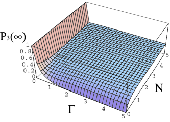
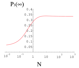
Figure 6: (Color online). Intuitive sequence. (a) Final population vs $\Gamma$ (in units of $T^{-1}$) and the number of photons $N$. (b) Final population vs the number of photons $N$ (in logarithmic scale) , for $\Gamma=1$. In both cases, the relevant parameters are $\Omega_{0}=25\,T^{-1}$, $\tau=1.5\,T^{-1}$, $T\,\Delta=1$, $\alpha=1$.

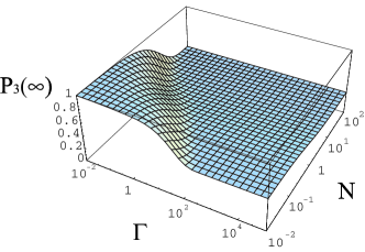
Figure 7: (Color online). Counterintuitive sequence. Final population vs $\Gamma$ (in units of $T^{-1}$ and in logarithmic scale) and the number of photons $N$ (in logarithmic scale). The relevant parameters are $\Omega_{0}=25\,T^{-1}$, $\tau=1.5\,T^{-1}$, $T\,\Delta=1$, $\alpha=1$.

VI Discussion and Conclusive Remarks

In this paper we have analyzed the effects on a STIRAP scheme of the losses of the auxiliary level towards the two metastable states, examined by means of the numerical resolution of a master equation which has been microscopically derived. It is worth noting that, in order to remove the rapid oscillations in the system Hamiltonian, we are forced to describe the system in a rotating frame, where the system-bath interaction term turns out to be time-dependent. Therefore, when deriving the master equation we have to deal both with a slowly varying system Hamiltonian, which can be treated following the general theory by Davies and Spohn, and a rapidly oscillating system-environment interaction term. This last point makes the final master equation different from what one usually gets. Indeed the zero temperature transitions are not guiding the system towards the dressed (rotating) ground state $\left|-\right\rangle$, but instead towards the state $\left|0\right\rangle$. In this sense, the oscillating terms in the system-environment interaction act like a pumping which makes the counterintuitive sequence much more robust than the intuitive sequence.

The inclusion of the nonzero temperature terms in the master equation partially modifies these conclusions. In fact, thermal photons switch on different transitions, which make the post-pulse population of state $\left|-\right\rangle$ different from zero. As a consequence the efficiency of the counterintuitive sequence is reduced, while on the other hand the efficiency of the intuitive sequence increases. However, such an increasing is not high enough to make the intuitive sequence preferable to the counterintuitive one.

Though the analysis of this STIRAP scheme (with the same decay channels), performed in previous papers by means of phenomenological dissipative terms, has shown a high robustness of the counterintuitive sequence with respect to losses, our analysis shows that the scheme at zero temperature is much more robust for very high decay rates. This is due to the fact that, as already pointed out, the zero temperature decay channels force the system to the state $\left|0\right\rangle$, which is the population carrier in this sequence.

Appendix A Derivation of the Master Equation

In this appendix we give some more details about the derivation of the master equation in our model. In our case we consider:

$$A_{a}^{+} = \left|1\right\rangle\left\langle 2\right|\,,$$ (42a)

$$A_{a}^{-} = \left|2\right\rangle\left\langle 1\right|\,,$$ (42b)

$$A_{b}^{+} = \left|3\right\rangle\left\langle 2\right|\,,$$ (42c)

$$A_{b}^{-} = \left|2\right\rangle\left\langle 3\right|\,,$$ (42d)

$$B_{a}=\sum_{k}g_{k}^{(12)}(b_{k}+b_{k}^{\dagger})\,,$$ (43a)

$$B_{b}=\sum_{k}g_{k}^{(32)}(b_{k}+b_{k}^{\dagger})\,,$$ (43b)

from which we obtain the following jump operators:

$$\begin{array}[]{ll}A_{a}^{+}(\omega_{+0})=\cos\theta\cos\varphi\left|0\right\rangle\left\langle+\right|\,,&A_{a}^{-}(\omega_{+0})=0\,,\\ A_{b}^{+}(\omega_{+0})=-\sin\theta\cos\varphi\left|0\right\rangle\left\langle+\right|\,,&A_{b}^{-}(\omega_{+0})=0\,,\\ A_{a}^{+}(\omega_{0-})=0\,,&A_{a}^{-}(\omega_{0-})=-\cos\theta\sin\varphi\left|-\right\rangle\left\langle 0\right|\,,\\ A_{b}^{+}(\omega_{0-})=0\,,&A_{b}^{-}(\omega_{0-})=\sin\theta\sin\varphi\left|-\right\rangle\left\langle 0\right|\,,\\ A_{a}^{+}(\omega_{+-})=\sin\theta\cos^{2}\varphi\left|-\right\rangle\left\langle+\right|\,,&A_{a}^{-}(\omega_{+-})=-\sin\theta\sin^{2}\varphi\left|-\right\rangle\left\langle+\right|\,,\\ A_{b}^{+}(\omega_{+-})=\cos\theta\cos^{2}\varphi\left|-\right\rangle\left\langle+\right|\,,&A_{b}^{-}(\omega_{+-})=-\cos\theta\sin^{2}\varphi\left|-\right\rangle\left\langle+\right|\,,\\ \end{array}$$ (50)

$$\,\,A_{a}^{+}(0)=A_{a}^{-}(0)=\sin\theta\sin\varphi\cos\varphi\left(\left|+\right\rangle\left\langle+\right|-\left|-\right\rangle\left\langle-\right|\right)\,,$$

$$\,\,A_{b}^{+}(0)=A_{b}^{-}(0)=\cos\theta\sin\varphi\cos\varphi\left(\left|+\right\rangle\left\langle+\right|-\left|-\right\rangle\left\langle-\right|\right)\,.$$ (51)

Putting all the jump operators inside the Lindblad form in (16), we get the master equation in (25).

References

- (1) A. Messiah, Quantum Mechanics (Dover publications, 1999)
- (2) J. I. Cirac, R. Blatt, and P. Zoller, Phys. Rev. A 49, R3174 (1994)
- (3) D. Leibfried, B. DeMarco, V. Meyer, D. Lucas, M. Barrett, J. Britton, W. M. Itano, B. Jelenkovic, C. Langer, T. Rosenband, and D. J. Wineland, Nature 422, 412-415 (2003).
- (4) M. V. Berry, Proc. R. Soc. Lond. A, 392, 45-57 (1984); M. V. Berry, J. Mod. Opt., 34, 1401-1407 (1987); J. Samuel and R. Bhandari, Phys. Rev. Lett. 60, 2339 (1987).
- (5) K.-P. Marzlin and B. C. Sanders, Phys. Rev. Lett. 93, 160408 (2004).
- (6) D. Comparat, Phys. Rev. A 80, 012106 (2009).
- (7) U. Gaubatz, P. Rudecki, S. Schiemann, K. Bergmann, J. Chem. Phys. 92, 5363 (1990).
- (8) S. Schiemann, A. Kuhn, S. Steuerwald, K. Bergmann, Phys. Rev. Lett. 71, 3637 (1993).
- (9) For reviews see: N. V. Vitanov, M. Fleischhauer, B. W. Shore and K. Bergmann, Adv. At. Mol. Opt. Phys. 46, 55 (2001); N. V. Vitanov, T. Halfmann, B. W. Shore and K. Bergmann, Ann. Rev. Phys. Chem. 52, 763 (2001); K. Bergmann, H. Theuer, and B. W. Shore, Rev. Mod. Phys. 70, 1003 (1998); P. Král, I. Thanopoulos, and M. Shapiro, Rev. Mod. Phys. 79, 53 (2007).
- (10) Q. Shi and E. Geva, J. Chem. Phys. 119, 11773 (2003); P. A. Ivanov, N. V. Vitanov, and K. Bergmann, Phys. Rev. A 70, 063409 (2004).
- (11) N. V. Vitanov and S. Stenholm, Phys. Rev. A 56, 1463 (1997).
- (12) P. A. Ivanov, N. V. Vitanov, and K. Bergmann, Phys. Rev. A 72, 053412 (2005).
- (13) M. Scala, B. Militello, A. Messina, and N. Vitanov, Phys. Rev. A 81, 053847 (2010).
- (14) P. Pillet, C. Valentin, R.-L. Yuan, and J. Yu, Phys. Rev. A 48, 845 (1993); C. Valentin, J. Yu, and P. Pillet, J. Physique II France 4, 1925 (1994).
- (15) L.S. Goldner, C. Gerz, R.J.C. Spreeuw, S.L. Rolston, C.I. Westbrook, W.D. Phillips, P. Marte, and P. Zoller, Phys. Rev. Lett. 72, 997 (1994).
- (16) D. S. Weiss, B. C. Young, and S. Chu, Appl. Phys. B 59, 217 (1994); M. Weitz, B. C. Young, and S. Chu, Phys. Rev. A 50, 2438 (1994).
- (17) T. Halfmann and K. Bergmann, J. Chem. Phys. 104, 7068 (1996).
- (18) H. Theuer and K. Bergmann, Eur. Phys. J. D 2, 279 (1998).
- (19) E. B. Davies and H. Spohn, J. Stat. Phys. 19, 511 (1978).
- (20) G. Florio, P. Facchi, R. Fazio, V. Giovannetti, and S.Pascazio, Phys. Rev. A 73, 022327 (2006).
- (21) C. W. Gardiner and P. Zoller, Quantum Noise (Springer-Verlag, Berlin, 2000).
- (22) H.-P. Breuer and F. Petruccione, The Theory of Open Quantum Systems (Oxford University Press, Oxford, 2002).