Transport properties of a spin-$\frac{1}{2}$ Heisenberg chain with an embedded spin-$S$ impurity

Abstract

The finite temperature transport properties of a spin-$\frac{1}{2}$ anisotropic Heisenberg chain with an embedded spin-$S$ impurity are studied. Using primarily numerical diagonalization techniques, we study the dependence of the dynamical spin and thermal conductivities on the lattice size, the magnitude of the impurity spin, the host-impurity coupling, the easy axis anisotropy, as well as the dependence on temperature. Particularly for the temperature dependence, we discuss the screening of the impurity by the chain eventually leading to the cutting or healing of the host chain. Numerical results are supported by analytical arguments obtained in the strong host-impurity coupling regime.

I Introduction

The unconventional thermal transport properties of low dimensional quantum magnets have drawn the attention of the condensed matter society.Zotos and Prelovšek (2004); Alvarez and Gros (2002a); Heidrich-Meisner et al. (2002); Orignac et al. (2003); Louis and Gros (2003); Saito (2003); Heidrich-Meisner et al. (2005); Shimshoni et al. (2003); Rozhkov and Chernyshev (2005); Jung et al. (2006); Karahalios et al. (2009); Sologubenko et al. (2007); Hess (2007); Otter et al. (2009); Saito and Miyashita (2002) In particular, the transport properties of spin chain materials are described by the one-dimensional (1D) spin-$\frac{1}{2}$ Heisenberg model, where the large exchange coupling along the chainEggert et al. (1994); Eggert (1996); Motoyama et al. (1996) accounts for an extraordinary high and anisotropic thermal conductivity.Sologubenko et al. (2001) Actually, the pure anisotropic Heisenberg model (AHM) was shown to exhibit ballistic thermal transport at any temperature $T$, attributed to its integrability.Zotos et al. (1997); Klümper and Sakai (2002); Sakai and Klümper (2003) In accord with the theoretical predictions, evidence of ballistic thermal transport in real materials has been consolidated lately using samples of very high purity.Hlubek et al. (2010) However, defects may have a dramatic effect on the transport properties of these systems due to the reduced dimensionality.

In this work, we try to shed light on the effect of a single, spin-$S$ magnetic impurity, on the transport properties of a spin-$\frac{1}{2}$ Heisenberg chain. We address the behavior of the system on various problem parameters at high and intermediate $T$, while we support our numerical results with analytical arguments. It is well known that magnetic impurities get screened by the chain at low $T$ forming with their neighbors an effective impurity of different spin.Eggert and Affleck (1992); Eggert et al. (2001); Mahajan and Venkataramani (2001) Notwithstanding, as we show in this work, conspicuous excitations, which cannot be described by the effective impurity picture, survive at low $T$; this holds for a single impurity in a finite system or plausibly for a finite concentration of impurities in the thermodynamic limit. Furthermore, the screening of the impurity triggers Kondo-type, many body, phenomena below a crossover temperature, and the chain becomes perfectly (insulating)transmitting at $T=0$ for (anti)ferromagnetic easy axis anisotropy $\Delta$.Furusaki and Hikihara (1998); Metavitsiadis et al. (2010) This is an analog of the behavior of a Luttinger liquid in the presence of a non-magnetic impurity where the chain is (cut)healed for (repulsive)attractive interactions.Kane and Fisher (1992) We seek evidence of the cutting-healing behavior of the chain using the thermal conductivity as a probe, which is ideal for this purpose since the only energy current relaxation mechanism is induced by the impurity.

From the above it is obvious that the role of the thermal conductivity in these systems is exceptional and twofold. Not only is the thermal conductivity a very useful theoretical tool but it is of high experimental and technological interests as well. Thus, our results could serve as qualitative guidelines for forthcoming thermal conductivity measurements in doped cuprates, e.g., $\mathrm{Ni}$ doping in the renowned $\mathrm{SrCuO}_{2}$ and $\mathrm{Sr}_{2}\mathrm{CuO}_{3}$ cuprates. Furthermore, magnetic impurities in highly heat conducting materials could function as potential switching mechanisms enabling tunable heat transport and the emergence of numerous technological applications. Therefore, it is vital to understand the fundamental properties of a prototype model in the presence of magnetic impurities before trying to exploit the transport properties of these truly unique systems.

II Model

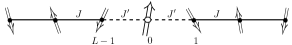
Figure 1: Spin-$S$ impurity embedded in a spin-$\frac{1}{2}$ chain.

In a previous work,Metavitsiadis et al. (2010) the thermal transport properties of a spin-$\frac{1}{2}$ Heisenberg chain was studied in the presence of a spin-$S$ magnetic impurity located out of the chain. In addition, a uniform chain with two consecutive weak links was discussed, which can be considered as a special case of a spin-$\frac{1}{2}$ impurity embedded in the chain. In the present work, we deal with the generic case of a spin-$S$ magnetic impurity embedded in the chain, Fig. 1. Many of the conclusions and the basic ideas reached in Ref.Metavitsiadis et al. (2010) can be applied in the present work, as well, due to the single impurity character of the problem. However, significant differences in the physical results arise due to the different geometries of the problems. A brief discussion and comparison between the two models is given at the end of the manuscript.

The Hamiltonian of an AHM on a ring of $L$ sites, where a spin-$\frac{1}{2}$ operator, say the $\mathbf{s}_{0}$, is substituted by another one of different spin, say $\mathbf{S}$, is given by

$$H=\sum_{l=1}^{L-2}h_{l}+J^{\prime}~{}\big{(}\mathbf{s}_{1}+\mathbf{s}_{L-1}\big{)}\cdot\tilde{\mathbf{S}}\>,\quad\big{(}h_{l}=J\mathbf{s}_{l}\cdot\tilde{\mathbf{s}}_{l+1}\big{)}\>,$$ (1)

see Fig. 1 as well. In Eq. (1), $J$ is the antiferromagnetic exchange coupling—with energy units—between spin-$\frac{1}{2}$ operators, $J^{\prime}$ is the host-impurity coupling, while the tilded operators $\tilde{\mathbf{s}}$, $\tilde{\mathbf{S}}$ denote the vector operators $(s^{x},s^{y},\Delta s^{z})$, $(S^{x},S^{y},\Delta S^{z})$, respectively. In addition, we work in a system of units where the lattice constant $a$, and the Planck and Boltzmann constants are $a,\hslash,k_{B}=1$; yet numerical results are presented for $J=1$.

The spin $\jmath^{s}$, energy $\jmath^{\epsilon}$ current operators are determined by the continuity equation $\partial_{t}{\hat{O}}_{l}+\nabla\mathcal{J}_{l}=0$. Taking $\hat{O}_{l}$ to be the local spin, energy operators and $\mathcal{J}_{l}$ to be the local spin, energy current operators respectively, we arrive at

$$\jmath^{s}=\sum_{l=1}^{L-2}J\big{(}\mathbf{s}_{l}\times\mathbf{s}_{l+1}\big{)}\cdot\hat{e}_{z}+J^{\prime}\big{[}\big{(}\mathbf{s}_{L-1}-\mathbf{s}_{1}\big{)}\times\mathbf{S}\big{]}\cdot\hat{e}_{z}\>,$$ (2)

where $\hat{e}_{z}$ is the unit vector along the $z$-axis, and

$$\jmath^{\epsilon} = \sum_{l=2}^{L-2}J^{2}\mathbf{s}_{l}\cdot\big{(}\tilde{\mathbf{s}}_{l+1}\times\tilde{\mathbf{s}}_{l-1}\big{)}+JJ^{\prime}\mathbf{s}_{1}\cdot\big{(}\tilde{\mathbf{s}}_{2}\times\tilde{\mathbf{S}}\big{)}$$ (3)

$$+ JJ^{\prime}\mathbf{s}_{L-1}\cdot\big{(}\tilde{\mathbf{S}}\times\tilde{\mathbf{s}}_{L-2}\big{)}+J^{\prime 2}\mathbf{S}\cdot\big{(}\tilde{\mathbf{s}}_{1}\times\tilde{\mathbf{s}}_{L-1}\big{)}\>.$$

Within linear response theory, the real part of the spin $\sigma^{\prime}$, thermal $\kappa^{\prime}$ conductivities are given byKubo (1957); Luttinger (1964); Shastry (2006)

$$\sigma^{\prime}(\omega)=2\pi D_{S}\delta(\omega)+\sigma(\omega)\>,~{}~{}\kappa^{\prime}(\omega)=2\pi D_{E}\delta(\omega)+\kappa(\omega)\>,$$

where the corresponding spin $D_{S}$, energy $D_{E}$ stiffnesses denote the presence of ballistic transport in the system. The regular components $\sigma$, $\kappa$ of the corresponding spin, thermal conductivities are given by

$$\sigma(\omega)\hskip-2.84544pt = \hskip-2.84544pt\frac{\pi}{L}\frac{1-e^{-\beta\omega}}{\omega}\hskip-4.26773pt\sum_{\begin{subarray}{c}n,m\\ (\epsilon_{n}\neq\epsilon_{m})\end{subarray}}\hskip-4.26773ptp_{n}|\langle n|\jmath^{s}|m\rangle|^{2}\delta(\omega_{mn}-\omega),~{}~{}$$ (4)

$$\kappa(\omega)\hskip-2.84544pt = \hskip-2.84544pt\frac{\pi\beta}{L}\frac{1-e^{-\beta\omega}}{\omega}\hskip-8.5359pt\sum_{\begin{subarray}{c}n,m\\ (\epsilon_{n}\neq\epsilon_{m})\end{subarray}}\hskip-5.69046ptp_{n}|\langle n|\jmath^{\epsilon}|m\rangle|^{2}\delta(\omega_{mn}-\omega),~{}~{}$$ (5)

where $\epsilon_{n}$ are the eigenvalues and $|n\rangle$ are the eigenstates of the Hamiltonian (1), $p_{n}=\exp(-\beta\epsilon_{n})/Tr\exp(-\beta H)$, $\omega_{mn}=\epsilon_{m}-\epsilon_{n}$, and $\beta=1/T$.

While in the pure AHM it is clear that $D_{E}$ is finite for any value of the easy axis anisotropy $\Delta$,Zotos et al. (1997); Klümper and Sakai (2002); Sakai and Klümper (2003) there is an ongoing debate on the behavior of the spin stiffness.Sirker et al. (2009); Heidrich-Meisner et al. (2003); Benz et al. (2005); Steinigeweg and Schnalle (2010); Alvarez and Gros (2002b); Shastry and Sutherland (1990); Zotos and Prelovšek (1996); Peres et al. (1999); Narozhny et al. (1998) Nevertheless, a single impurity renders ballistic transport incoherent and both $D_{S}$, $D_{E}$ vanish.Barišić et al. (2009) Thus, the static component of the transport quantities is given by the resistive dc spin, thermal conductivities obtained by the zero frequency limit of the regular components (4), (5), viz., $\sigma_{dc}=\sigma(\omega\rightarrow 0)$, $\kappa_{dc}=\kappa(\omega\rightarrow 0)$.

To numerically study transport quantities for systems with a Hilbert space dimension up to $\mathcal{D}\sim 10^{4}$, at high temperatures, we employ the exact diagonalization (ED) technique. The $\delta$-peaks at the excitation frequencies are binned in windows $\delta\omega=0.01$ while we introduce an additional broadening $\eta=0.03$ using the well-known Kramers-Kronig relations. For $\mathcal{D}\gtrsim 10^{4}$, we use the microcanonical Lanczos methodLong et al. (2003) (MCLM) at high temperatures and the finite temperature Lanczos methodJaklič and Prelovšek (2000) (FTLM) at finite temperatures; yet we keep the same additional broadening. Lastly, all results are obtained in the $S^{z}_{\text{total}}=0$ subsector.

III Numerical results

III.1 Spin-1 impurity

First, we would like to address the $S=1$ impurity case since this may be the most appealing magnetic impurity doping for experiments. In Fig. 2, we present results for the dc spin $\sigma_{dc}$, thermal $\kappa_{dc}$ conductivities, while in Figs.  3, and 4 we present the dynamical thermal conductivity of the isotropic ($\Delta=1$) Heisenberg chain. A wide range of host-impurity couplings, $J^{\prime}/J=0.4-2.0$, is shown at high temperatures, $\beta\rightarrow 0$, for various lattice sizes, $L=15-21$. Results for $L=15$ are obtained via the ED technique, while results for $L>15$ are obtained by employing the MCLM. In order to eliminate unimportant for this discussion prefactors of the transport quantities, we plot either the normalized thermal conductivity, $\bar{\kappa}(\omega)=\kappa(\omega)/\kappa_{0}$ where the normalization $\kappa_{0}$ is given by $\kappa_{0}=\int\kappa(\omega)d\omega$, or the non-trivial at high temperatures $T\sigma_{dc}$, $T\sigma(\omega)$, $T^{2}\kappa_{dc}$ and $T^{2}\kappa(\omega)$. Finally, for the discussion of the lattice size scaling we plot the scaled thermal conductivity $\kappa(\omega L)/L$.Metavitsiadis et al. (2010); Barišić et al. (2009)

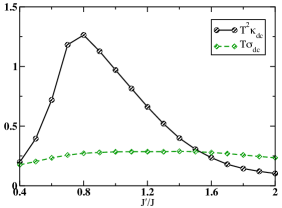
Figure 2: (color online). The dc value of the thermal $T^{2}\kappa_{dc}$, spin $T\sigma_{dc}$ conductivity is shown as a function of the host-impurity coupling $J^{\prime}/J$, obtained via ED for $L=15$, $S=1$, $\Delta=1$, and $\beta\rightarrow 0$.

For a very weak or very strong $J^{\prime}$, a severe reduction of $\kappa_{dc}$ from its maximum value, which occurs at $J^{\prime}=0.8J$, is illustrated in Fig. 2. On the contrary, the behavior of $\sigma_{dc}$ is qualitatively different from the one of $\kappa_{dc}$. Besides the qualitative difference, it is rather impressive that $\sigma_{dc}$ hardly changes in the wide range of $J^{\prime}$ shown in Fig. 2. Although it is reasonable that $\sigma$ will be less sensitive to the effect of the single impurity due to the bulk scattering—$[H,\jmath^{s}]\neq 0$ in the pure model—its rigidity is still surprising.

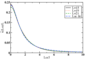
Figure 3: (color online). The frequency dependence of the normalized and scaled thermal conductivity $\bar{\kappa}(\omega L)/L$ is shown for $L=15,19,21$ and $J^{\prime}/J=0.8$; in addition a Lorentzian fit is depicted. Results are obtained for $S=1$, $\Delta=1$, and $\beta\rightarrow 0$. $L=15$ results are obtained via ED and $L>15$ via MCLM.

In Fig. 3, $\bar{\kappa}(\omega L)/L$ is depicted for $J^{\prime}=0.8J$ and a Lorentzian fit as well, signifying the Lorentzian behavior of $\kappa$, $\kappa(\omega)=\kappa_{dc}/[1+(\omega\tau^{\epsilon})^{2}]$ with $\tau^{\epsilon}$ the scattering time. The thermal conductivity retains its Lorentzian shape, approximately, in a range of values of the host-impurity coupling, $J^{\prime}/J\simeq 0.8\pm 0.2$. As previously proposed,Metavitsiadis et al. (2010) a Lorentzian form of $\kappa(\omega)$ is an indication of a weak perturbation, while on the contrary a non-monotonic form implies that the system has flown to the strong perturbation regime. The Lorentzian behavior is retained, with an almost constant $\tau^{\epsilon}$, for temperatures as low as the limiting FTLM temperature for finite size systems $T_{fs}$ below which FTLM results are not reliable;Jaklič and Prelovšek (2000) we estimate $T_{fs}/J\simeq 0.3$. Although $T_{fs}$ is sufficient to reveal the cutting of the chain for strong perturbations,Eggert and Affleck (1992) for weak perturbations a lower $T_{fs}$ is required.Metavitsiadis et al. (2010) To obtain an impression of $T_{fs}$, consider that for systems like the $\mathrm{Sr}_{2}\mathrm{CuO}_{3}$ compound with $J/k_{B}\approx 2500$ K, $T_{fs}\approx 750$ K. However, defects may reduce $J$ of doped samplesMahajan and Venkataramani (2001) bringing $T_{fs}$ closer to room temperature.

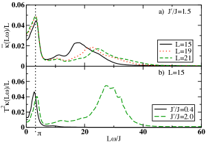
Figure 4: (color online). a) The frequency dependence of the normalized and scaled thermal conductivity $\bar{\kappa}(\omega L)/L$ is shown for $L=15,19,21$ and $J^{\prime}/J=1.5$. b) The frequency dependence of $T^{2}\kappa(\omega L)/L$ is shown for $L=15$ and two host-impurity couplings $J^{\prime}/J=0.4,2.0$. Results are obtained for $S=1$, $\Delta=1$, and $\beta\rightarrow 0$. $L=15$ results are obtained via ED and $L>15$ via MCLM.

For extreme values of the coupling $J^{\prime}$, either strong or weak, $\kappa(\omega)$ exhibits a strongly non-monotonic behavior, Figs. 4(a), and 4(b), indicating that the system couples strongly to the impurity in both cases. Whereupon, the low frequency behavior ($L\omega/J\lesssim\pi$),corresponding to an open-like chain,Rigol and Shastry (2008) is similar for a weak and a strong $J^{\prime}$, Fig. 4(b). On the other hand, the high frequency behavior of $\kappa(\omega)$ for a weak and a strong $J^{\prime}$ is strikingly different due to the emergence of a conspicuous secondary structure at high frequencies. The frequency of this structure shifts with $J^{\prime}$, indicating that its origin is local excitations of the impurity. Moreover, the larger the $J^{\prime}$, the more weight is accumulated at this structure, which becomes the prevalent contribution to $\kappa(\omega)$ for fairly strong couplings, despite being only a $1/L$ effect.

III.2 Spin-$S$ impurity

The fact that the contribution of a $1/L$ effect to $\kappa(\omega)$ surpasses the bulk contribution may seem quite bizarre, however, we can comprehend the origin of this effect from the analytical expression of the sum rule of $\kappa(\omega)$. Since the energy stiffness $D_{E}$ vanishes in the presence of impurities the sum rule of the thermal conductivity $\kappa^{\prime}(\omega)$ is equal to the zeroth moment ($\kappa_{0}$) of the regular part $\kappa(\omega)$. Starting from Eq. (5) and taking the high temperature limit the sum rule of the thermal conductivity can be written as the thermodynamic average of the square of the energy current operatorZotos (2004)

$$\int_{-\infty}^{+\infty}\hskip-7.11317pt\kappa(\omega)d\omega=\frac{\pi\beta^{2}}{L}\langle\jmath^{\epsilon}\jmath^{\epsilon}\rangle,~{}~{}\text{with, }~{}~{}~{}\langle\hat{O}\rangle=\frac{Tre^{-\beta H}\hat{O}}{Tre^{-\beta H}},$$ (6)

and $\pi\beta^{2}\langle\jmath^{\epsilon}\jmath^{\epsilon}\rangle/L=\kappa_{0}$. Taking the infinite temperature limit ($\beta\rightarrow 0$) in the evaluation of the thermodynamic average, Eq. (6), one arrives at

$$\kappa_{0}=\pi\frac{1+2\Delta^{2}}{T^{2}}\left(\frac{J^{4}}{32}\Big{(}1-\frac{3}{L}\Big{)}+\frac{\mathcal{B}^{2}}{8L}\Big{(}2J^{2}+J^{\prime 2}\Big{)}\right)\>.$$ (7)

$\mathcal{B}^{2}=\frac{1}{3}J^{\prime 2}S(S+1)$ is the characteristic spin impurity dependence. The bulk contribution, $\sim J^{4}$, to $\kappa_{0}$ is equal to the impurity contribution, $\sim J^{\prime 4}$ (we omit the $\sim(JJ^{\prime})^{2}$ terms), for a coupling $J^{\prime}\simeq J^{*}=J\sqrt[4]{\frac{3}{4}\frac{L-3}{S(S+1)}}$. For one thing, for a finite system studied via ED of $L=13$, $S=2$ we have $J^{*}\simeq J$. Thus, $\kappa(\omega)$ will exhibit resonant modes for strong perturbations, at frequencies $\omega\sim J^{\prime}$—at least at high temperatures.

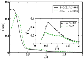
Figure 5: (color online). The frequency dependence of the thermal conductivity $T^{2}\kappa(\omega)$ is shown for two impurities $S=3/2,2$ with $J^{\prime}/J=0.6,0.5$ and $L=14,13$, respectively. Inset: $T^{2}\kappa_{dc}$ as a function of the coupling $J^{\prime}/J$ for $S=3/2,2$. Results are obtained via ED for $\Delta=1$, $\beta\rightarrow 0$.

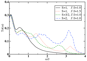
Figure 6: (color online). The frequency dependence of the spin conductivity $T\sigma(\omega)$ is shown for various perturbations: $S=1,3/2,2$ with $J^{\prime}/J=1.0$ and $L=15,14,13$, respectively, as well as the case $S=1$, $L=15$ with $J^{\prime}/J=1.5$. Results are obtained via ED for $\Delta=1$, $\beta\rightarrow 0$.

Another important conclusion that arises from the evaluation of $J^{*}$ is that the larger the $S$ the smaller the $J^{*}$, since $J^{*}\sim 1/\sqrt{S}$. Thus, the local excitations of the impurity dominate even more easily over the bulk contribution for larger $S$. As a matter of fact, we did not obtain a Lorentzian $\kappa(\omega)$ for any $S>1$ by adjusting the host-impurity coupling, implying that any $S>1$ constitutes a strong perturbation for $\kappa(\omega)$ while $S=1$ seems to be quite unique. As far as $\sigma(\omega)$ is concerned, its high frequency regime is dominated by the impurity local excitations, similarly to $\kappa(\omega)$, but its low frequency $\sigma(\omega\rightarrow 0)$ regime remains virtually unaffected for higher $S$. This is a striking difference between $\sigma_{dc}$ and $\kappa_{dc}$ where the former shows a surprising rigidity to the influence of the impurity (large $S$, strong/weak $J^{\prime}$) while the latter is severely reduced in the strong perturbation regime. The above arguments are summarized in Figs. 5, and 6 where the frequency dependence of the thermal, spin conductivity is shown respectively. In Fig. 5, $T^{2}\kappa(\omega)$ is shown for $S=3/2,2$ and $J^{\prime}/J=0.6,0.5$, namely, the corresponding couplings for which $\kappa_{dc}$ is maximum, Fig. 5 inset. For the case of the spin transport we present $T\sigma(\omega)$ in Fig. 6 for various moderate-strong perturbations.

III.3 Lattice size scaling

Let us now turn our attention to the lattice size scaling. A Lorentzian $\kappa(\omega)$ trivially obeys a universal $L$ scaling, with the size independent quantity to be $\kappa(\omega L)/L$, since $\kappa_{dc},\tau^{\epsilon}\sim L$, Fig. 3.Metavitsiadis et al. (2010) On the other hand, for strong $J^{\prime}$, $\kappa(\omega)$ exhibits two $L$-scalings; the prominent impurity contribution at $\omega\sim J^{\prime}$, which is $\mathcal{O}(1)$, does not scale with $L$, Fig. 4(a), while the low frequency bulk contribution obeys the proposed scaling for any $J^{\prime}$. Moreover, in accord with the evaluation of $J^{*}$ (Eq. (7)), Fig. 4(a) shows that the contribution of a single impurity dwindles with respect to the bulk contribution with increasing $L$, becoming negligible in the limit $L\rightarrow\infty$. However, considering the thermodynamic limit and a finite but dilute impurity concentration $c_{I}$—which actually would be a more pragmatic approach to a real system—one could plausibly assume that the high frequency structure will be present, and similar scaling behaviors would hold with the substitution $1/L\rightarrow c_{I}$.

IV Strong coupling limit

Figure 7: The energy spectrum of the isotropic 3-spin system, Eq. (8).

Interesting conclusions can be reached in the strong host-impurity limit, $J^{\prime}\rightarrow\infty$, and are rather useful to understand the high frequency behavior of $\kappa(\omega)$, $\sigma(\omega)$. Starting from Eq. (1) for the isotropic point ($\Delta=1$) and taking $J=0$, we end up in the Hamiltonian of a 3-spin system

$$\mathcal{H}=J^{\prime}(\mathbf{s}_{L-1}+\mathbf{s}_{1})\cdot\mathbf{S}\>.$$ (8)

Exploiting the rotational symmetry and the limited degrees of freedom of $\mathcal{H}$, we perform an analytical diagonalization into different $S_{z}$-total subsectors. The lowest/highest $|S_{z}|=S+1$ subsectors are $\mathcal{D}=1$ Hilbert spaces. The second lowest/highest $|S_{z}|=S$ subsectors are $\mathcal{D}=3$ Hilbert spaces. The rest $2\mathcal{S}+1$ $S_{z}$ subsectors, with $\mathcal{S}=S-1$, are $\mathcal{D}=4$ Hilbert spaces. The energy spectrum of the 3-spin system is shown in Fig. 7.

Considering the local energy current operator $\tilde{\jmath^{\epsilon}}=J^{\prime 2}\mathbf{S}\cdot(\tilde{\mathbf{s}}_{1}\times\tilde{\mathbf{s}}_{L-1})$, we can see that its matrix elements vanish between non-zero eigenvalues, and, consequently, only transitions between zero and non-zero eigenvalues survive; this holds apart from the isotropic point as well. Particularly, for the isotropic Heisenberg model, the only non-vanishing transitions correspond to an energy difference $\delta\epsilon=\pm J^{\prime}$. Thus, for $\Delta=1$, $\kappa(\omega)$ will exhibit only one sharp peak at high frequencies located at $\omega\simeq J^{\prime}$ and it will be independent of $S$. Transitions corresponding to $\delta\epsilon=\pm J^{\prime}$ are between elevated eigenstates, Fig. 7, thus the peak at $\omega\simeq J^{\prime}$ is expected to diminish with decreasing temperature and finally to vanish as the system flows towards its ground state. These selection rules do not hold for the spin transport where there are more allowed transitions. These transitions involve the ground state $\epsilon_{g}$ as well and consequently resonant peaks will be present at low $T$. Lastly, for $\Delta\neq 1$ there are transitions of $\tilde{\jmath^{\epsilon}}$ which do not necessarily correspond to $\delta\epsilon=\pm J^{\prime}$ and yield a more complicated high frequency structure for $\kappa(\omega)$.

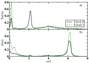
Figure 8: (color online).  a, b) The frequency dependence of the thermal conductivity $T\kappa(\omega)$, spin conductivity $\sigma(\omega)$ respectively for an $S=2$ impurity with $J^{\prime}=2J$, $L=19$, $\Delta=1$ and two temperatures $T/J=0.7,2$. Results are obtained via FTLM.

The previous analytical arguments are verified in Fig. 8 where results are obtained via FTLM for $L=19$ and various perturbations. The frequency dependence of the thermal conductivity $T\kappa(\omega)$ Fig. 8(a) and the spin conductivity $\sigma(\omega)$ Fig. 8(b) is shown, for $S=2$, $J^{\prime}=2J$, $\Delta=1$ at $T/J=0.7,2$.

Starting with Fig. 8(a) we can see that at high temperatures the prevalent contribution to $\kappa(\omega)$ comes from the operator $\tilde{\jmath^{\epsilon}}$ yielding a prominent peak at $\omega=J^{\prime}$ independent of $S$ (compare Figs. 4(b) and 8(a)). As the temperature decreases and the system flows to its ground state the peak at $\omega=J^{\prime}$ decreases gradually and eventually vanishes. Note that the high frequency leap in Fig. 8(a), present at $T/J=0.7$, emerges from $\propto JJ^{\prime}$ terms of the $\jmath^{\epsilon}$ current, Eq. (3). In contrast to the thermal transport, the local excitations of the spin current in the reduced system, Eq. (8), involve the ground state giving a sharp peak at $\omega=J^{\prime}(S+1)$ which does not vanish with decreasing temperature, Fig. 8(b).

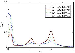
Figure 9: (color online). The frequency dependence of the normalized thermal conductivity $\bar{\kappa}(\omega)$ for $S=1$, $J^{\prime}=2J$, $L=19$ and $\Delta=\pm 0.5$ at $T/J=0.7,50$. Results are obtained via FTLM.

In Fig. 9 we present the normalized thermal conductivity $\bar{\kappa}(\omega)$ for $S=1$, $J^{\prime}=2J$, $\Delta=\pm 0.5$ at $T/J=0.7,50$; results are obtained via FTLM for $L=19$. First, in connection with the previous arguments, we can say that the complicated high frequency structure of $\kappa(\omega)$ for $\Delta\neq 1$ indicates that the single excitation at $\omega=J^{\prime}$ is a unique property of the isotropic Heisenberg model. Second, we focus on the low frequency part of $\kappa(\omega)$ and particularly on the stark difference for $\Delta\lessgtr 0$ at low temperatures. The chain exhibits cutting(healing) behavior for $\Delta>0$($\Delta<0$) for an $S=1$ impurity embedded in the chain which was previously reported for an $S=\frac{1}{2}$ impurity out of the chain.Furusaki and Hikihara (1998); Metavitsiadis et al. (2010) At high temperatures the curves for $\Delta=\pm 0.5$ are one on top of the other. As the temperature decreases, $\kappa(\omega)$ for $\Delta=-0.5$ tends to obtain a more Lorentzian-like form, characteristic of the weak perturbation regime. On the contrary, for $\Delta=+0.5$, $\kappa(\omega)$ obtains a strongly non-monotonic behavior with decreasing temperature resembling the thermal conductivity of an open chain and signifying the flow to the strong perturbation regime. Note that $\sigma(\omega)$ exhibits a similar low frequency behavior for $\Delta=\pm 0.5$ which could be plausibly read as evidence of a finite $D_{S}$, yielding a $\sim\delta(\omega)$ contribution to $\sigma^{\prime}(\omega)$, in the pure AHM for $|\Delta|<1$.

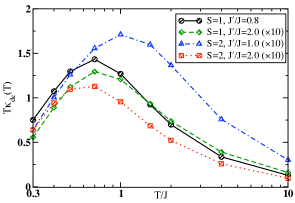
Figure 10: (color online). The temperature dependence of $T\kappa_{dc}(T)$ for $S=1$, $J^{\prime}/J=0.8,2$ and $S=2,J^{\prime}/J=1,2$; results are obtained for $\Delta=1,L=19$ via FTLM.

It is also interesting to present the temperature dependence of the dc value of the thermal conductivity $\kappa_{dc}$ itself since this is a directly measurable quantity in experiments. In Fig. 10, $T\kappa_{dc}(T)$ is shown for four characteristic perturbations and $\Delta=1$. The main conclusion is that the maximum of $\kappa_{dc}$ occurs at different temperatures for different perturbations. Although for $S=1$ the host-impurity coupling quantitatively only affects the behavior of $\kappa_{dc}$ this is not the case for other impurities like the $S=2$ impurity. Generally the maximum of $\kappa_{dc}$ may occur at different temperatures even for the same impurity if this is coupled to the chain with different host-impurity couplings $J^{\prime}$.

Finally, we would like to address the screening of the impurity by the chain which has been discussed previously in the literature.Eggert and Affleck (1992); Mahajan and Venkataramani (2001); Eggert et al. (2001) The ground state of the 3-spin system $\epsilon_{g}$ is $(2\mathcal{S}+1)$-fold degenerate, Fig. 7, implying that the impurity with its neighbors form an effective spin $\mathcal{S}$ at low energies. Thus, for a strong $J^{\prime}$ one can assume that the degrees of freedom of the system at low energies will be described by states of the form $|\epsilon_{g}\rangle\otimes|\psi_{L-3}\rangle$, where the pseudo spin $\mathcal{S}$ couples with the rest of the chain with an effective coupling $\tilde{J}$. $\tilde{J}$ can be evaluated considering the matrix elements of the operator $h_{1}$ at low energies.Zhang et al. (1997) For an $S=2$ impurity we obtain the effective coupling to be ferromagnetic, $\tilde{J}=-0.25J$, while the larger the $S$ the weaker the $\tilde{J}$. Thus, for a single impurity in a finite system, or a finite concentration of impurities in the thermodynamic limit, the picture of the effective spin clearly fails to describe the whole frequency range since the weak $\tilde{J}$, $|\tilde{J}|\ll|J^{\prime}|$, cannot reproduce the high frequency, conspicuous, excitations yielded by a strong $J^{\prime}$ at $\omega\sim J^{\prime}$.

V Discussion and Conclusions

It is worthwhile to devote a few lines to contrast the basic points of the present model, where the impurity is embedded in the chain (IEC), with those of the model studied previously with the impurity located out of the chain (IOC).Metavitsiadis et al. (2010) Stark differences arise in the transport properties of the two models due to the position of the impurity and the way it couples to the pure system. For instance, a weak host-impurity coupling $J^{\prime}$ is a strong perturbation for the IEC model, Fig. 4(b), while taking $J^{\prime}=0$ in the IOC model we end up in the pure AHM. Note also that it would not be accurate to perceive the difference $|J-J^{\prime}|$ as a perturbative parameter, simply, because the case $J^{\prime}=J$ does not correspond to the minimal perturbation of the heat transport. In addition, for different impurities the maximum $\kappa_{dc}$ occurs at different $J^{\prime}$ which does not necessarily correspond to the maximum of $\sigma_{dc}$, Figs. 2, 5 inset. For spin-$S$ impurities with $S>1$ $\kappa(\omega)$ exhibits a non-monotonic form. The absence of a Lorentzian $\kappa(\omega)$ for $S>1$ and any host-impurity coupling $J^{\prime}$ is an indication that $S>1$ impurities constitute a strong perturbation for the heat transport of the Heisenberg model. This is in sharp contrast to the behavior of $\kappa(\omega)$ in the IOC model which obeys a universal scaling with the $\mathcal{B}^{2}$ parameter, at least for weak-intermediate $J^{\prime}$.

Another significant difference between the two models arises from the absence of a $\propto J^{\prime 2}$ term in the energy current of the IOC model. As we have shown in this work, the $\tilde{\jmath^{\epsilon}}$ term accounts for the prominent high frequency excitations which become the prevalent contribution to $\kappa(\omega)$ for strong perturbations. Similarly, the high frequency behavior of $\sigma(\omega)$ for strong perturbations is different in the IEC and the IOC models due to the absence of a perturbative spin current term $\propto J^{\prime}$ in the latter. From all the above one could conclude that the magnetic impurity in the IEC model is a much stronger perturbation for a Heisenberg chain than in the IOC model.

To summarize, studying the thermal $\kappa$ and spin $\sigma$ conductivities of the 1D, spin-$\frac{1}{2}$, AHM with an embedded spin-$S$ impurity at finite temperatures $T$, we have reached the following conclusions: (i) An $S=1$ impurity can be considered as a relatively weak perturbation for some host-impurity couplings $J^{\prime}$, in contrast to $S>1$ impurities which have a more drastic effect on $\kappa$. Furthermore, the difference between $\sigma_{dc}$ and $\kappa_{dc}$ is remarkable since the former shows an impressive rigidity under the influence of the impurity. (ii) $\kappa(\omega)$ obeys a universal scaling $\kappa(\omega L)/L$ for weak and intermediate $J^{\prime}$, while a strong $J^{\prime}$ triggers the emergence of impurity local excitations ruining the $L$-scaling of $\kappa(\omega)$. (iii) We have demonstrated the origin of these resonant modes for a large $J^{\prime}$ and a finite system—their position, their magnitude, and their temperature behavior as well, Eq. (7), Fig. 8. (iv) The presence of these sharp excitations at low $T$ makes the picture of the effective spin $\mathcal{S}=S-1$ insufficient to describe the finite frequency transport properties, Fig. 8—at least for a single impurity in a finite system or plausibly for a finite concentration of impurities in the thermodynamic limit. (v) Finally, we observe the cutting-healing behavior of the chain according to the sign of $\Delta$ as it was previously reported for magnetic impurities out of the chain, Fig. 9.Furusaki and Hikihara (1998); Metavitsiadis et al. (2010)

Acknowledgements.

The author thanks P. Prelovšek and X. Zotos for their overall contribution to this paper. This work was supported by the FP6-032980-2 NOVMAG project.

References

- Zotos and Prelovšek (2004) X. Zotos and P. Prelovšek, in Strong interactions in low dimensions (Springer Netherlands, 2004), pp. 347–382.
- Alvarez and Gros (2002a) J. V. Alvarez and C. Gros, Phys. Rev. Lett. 89, 156603 (2002a).
- Heidrich-Meisner et al. (2002) F. Heidrich-Meisner, A. Honecker, D. C. Cabra, and W. Brenig, Phys. Rev. B 66, 140406 (2002).
- Orignac et al. (2003) E. Orignac, R. Chitra, and R. Citro, Phys. Rev. B 67, 134426 (2003).
- Louis and Gros (2003) K. Louis and C. Gros, Phys. Rev. B 67, 224410 (2003).
- Saito (2003) K. Saito, Phys. Rev. B 67, 064410 (2003).
- Heidrich-Meisner et al. (2005) F. Heidrich-Meisner, A. Honecker, and W. Brenig, Phys. Rev. B 71, 184415 (2005).
- Shimshoni et al. (2003) E. Shimshoni, N. Andrei, and A. Rosch, Phys. Rev. B 68, 104401 (2003).
- Rozhkov and Chernyshev (2005) A. V. Rozhkov and A. L. Chernyshev, Phys. Rev. Lett. 94, 087201 (2005).
- Jung et al. (2006) P. Jung, R. W. Helmes, and A. Rosch, Phys. Rev. Lett. 96, 067202 (2006).
- Karahalios et al. (2009) A. Karahalios, A. Metavitsiadis, X. Zotos, A. Gorczyca, and P. Prelovšek, Phys. Rev. B 79, 024425 (2009).
- Sologubenko et al. (2007) A. V. Sologubenko, T. Lorenz, H. R. Ott, and A. Freimuth, Journal of Low Temperature Physics 147, 387 (2007).
- Hess (2007) C. Hess, The European Physical Journal - Special Topics 151, 73 (2007).
- Otter et al. (2009) M. Otter, V. Krasnikov, D. Fishman, M. Pshenichnikov, R. Saint-Martin, A. Revcolevschi, and P. van Loosdrecht, Journal of Magnetism and Magnetic Materials 321, 796 (2009).
- Saito and Miyashita (2002) K. Saito and S. Miyashita, Journal of the Physical Society of Japan 71, 2485 (2002).
- Eggert et al. (1994) S. Eggert, I. Affleck, and M. Takahashi, Phys. Rev. Lett. 73, 332 (1994).
- Eggert (1996) S. Eggert, Phys. Rev. B 53, 5116 (1996).
- Motoyama et al. (1996) N. Motoyama, H. Eisaki, and S. Uchida, Phys. Rev. Lett. 76, 3212 (1996).
- Sologubenko et al. (2001) A. V. Sologubenko, K. Giannò, H. R. Ott, A. Vietkine, and A. Revcolevschi, Phys. Rev. B 64, 054412 (2001).
- Zotos et al. (1997) X. Zotos, F. Naef, and P. Prelovsek, Phys. Rev. B 55, 11029 (1997).
- Klümper and Sakai (2002) A. Klümper and K. Sakai, Journal of Physics A: Mathematical and General 35, 2173 (2002).
- Sakai and Klümper (2003) K. Sakai and A. Klümper, Journal of Physics A: Mathematical and General 36, 11617 (2003).
- Hlubek et al. (2010) N. Hlubek, P. Ribeiro, R. Saint-Martin, A. Revcolevschi, G. Roth, G. Behr, B. Büchner, and C. Hess, Phys. Rev. B 81, 020405 (2010).
- Eggert and Affleck (1992) S. Eggert and I. Affleck, Phys. Rev. B 46, 10866 (1992).
- Eggert et al. (2001) S. Eggert, D. P. Gustafsson, and S. Rommer, Phys. Rev. Lett. 86, 516 (2001).
- Mahajan and Venkataramani (2001) A. V. Mahajan and N. Venkataramani, Phys. Rev. B 64, 092410 (2001).
- Furusaki and Hikihara (1998) A. Furusaki and T. Hikihara, Phys. Rev. B 58, 5529 (1998).
- Metavitsiadis et al. (2010) A. Metavitsiadis, X. Zotos, O. S. Barišić, and P. Prelovšek, Phys. Rev. B 81, 205101 (2010).
- Kane and Fisher (1992) C. L. Kane and M. P. A. Fisher, Phys. Rev. Lett. 68, 1220 (1992).
- Kubo (1957) R. Kubo, Journal of the Physical Society of Japan 12, 570 (1957).
- Luttinger (1964) J. M. Luttinger, Phys. Rev. 135, A1505 (1964).
- Shastry (2006) B. S. Shastry, Phys. Rev. B 73, 085117 (2006).
- Sirker et al. (2009) J. Sirker, R. G. Pereira, and I. Affleck, Phys. Rev. Lett. 103, 216602 (2009).
- Heidrich-Meisner et al. (2003) F. Heidrich-Meisner, A. Honecker, D. C. Cabra, and W. Brenig, Phys. Rev. B 68, 134436 (2003).
- Benz et al. (2005) J. Benz, T. Fukui, A. Klümper, and C. Scheeren, Journal of the Physical Society of Japan 74S, 181 (2005).
- Steinigeweg and Schnalle (2010) R. Steinigeweg and R. Schnalle, Phys. Rev. E 82, 040103 (2010).
- Alvarez and Gros (2002b) J. V. Alvarez and C. Gros, Phys. Rev. Lett. 88, 077203 (2002b).
- Shastry and Sutherland (1990) B. S. Shastry and B. Sutherland, Phys. Rev. Lett. 65, 243 (1990).
- Zotos and Prelovšek (1996) X. Zotos and P. Prelovšek, Phys. Rev. B 53, 983 (1996).
- Peres et al. (1999) N. M. R. Peres, P. D. Sacramento, D. K. Campbell, and J. M. P. Carmelo, Phys. Rev. B 59, 7382 (1999).
- Narozhny et al. (1998) B. N. Narozhny, A. J. Millis, and N. Andrei, Phys. Rev. B 58, R2921 (1998).
- Barišić et al. (2009) O. S. Barišić, P. Prelovšek, A. Metavitsiadis, and X. Zotos, Phys. Rev. B 80, 125118 (2009).
- Long et al. (2003) M. W. Long, P. Prelovšek, S. El Shawish, J. Karadamoglou, and X. Zotos, Phys. Rev. B 68, 235106 (2003).
- Jaklič and Prelovšek (2000) J. Jaklič and P. Prelovšek, Advances in Physics 49, 1 (2000).
- Rigol and Shastry (2008) M. Rigol and B. S. Shastry, Phys. Rev. B 77, 161101 (2008).
- Zotos (2004) X. Zotos, Phys. Rev. Lett. 92, 067202 (2004).
- Zhang et al. (1997) W. Zhang, J. Igarashi, and P. Fulde, Physical Review B 56, 654 (1997).