Self-Excited Multifractal Dynamics

Abstract

We introduce the self-excited multifractal (SEMF) model, defined such that the amplitudes of the increments of the process are expressed as exponentials of a long memory of past increments. The principal novel feature of the model lies in the self-excitation mechanism combined with exponential nonlinearity, i.e. the explicit dependence of future values of the process on past ones. The self-excitation captures the microscopic origin of the emergent endogenous self-organization properties, such as the energy cascade in turbulent flows, the triggering of aftershocks by previous earthquakes and the “reflexive” interactions of financial markets. The SEMF process has all the standard stylized facts found in financial time series, which are robust to the specification of the parameters and the shape of the memory kernel: multifractality, heavy tails of the distribution of increments with intermediate asymptotics, zero correlation of the signed increments and long-range correlation of the squared increments, the asymmetry (called “leverage” effect) of the correlation between increments and absolute value of the increments and statistical asymmetry under time reversal.

Strong scientific efforts are aimed at characterizing, understanding, predicting and using the rich intermittent nonlinear dynamics of extended natural and social systems. In the last two decades, significant progress has been achieved through the development of new concepts and tools, in particular those of scaling, multi-scaling and multifractals that emphasize the role of the symmetry of scale invariance, the coexistence of and interplay between multiple scales and the hierarchical organization of fractal singularities. In this vein, the multifractal formalism provides powerful metrics to quantify the complex spatio-temporal fluctuations occurring in such diverse systems as hydrodynamic turbulence (velocity increments and energy dissipation) Frisch (1995), seismicity (stress field and earthquake triggering) Sornette and Ouillon (2005), financial systems (asset returns) Lux (2008), biology (healthy human heart-beat rhythm) Ivanov et al. (1999) and hydrology (river runoffs) Kantelhardt et al. (2006).

Multifractality reflects the presence of both long-range dependence and hierarchical organization at many scales. A particularly important realm of application is to model and explain the long-memory processes occurring in the time domain Beran (1994), such as found in hydrodynamic turbulence Ray et al. (2008), geological, as well as in meteorological and financial time series Mandelbrot (1997). In addition to describing their multifractal scaling characteristics, good models should embody their endogenous origin, i.e., the multifractal properties result from the explicit mechanism that future values of the process are (nonlinearly) influenced by the whole past history. The endogenous self-excited nature of the generating process indeed plays a key role in the self-organization of the complex hierarchy of the energy cascades in turbulence, in the spatio-temporal patterns of seismicity and in investors’ decision making process leading to reflexivity in financial markets, among many others.

Multifractal processes can be considered as the next level of generalization to the Fractional Brownian motion, which obeys mono-scaling characterized by a single Hurst exponent $0<H<1$, which is itself the unique generalization of the Wiener process $W(t)$ (with $\mathrm{E}\big{[}dW\big{]}=0$ and $\mathrm{E}\big{[}dW^{2}\big{]}=dt$), corresponding to the continuous time random walk with the fixed scaling exponent $H=1/2$.

There is a strong interest in developing models and processes endowed with multifractal properties, which started from the initial models proposed by Richardson Richardson (1922) and Kolmogorov Kolmogorov (1941, 1962). A first period can be identified, extending from 1985 to about 1997, characterized by so-called cascade rules for increments of the process under analysis, which led to lognormal multifractal models Arneodo et al. (1998a). This was followed by many extensions (see for instance Kalisky et al. (2005); Kantelhardt et al. (2006)). For financial time series, the direct empirical evidence of a causal hierarchical cascade Arneodo et al. (1998b) motivated future developments. The discrete hierarchical cascade approach had a number of drawbacks, such as absence of time dependence and discreteness of the hierarchy of scales. These drawbacks were solved in part by the introduction of subordinate Wiener processes expressed as functions of a non-decreasing fractal time Mandelbrot (1997) and of continuous multifractal cascade models Muzy and Bacry (2002). The Multifractal Markov Switching Model (MSM) is a significant improvement to cascade models that allows for flexible calibration of the parameters Calvet and Fisher (2004), but has unclear economic or physical underpinning, and a rather artificial discrete hierarchical structure.

The Multifractal Random Walk (MRW) Bacry et al. (2001); Muzy and Bacry (2002) is the only continuous stochastic stationary causal process with exact multifractal properties and Gaussian infinitesimal increments. For this, it is delicately tuned to a critical point associated with logarithmic decay of the correlation function of the log-increment up to an integral scale. As a consequence, the moments of the increments of the MRW process become infinite above some finite order, which depend on the intermittency parameter of the model. Generalizations in terms of log-infinitely divisible multifractal processes built as stochastic integral of infinitely divisible 2D noise Barral and Mandelbrot (2002) provide more general non-linear multifractal spectra with non-Gaussian increments Bacry and Muzy (2003). Rather than insisting on asymptotically exact multifractal properties, the continuous-time Quasi-Multifractal model Saichev and Sornette (2006); Saichev and Filimonov (2007, 2008) is based on the simple observation that exponentials of linear long-memory processes exhibit robust effective multifractality for all practical purpose and for a broad range of parameters, removing the rather artificial tuning to criticality needed in the previous models.

All these models use external innovations without explicit dependence of future values on the past history of the process. This crucial trait makes them fundamentally unsuitable to model the mechanisms underlying the empirical systems mentioned above, whose multifractal fluctuations are believed to be generated endogenously. Indeed, turbulence is such that velocity fluctuations cascade to other velocity fluctuations; Seismicity is predominantly powered by earthquakes that trigger other earthquake; Financial return fluctuations, which are weakly coupled to external news, seem mostly driven by reflexivity Soros (1988). This motivates us to introduce the Self-Excited Multifractal (SEMF) model, as the simplest multifractal process with self-generating properties.

In discrete time $t=0,1,2,...,n,...$ (denoting without loss of generality the time increment $\delta t\to 1$), the SEMF process reads $X_{n}=\sum_{i=0}^{n}d_{i}$, where its increments are given by the following recurrence relation

$$d_{n}=\sigma\xi_{n}\exp\left\{-\frac{\omega_{n}}{\sigma}\right\},\quad\omega_{n}=\sum_{i=0}^{n-1}d_{i}h_{n-i-1}~{}.$$ (1)

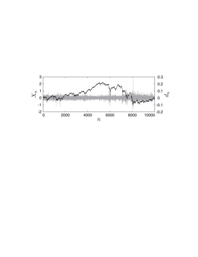
The random variables $\xi_{n}$ represent an external noise, here taken i.i.d. Gaussian with zero-mean and unit variance. The parameter $\sigma$ sets the impact amplitude of the external noise, as well as the dimension and scale of $d_{n}$ and $X_{n}$. Its value determines the time scale. The sum in the exponential expresses the fact that the amplitude of the next increment of the SEMF process is strongly determined by its past realizations, weighted by the memory kernel $h_{i}\geq 0,i=0,...,n-1$, making the dynamics “self-excited”. Fig. 1 shows a typical realization of the increments $d_{n}$ defined by (1) and of the process $X_{n}=\sum_{i=0}^{n}d_{i}$ with the power-law kernel

$$h_{n}=h_{0}n^{-\varphi-1/2}.$$ (2)

In the paper we will also consider the exponentially decaying kernel

$$h_{n}=h_{0}\exp\left(-\phi n\right)$$ (3)

and the constant kernel $h_{n}\equiv h_{0}$, where $\varphi$, $\phi$ and $h_{0}$ are positive constants.

Figure 1: Time-series of increments $d_{n}$ (gray) and values $X_{n}=\sum_{i=0}^{n}d_{i}$ (black) of the discrete SEMF process defined by (1), for $\sigma=0.01$ and with the power-law kernel (2) with $\varphi=0.01,~{}h_{0}=0.05$.

The continuous-time version of the SEMF process is formally defined by the stochastic integro-differential equation in the Ito sense

$$dX(t)=\sigma\exp\left\{-\frac{1}{\sigma}\int\limits_{-\infty}^{t}h(t-t^{\prime})dX(t^{\prime})\right\}dW(t),$$ (4)

where $dW(t)$ is the increment of the regular Wiener process and $h(t)$ is a memory kernel function. The issue of existence of a solution to (4) in the strong or weak sense is considered elsewhere. For our present purpose, it is sufficient to justify expression (4) as the formal notation of the discrete formulation (1) in the limit where the time increment $\delta t$ goes to zero. This limit corresponds to taking $\sigma\to 0$ appropriately ($\sigma\simeq\sqrt{\delta t}$ for the special limiting case $h(t)=0$ retrieving the standard random walk).

The discrete SEMF process can be considered as the simplest multifractal generalization of the GARCH process Bollerslev et al. (1992). It can also be viewed as a simplified time-only continuous or discrete variant of the multifractal stress activation model introduced earlier to model earthquake rupture processes Sornette and Ouillon (2005). Interpreting the increments (1) of the SEMF process as returns of a financial time series, the random variables $\xi_{n}$’s represent an external flow of news, which can be either positive or negative, and which controls the signs of the returns. The amplitude (or volatility) of the returns are then determined by all past returns with a decaying weight as a function of their distance to the present.

The previously mentioned multifractal models require stringent conditions on their memory structure in order to exist, that is, for their construction to converge. For instance, the MRW can be expressed in the form (4) but with the $dX(t^{\prime})$ in the integral in the exponential replaced by an external random Wiener increment and, crucially, with $h(t)\sim 1/\sqrt{t}$ up to an integral time scale and $h(t)=0$ beyond. Slower decaying kernels make the construction non-convergent. Faster decaying kernels destroy multifractality. The Quasi-Multifractal model Saichev and Sornette (2006); Saichev and Filimonov (2007) generalizes the MRW by using a power law kernel $h(t)=h_{0}/\left(1+t/\tau\right)^{\varphi+1/2}$, and exists only for $\varphi>0$.

In contrast, the SEMF process is much more robust and enjoy a large domain of existence, for almost arbitrary specifications of the memory kernel. Consider for instance the extreme case of a permanent memory $h(t)\equiv h_{0}>0$.Then, expression (4) becomes

$$dX=\sigma e^{-(h_{0}/\sigma)X}dW.$$ (5)

Using the Lamperti transformation Jeanblanc et al. (2009) $Z={1\over h_{0}}e^{h_{0}X/\sigma}$, and Ito’s lemma, equation (5) leads to $dZ={1\over 2}{1\over Z}dt+dW$, whose solution is the two-dimensional Bessel process

$$B_{2}(t)=\sqrt{[W_{1}(t)]^{2}+[W_{2}(t)]^{2}},$$ (6)

where $W_{1}(t)$ and $W_{2}(t)$ are two independent Wiener processes. Thus,

$$X(t)={\sigma\over h_{0}}\ln\left[h_{0}B_{2}(t)\right].$$ (7)

Since, $B_{2}(t)$ does not reach $0$ almost surely in finite time and does not exhibit a finite-time singularity Jeanblanc et al. (2009), the process $X(t)$ is also well-behaved. The statistic properties of the increments of the SEMF process (7) with constant kernel can then be obtained from the exact solution (7) and will be reported elsewhere.

In general, the SEMF processes do not have stationary increments both in discrete or continuous time, except for the trivial case $h_{0}=0$ which recovers the simple Wiener process. The case of a constant memory kernel leading to the solution (7) is a good illustration. In addition to controlling the multifractality and other important properties, the amplitude $h_{0}$ in (2) and (3) can be considered as a “measure of non-stationarity” of the increments. Such non-stationarity might be seen as a deficiency. However, we argue that models that enforce stationarity of increments for the convenience of their analysis may actually miss the genuine non-stationarity nature of many natural and social dynamics. Let us mention in physics the case of freely decaying two- and three-dimensional turbulence Eyink and Thomson (2000). In finance, there is strong evidence supporting the view that stock market returns are non-stationary, subjected to regime shifts Woodward and Anderson (2009) which can be transitory or permanent MacKenzie (2008).

One of the mechanisms at the source of non-stationarity in SEMF processes is the rare occurrence of extreme events, as illustrated by a single realization shown in Fig. 2. Notice the sharp growth of the volatility followed by a collapse and a very long recovery. In the discrete version (1), this results from rare long runs of negative innovations $\xi_{n}$ following by a sign reversal. The exact relation between the mean time for recovery to the size of the burst depends on the shape of the kernel. Simulations show that the mean time for recovery increases faster than exponentially with the burst size for power-law kernels (2). These extreme events are responsible for the extremely long tail of the probability density function of increments shown in figure 5 below, exemplifying the “dragon-king” phenomenon Sornette (2009). Given the extreme impact of these events, it is natural both from a mathematical point of view and motivated by empirical evidence to enrich the SEMF model with a “stop and resume” rule leading to a standard renewal process (see Feller (1968)), making the renewal SEMF model having stationary increments. In the sequel, we do not explore this extension and stick to the SEMF process (1) with the “measure of non-stationarity” $h_{0}<0.2$, such that the probability of occurrence of extreme events in time series of duration $N=10^{5}$ is smaller than $10\%$. The reported statistical properties are averaged over the realizations which do not exhibit these extreme bursts.

Figure 2: An extreme event in the increments of the discrete SEMF process.

Let consider the multifractal properties of the SEMF process. To remove possible biases stemming from some non-stationary features of the increments of SEMF processes, we used the multifractal detrended fluctuation analysis (MF-DFA) Kantelhardt et al. (2002) to calculate the q-th order fluctuation function

$$F_{q}(s)=\left\{\frac{1}{2N_{s}}\sum_{\nu=1}^{2N_{s}}\big{[}F^{2}(\nu,s)\big{]}^{q/2}\right\}^{1/q},$$ (8)

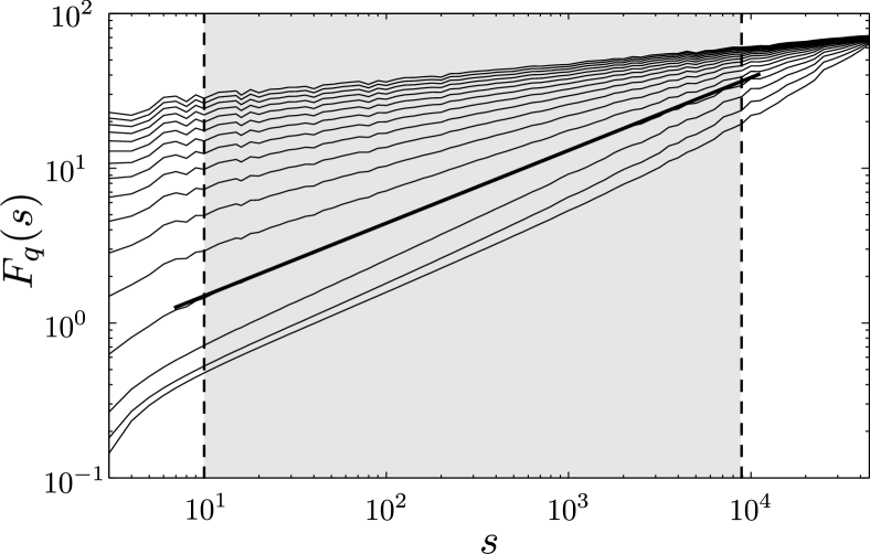
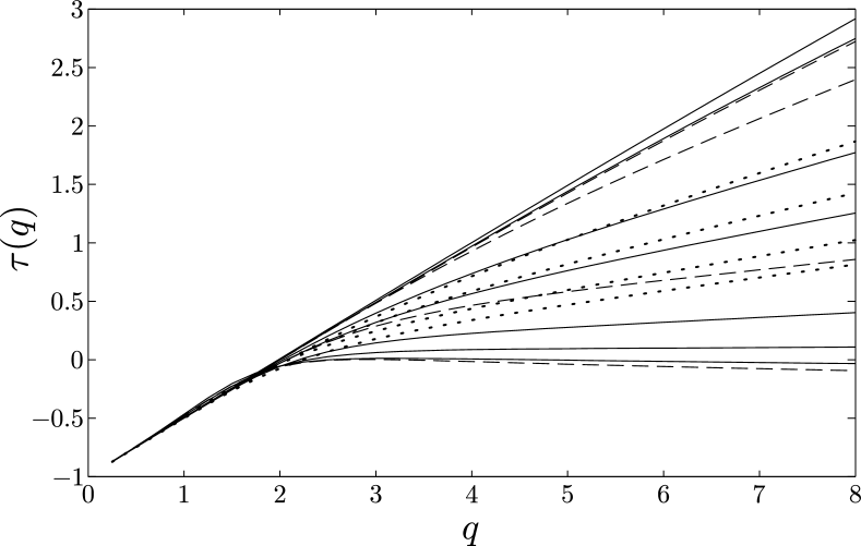
where $N_{s}$ is a number of segments of length $s$ within the whole time-series $X_{n}$ of length $N=10^{5}$ and $F^{2}(\nu,s)$ is the averaged squared residuals of the linear fit of the time series $X_{n}$ within the time segment $\nu$. To remove transient effects, we remove the first half of the generated time series, i.e., we considered $X_{n}$ for $N/2\leq n\leq N$. Fig. 3 presents the q-th order fluctuation functions for 16 different values of the order $q$, averaged over $M=1000$ realizations of the SEMF process. For $10<s<N/10$, one can observe an excellent scaling regime $F_{q}(s)\sim s^{h(q)}$, where the exponents $h(q)$ are the slopes in the grey area of Fig. 3. The scaling exponent $\tau(q)$ of the standard multifractal structure function is obtained from the generalized Hurst exponent $h(q)$ by using the relationship $\tau(q)=qh(q)-1$. The non-linear dependence of the exponents $\tau(q)$ as a function of the order $q$ shown in Fig. 4 characterizes the multifractal properties of the process for different memory kernels, which include the power law (2), exponential (3) and the constant kernel $h_{n}\equiv h_{0}$. SEMF process is found to exhibit multifractal scaling over large intermediate range of scales. The parameter $h_{0}$ controls the level of multifractality: increasing $h_{0}$ changes the spectrum from nearly monofractal for small $h_{0}$ values to strongly multifractal.

Figure 3: Log-log plot of the averaged fluctuations function given by (8) as a function of scale $s$, for $q=0.5n$, $n=1$ to $16$ (bottom to top), for $\sigma=1$ and power-law kernel (2) with $\varphi=0.1$ and $h_{0}=0.16$. The grey rectangle delineates the range of scales where the fluctuation function was approximated with a strict power-law $F_{q}(s)=K_{q}s^{h(q)}$. The bold line shows the power-law approximation for the case $q=2$.

Figure 4: Multifractal scaling exponents $\tau(q)$ of the process $X_{n}$ for $\sigma=1$ and (i) power-law kernel (2) with $\varphi=0.01$ and $h_{0}=0.01,~{}0.06,~{}0.08,~{}0.10,~{}0.12,~{}0.14,~{}0.16$ (solid lines top to bottom), (ii) exponential kernel (3) with $\phi=0.01$ and $h_{0}=0.06,~{}0.08,~{}0.10,~{}0.12$ (dotted lines top to bottom), (iii) constant kernel $h\equiv h_{0}=0.02,~{}0.04,~{}0.06,~{}0.08$ (dashed lines top to bottom).

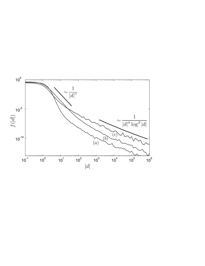
The probability density function (pdf) $f(d)$ of the increments exhibits a heavy tail, as shown in Fig. 5. Using a large statistics of $M=10^{8}$ time-series of $10^{3}$ discrete time steps for each of the three types of kernels (power-law, exponential and constant), we observe three regimes for the pdf: (i) a plateau for small $d$’s, an intermediate asymptotic for $2\sigma\lesssim d\lesssim 20\sigma$ in the form of an approximate power law

$$f_{d}(d)\sim\frac{1}{d^{\gamma}},$$ (9)

where $2\lesssim\gamma\lesssim 6$, and (iii) a very long tail

$$f_{d}(d)\sim\frac{1}{d^{\alpha}\log^{\beta}d},$$ (10)

where $\alpha\sim 1$ and $\beta\sim 2$. The specific values of the exponents $\alpha,~{}\beta,~{}\gamma$ depend on the functional shape of the kernel $h_{n}$. For instance, for the power-law kernel (2) with $\varphi=0.01,~{}h_{0}=0.14$, we obtain $\alpha=0.8,~{}\beta=4.2$ and $\gamma=4.6$. Within the financial interpretation, choosing $\sigma\approx 1\%$ (corresponding roughly to a time scale $\delta t\simeq 1$ day), the intermediate power law asymptotics recovers the empirical power law distribution with an exponent often reported in the range $3\leq\gamma\leq 5$ for returns in the return amplitude range $1-20\%$ Cont (2001). The extreme tail (10) may correspond to the “dragon-king” regime Sornette (2009), resulting from amplifying mechanisms leading to rare transient huge bursts. This tail can be derived analytically using large deviation methods, as will be reported elsewhere. Intuitively, exponentially rare streams of negative innovations $\xi_{k}$ give rise to explosive growth of $d_{n}$, until a positive $\xi_{j}$ occurs leading to a collapse of the next increment $d_{j+1}$. The dynamics of the SEMF process is thus characterized by quasi-stationary very long regimes punctuated by rare bursts and collapses that play special roles, not unlike coherent structures in turbulence or bubbles and crashes in financial markets. The study of these special properties will be reported elsewhere.

Figure 5: Probability density function of the absolute values of the increments $d_{n}$ for $\sigma=1$: (a) power-law kernel (2) with $\varphi=0.1,~{}h_{0}=0.1$, (b) constant kernel $h_{n}=h_{0}=0.02$ and (c) exponential kernel (3) with $\phi=0.01,~{}h_{0}=0.1$.

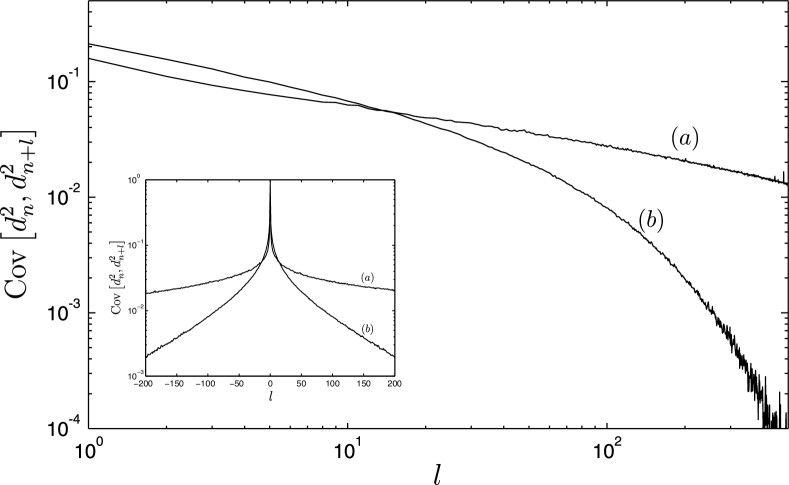
The SEMF process exhibits a very long dependence between the absolute value of its increments and no dependence between the increments themselves due to the i.i.d. random variables $\xi_{n}$. The former property can be quantified by the covariance coefficient $\text{Cov}\left[d^{2}_{n},d^{2}_{n+l}\right]$. Conditioning our estimation of this covariance coefficient by excluding the rare occurrences of the huge explosive bursts at the origin of the very heavy tail (10), we obtain the results shown in fig. 6, again after a statistical averaging over $M=10^{8}$ time-series of length $10^{3}$. The decay of $\text{Cov}\left[d^{2}_{n},d^{2}_{n+l}\right]$ is slower than exponential both for slow power-law (2) and exponential (3) kernels in the range of values $>0.001-0.01$ that is meaningful for empirical data. In the case of the power law kernel, $\text{Cov}\left[d^{2}_{n},d^{2}_{n+l}\right]\simeq 1/l^{\kappa}$, with $\kappa=0.2-0.4$, which is typical of empirical calibration of financial returns.

Figure 6: Covariance coefficient $\text{Cov}\left[d^{2}_{n},d^{2}_{n+l}\right]$ of the squared increments with $n\geq N/2$, $\sigma=1$, for (a) the power-law kernel (2) with $\varphi=0.01,~{}h_{0}=0.08$ and (b) the exponential kernel (3) with $\phi=0.01,~{}h_{0}=0.05$. In this later case, for $l<150$ the covariance decays as a stretched exponential $\exp\left(-0.13\,x^{0.51}\right)$. The inset shows the same data in log-linear scale.

As a bonus, the SEMF process exhibits the so-called leverage effect Bouchaud et al. (2001), defined as a negative correlation between past increments $d_{n}$ and future squared increments $d_{n}^{2}$ of the process and absence of correlation between past $d_{n}^{2}$ and future $d_{n}$. The leverage effect is in general also asymmetric in the effect of the sign of the return $d_{n}$: a large negative return (loss) leads to a significant increase of volatility, while a large positive return (gain) has smaller impact on the subsequent volatility. Remarkably, the SEMF process captures these effects. Indeed, consider the return $d_{n}$ given by (1) and the subsequent volatility $v_{n+1}$ that has the form:

$$v_{n+1}=\exp\left\{-\frac{\omega_{n+1}}{\sigma}\right\}=\exp\left\{-\frac{1}{\sigma}\sum_{i=0}^{n-1}d_{i}h_{n-i}-h_{0}d_{n}\right\}.$$

The impact of the increment $d_{n}$ on $v_{n+1}$ is exponential with a negative sign. Due to the convexity of the exponential function, the relative increase ($|v_{n+1}-v_{n}|/v_{n}$) of the volatility following a loss $d_{n}<0$ is larger than the relative decrease of the volatility after a gain $d_{n}>0$. Moreover, the larger the previous loss/gain, the larger is the subsequent relative volatility increase/decrease.

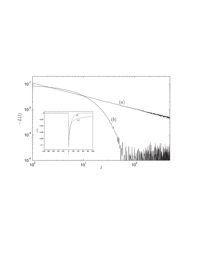
The leverage effect can be quantified by the normalized correlation function $L(l)=\mathrm{E}\Big{[}d_{n}d_{n+l}^{2}\Big{]}/\left(\mathrm{E}\Big{[}d_{n}^{2}\Big{]}\right)^{3/2}$, which should be equal to zero for $l<0$ and negative for $l>0$ for the effect to be present. For the SEMF process (1), the function $L(l)$ has the form:

$$L(l)=\frac{\mathrm{E}\left[\xi_{n}\xi^{2}_{n+l}e^{-(\omega_{n}+2\omega_{n+l})/\sigma}\right]}{\Big{(}\mathrm{E}\left[\xi_{n}^{2}e^{-2\omega_{n}/\sigma}\right]\Big{)}^{3/2}}.$$ (11)

For $l<0$, $\omega_{n}$ and $\omega_{n+l}$ do not depend on the random variable $\xi_{n}$, leading to $L(l)=0$. For $l>0$, we find analytically that the function (11) is negative ($L(l)<0$), which proves the presence of the leverage effect in the SEMF model. Fig. 7 illustrates this result by plotting the function $L(l)$ obtained by averaging over a set of $M=10^{8}$ time-series of length $10^{3}$ generated by the SEMF process with the power-law (2) and exponential (3) memory kernels. One verifies the defining asymmetry of the leverage effect. It also should be noted that the shape of function $L(l)$ for $l>0$ corresponds to the shape of memory kernel $h_{n}$.

Figure 7: Leverage coefficient $L(l)$ defined in (11) for the process $X_{n}$ with $\sigma=1$ for (a) the power-law kernel (2) with $\varphi=0.01,~{}h_{0}=0.05$ and (b) the exponential kernel (3) with $\phi=0.1,~{}h_{0}=0.04$. The shape of $L(l)$ for $l>0$ is (a) power-law $L(l)\simeq-l^{-0.51l}$ and (b) exponential $L(l)\simeq-\exp(-0.1l)$.

Finally, we document a very interesting property of the SEMF process, namely the breaking of statistical time reversal symmetry, that arises naturally from its self-excitated structure, and which is related to the leverage effect. In contrast, the MRW Bacry et al. (2001); Muzy and Bacry (2002) and the Quasi-Multifractal Saichev and Sornette (2006); Saichev and Filimonov (2007, 2008) processes possess the property of statistical time reversal symmetry. The breaking of statistical time-reversal symmetry is a stylized fact of chaotic dynamics, turbulence and self-organized (critical or not) systems Sornette (2006). In particular, financial time-series are characterized by a breaking of statistical time-reversal symmetry Ramsey and Rothman (1996); Arneodo et al. (1998c). In the SEMF model, the breaking of the time-reversal symmetry is already obvious from visual inspection of figure 2, when an extreme event in the increments of the discrete SEMF process occurs. Quantitatively, the three -point covariance function $C_{3}(\tau)=\mathrm{E}\big{[}X_{n}(X_{n+2\tau}-X_{n+\tau})X_{n+3\tau}\big{]}$ introduced by Pomeau Pomeau (1982) provides one of its possible diagnostic. For $\tau=1$, we find that

$$C_{3}(1)=\sigma^{3}\sum_{i=0}^{n}\sum_{j=0}^{n+3}\mathrm{E}\Big{[}\xi_{i}\xi_{j}\xi_{n+2}e^{-(\omega_{i}+\omega_{j}+\omega_{n+2})/\sigma}\Big{]}\neq 0~{}.$$ (12)

Because the mean under the sum is non-zero only for $j=n+2$, this leads to

$$C_{3}(1)=\sigma^{3}\sum_{i=0}^{n}\mathrm{E}\Big{[}\xi_{i}\xi^{2}_{n+2}e^{-(\omega_{i}+2\omega_{n+2})/\sigma}\Big{]}~{}.$$ (13)

The mean value under the sum sign has the form of the numerator of the expression giving the leverage coefficient (11) with $l=n+2-i>0$, which is found negative both in our analytical and numerical calculations. This implies that $C_{3}(1)<0$ and proves the breaking of statistical time reversal symmetry in the SEMF processes.

Summarizing, we have introduced the self-excited multifractal (SEMF) process that exhibits strong multifractal properties with an explicit dependence of the dynamics of the process on both external events and internal memory. The SEMF process enjoys all the stylized facts of self-organizing systems such as turbulent flows, seismicity or financial markets: multifractality, heavy tails of the distribution of increments, absence of correlation of the signed increments and long-range dependence in the squared increments. The “leverage effect” and time-reversal asymmetry are also some of its intrinsic properties. Having the explicit feedback of the past values on the future ones, the SEMF model is a promising candidate for describing critical events in the self-organized systems mentioned above.

We are grateful to Professor Alexander Saichev for fruitful discussions.

References

- Frisch (1995) U. Frisch, Turbulence (Cambridge University Press, Cambridge, 1995).
- Sornette and Ouillon (2005) D. Sornette and G. Ouillon, Phys. Rev. Lett. 94, 038501+ (2005).
- Lux (2008) T. Lux, J. Bus. Econ. Stat. 26, 1 (2008).
- Ivanov et al. (1999) P. C. Ivanov, L. A. Amaral, A. L. Goldberger, S. Havlin, M. G. Rosenblum, Z. R. Struzik, and H. E. Stanley, Nature 399, 461 (1999).
- Kantelhardt et al. (2006) J. Kantelhardt, E. Koscielny-Bunde, D. Rybski, P. Braun, A. Bunde, and S. Havlin, Journal of geophysical research 111, D01106 (2006).
- Beran (1994) J. Beran, Statistics for Long-Memory Processes (Chapman & Hall/CRC, 1994), 1st ed.
- Ray et al. (2008) S. S. Ray, D. Mitra, and R. Pandit, New J. Phys. 10, 1 (2008).
- Mandelbrot (1997) B. Mandelbrot, Fractals and Scaling In Finance (Springer, 1997), 1st ed.
- Richardson (1922) L. F. Richardson, Weather Prediction by Numerical Process (Cambridge University Press, 1922).
- Kolmogorov (1941) A. N. Kolmogorov, Dokladi Akademii Nauk SSSR XXXI, 299 (1941).
- Kolmogorov (1962) A. N. Kolmogorov, Journal of Fluid Mechanics 13, 82 (1962).
- Arneodo et al. (1998a) A. Arneodo, E. Bacry, and J. Muzy, J. Math. Phys. 39, 4142 (1998a).
- Kalisky et al. (2005) T. Kalisky, Y. Ashkenazy, and S. Havlin, Physical Review E 72, 011913 (2005).
- Arneodo et al. (1998b) A. Arneodo, J. Muzy, and D. Sornette, European Physical Journal B 2, 277 (1998b).
- Muzy and Bacry (2002) J. F. Muzy and E. Bacry, Phys. Rev. E 66, 056121 (2002).
- Calvet and Fisher (2004) L. E. Calvet and A. J. Fisher, J. Fin. Econometrics 2, 49 (2004).
- Bacry et al. (2001) E. Bacry, J. Delour, and J. F. Muzy, Phys. Rev. E 64, 026103 (2001).
- Barral and Mandelbrot (2002) J. Barral and B. B. Mandelbrot, J. Prob. Th. Rel. Fields 124, 409 (2002).
- Bacry and Muzy (2003) E. Bacry and J. Muzy, Comm. Math. Phys. 236, 449 (2003).
- Saichev and Sornette (2006) A. Saichev and D. Sornette, Phys. Rev. E 74, 011111+ (2006).
- Saichev and Filimonov (2007) A. Saichev and V. Filimonov, J. Exp. Theor. Phys. 105, 1085 (2007).
- Saichev and Filimonov (2008) A. Saichev and V. Filimonov, J. Exp. Theor. Phys. 107, 324 (2008).
- Soros (1988) G. Soros, The Alchemy of Finance (Simon & Schuster, 1988), 1st ed.
- Bollerslev et al. (1992) T. Bollerslev, R. Chou, and K. Kroner, J. Econometrics 52, 5 (1992).
- Jeanblanc et al. (2009) M. Jeanblanc, M. Yor, and M. Chesney, Mathematical methods for financial markets (Springer-Verlag, London, 2009), 1st ed.
- Eyink and Thomson (2000) G. L. Eyink and D. J. Thomson, Physics of Fluids 12, 477 (2000).
- Woodward and Anderson (2009) G. Woodward and H. Anderson, Quantitative Finance 9, 913 (2009).
- MacKenzie (2008) D. MacKenzie, An Engine, Not a Camera: How Financial Models Shape Markets (The MIT Press, 2008), ISBN 0262633671.
- Sornette (2009) D. Sornette, Int. J. Terraspace Sci. Eng. 2, 1 (2009).
- Feller (1968) W. Feller, An Introduction to Probability Theory and Its Applications, vol. 1 (Wiley, 1968), 3rd ed., ISBN 0471257087.
- Kantelhardt et al. (2002) J. W. Kantelhardt, S. A. Zschiegner, E. Koscielny-Bunde, S. Havlin, A. Bunde, and H. E. E. Stanley, Physica A 316, 87 (2002).
- Cont (2001) R. Cont, Quantitative Finance 1, 223 (2001).
- Bouchaud et al. (2001) J.-P. Bouchaud, A. Matacz, and M. Potters, Phys. Rev. Lett. 87, 228701 (2001).
- Sornette (2006) D. Sornette, Critical Phenomena in Natural Sciences. Chaos, Fractals, Selforganization and Disorder: Concepts and Tools (Springer, 2006), 2nd ed., ISBN 3540308822.
- Ramsey and Rothman (1996) J. B. Ramsey and P. Rothman, Journal of Money, Credit and Banking 28, pp. 1 (1996), ISSN 00222879.
- Arneodo et al. (1998c) A. Arneodo, J.-F. Muzy, and D. Sornette, The European Physical Journal B 2, 277 (1998c).
- Pomeau (1982) Y. Pomeau, J. Physique 43, 859 (1982).