Error Estimates for Gaussian Beam Superpositions

Abstract

Gaussian beams are asymptotically valid high frequency solutions to hyperbolic partial differential equations, concentrated on a single curve through the physical domain. They can also be extended to some dispersive wave equations, such as the Schrödinger equation. Superpositions of Gaussian beams provide a powerful tool to generate more general high frequency solutions that are not necessarily concentrated on a single curve. This work is concerned with the accuracy of Gaussian beam superpositions in terms of the wavelength $\varepsilon$. We present a systematic construction of Gaussian beam superpositions for all strictly hyperbolic and Schrödinger equations subject to highly oscillatory initial data of the form $Ae^{i\Phi/\varepsilon}$. Through a careful estimate of an oscillatory integral operator, we prove that the $k$-th order Gaussian beam superposition converges to the original wave field at a rate proportional to $\varepsilon^{k/2}$ in the appropriate norm dictated by the well-posedness estimate. In particular, we prove that the Gaussian beam superposition converges at this rate for the acoustic wave equation in the standard, $\varepsilon$-scaled, energy norm and for the Schrödinger equation in the $L^{2}$ norm. The obtained results are valid for any number of spatial dimensions and are unaffected by the presence of caustics. We present a numerical study of convergence for the constant coefficient acoustic wave equation in $\mathbb{R}^{2}$ to analyze the sharpness of the theoretical results.

1 Introduction

In simulations of high frequency wave propagation, a large number of grid points is needed to resolve and maintain an accurate in time representation of the wave field. Consequently, in this regime, direct numerical simulations are computationally expensive and at sufficiently high frequencies, such simulations are no longer feasible. To circumvent this difficulty, approximate high frequency asymptotically valid methods are often used. One such popular approach is geometrical optics [7, 33], which is obtained in the limit when the frequency tends to infinity. This method is also known as the WKB method or ray-tracing. The solution of the partial differential equation (PDE) is assumed to be of the form

$${}a(t,y,\varepsilon)e^{i\phi(t,y)/\varepsilon},$$ (1)

where $1/\varepsilon$ is the large high frequency parameter, $\phi$ is the phase, and $a$ is the amplitude of the solution having the Debye expansion in terms of $\varepsilon$, $a(t,y,\varepsilon)=\sum_{j=0}^{N}\varepsilon^{j}a_{j}(t,y)$. The phase and amplitudes $a_{j}$ are independent of the frequency and vary on a much coarser scale than the full wave solution. They can therefore be computed at a computational cost independent of the frequency. However, the geometrical optics approximation breaks down at caustics, where rays concentrate and the predicted amplitude is unbounded [24, 19]. The consideration of difficulties caused by caustics, beginning with Keller in [16] and Maslov and Fedoriuk (see [25]), led to the development of the theory of Fourier integral operators, e.g., as given by Hörmander in [10].

Gaussian beams form another high frequency asymptotic model which is closely related to geometrical optics. However, unlike geometrical optics, Gaussian beams do not breakdown at caustics. For Gaussian beams, the solution is also assumed to be of the geometrical optics form (1), but a Gaussian beam is a localized solution that concentrates near a single ray of geometrical optics in space-time. Although the phase function is real-valued along the central ray, Gaussian beams have a complex-valued phase function off their central ray. The imaginary part of the phase is chosen such that the solution decays exponentially away from the central ray, maintaining a Gaussian-shaped profile. To form a Gaussian beam solution, we first pick a ray and solve a system of ordinary differential equations (ODEs) along it to find the values of the phase, its first and second order derivatives and the amplitude on the ray. To define the phase and amplitude away from this ray to all of space-time, we extend them using a Taylor expansion. Heuristically speaking, along each ray we propagate information about the phase and amplitude and their derivatives that allows us to reconstruct the wave field locally in a Gaussian envelope. The existence of Gaussian beam solutions has been known since sometime in the 1960’s, first in connection with lasers, see Babič and Buldyrev [2]. Later, they were used in the analysis of propagation of singularities in partial differential equations by Hörmander [11] and Ralston [30].

In this article, we are interested in the accuracy of Gaussian beam solutions to $m$-th order linear, strictly hyperbolic PDEs with highly oscillatory initial data of the type

$${}Pu =0,\qquad(t,y)\in(0,T]\times\mathbb{R}^{n},$$ (2)

$$\partial_{t}^{\ell}u(0,y) =\varepsilon^{-{\ell}}\sum_{j=0}^{N}\varepsilon^{j}A_{{\ell},j}(y)e^{i\Phi(y)/\varepsilon}\ ,\qquad{\ell}=0,\ldots,m-1\ ,$$

where the strictly hyperbolic operator, $P$, is defined in Section 2.1, the real valued phase, $\Phi(y)$ belongs to $C^{\infty}(K_{0};\mathbb{R})$ for some compact set $K_{0}\subset\mathbb{R}^{n}$, and the complex valued amplitudes, $A_{{\ell},j}(y)$ belong to $C^{\infty}_{0}(K_{0};\mathbb{C})$. Furthermore, we will assume that $|\nabla\Phi(y)|$ is bounded away from zero on $K_{0}$. As a special case, we include the acoustic wave equation,

$$u_{tt}-c(y)^{2}\Delta u=0,\qquad(t,y)\in(0,T]\times\mathbb{R}^{n}\ ,$$

$$u(0,y)=\sum_{j=0}^{N}\varepsilon^{j}A_{0,j}(y)e^{i\Phi(y)/\varepsilon}\ ,\quad\mbox{and}\quad u_{t}(0,y)=\frac{1}{\varepsilon}\sum_{j=0}^{N}\varepsilon^{j}A_{1,j}(y)e^{i\Phi(y)/\varepsilon}\ .{}$$ (3)

We also treat the dispersive Schrödinger equation,

$${}-i\varepsilon u_{t}-\frac{\varepsilon^{2}}{2}\Delta u+V(y)u =0,\qquad(t,y)\in(0,T]\times\mathbb{R}^{n},$$ (4)

$$u(0,y) =\sum_{j=0}^{N}\varepsilon^{j}A_{j}(y)e^{i\Phi(y)/\varepsilon}\ .$$

As above, we will assume that $\Phi\in C^{\infty}(K_{0};\mathbb{R})$ and $A_{j}\in C^{\infty}_{0}(K_{0};\mathbb{C})$. Furthermore, we assume the potential $V(y)$ is smooth and bounded along with all its derivatives, $\partial_{y}^{\beta}V\in C^{\infty}_{b}(\mathbb{R}^{n})$ for all $\beta$. For the Schrödinger equation, the asymptotic parameter $\varepsilon$ appears in the equation and there is no need to assume the bound on $|\nabla\Phi|$ that is necessary for strictly hyperbolic equations.

Since these partial differential equations are linear, it is a natural extension to consider sums of Gaussian beams to represent more general high frequency solutions that are not necessarily concentrated on a single ray. This idea was first introduced by Babič and Pankratova in [3] and was later proposed as a method for wave propagation by Popov in [28]. The sum, or rather the integral superposition, of Gaussian beams in the simplest first order form can be written as

$${}u_{GB}(t,y)=\left(\frac{1}{2\pi\varepsilon}\right)^{\frac{n}{2}}\int_{K_{0}}a(t;z)e^{i\phi(t,y-x(t;z);z)/\varepsilon}dz\ ,$$ (5)

where $K_{0}$ is a compact subset of $\mathbb{R}^{n}$ and the phase that defines the Gaussian beam is given by

$${}\phi(t,y;z)=\phi_{0}(t;z)+y\cdot p(t;z)+y\cdot\frac{1}{2}M(t;z)y\ .$$ (6)

The real vector $p(t;z)$ is the direction of wave propagation and the matrix $M(t;z)$ has a positive definite imaginary part and it gives Gaussian beams their profile. Extensions of the above superposition are possible in several directions, including using higher order Gaussian beams in the superposition and using a sum of several superpositions to approximate the different modes of wave propagation. Higher order Gaussian beams are created by using an asymptotic series for the amplitude and using higher order Taylor expansions to define the phase and the amplitude functions, see (22) and (23). Also, for higher order beams, a cutoff function (19) is necessary to avoid spurious growth away from the central ray. Superpositions with higher order Gaussian beams have an improved asymptotic convergence rate. For $m$-th order strictly hyperbolic PDEs, which have $m$ pieces of initial data, we use $m$ different Gaussian beam superpositions chosen in such a way so that their sum approximates the initial data. Each of these superpositions corresponds to one of the $m$ distinct modes of wave propagation.

Accuracy studies for a Gaussian beam solution $u_{\rm GB}$ have traditionally focused on how well it asymptotically satisfies the PDE, i.e. the size of the norm of $Pu_{\rm GB}$ in terms of $\varepsilon$. The question of determining the error of the Gaussian beam superposition compared to the exact solution was thought to be a rather difficult problem decades ago, see the conclusion section of the review article by Babič and Popov [4]. However, some progress on estimates of the error has been made in the past few years. This accuracy study was initiated by Tanushev in [34], where a convergence rate was obtained for the initial data. Some earlier results on this were also established by Klimeš in [18]. The part of the error that is due to the Taylor expansion off the central ray was considered by Motamed and Runborg in [27] for the Helmholtz equation. Liu and Ralston [22, 23] gave rigorous convergence rates in terms of $\varepsilon$ for the acoustic wave equation in the scaled energy norm and for the Schrödinger equation in the $L^{2}$ norm. However, the error estimates they obtained depend on the number of space dimensions in the presence of caustics, since the projected Hamiltonian flow to physical space becomes singular at caustics. The superpositions in (5) can also be carried out over both $x$ and $p$ in full phase space through the Hamiltonian map, $(z,p_{0})\to(x(t;z,p_{0}),p(t;z,p_{0}))$, as shown in [22, 23]. In this formulation the Hamiltonian flow is regular and there are no caustics, so we expect to obtain a dimensionally independent error estimate. This has been confirmed for the wave equation by Bougacha, Akian and Alexandre in [5] for the case of initial data based on the Fourier–Bros–Iaglonitzer (FBI) transform, a result which is inspired by the work of Rousse and Swart on the Herman-Kluk propagator for the Schrödinger equation [31, 32]. From a computational stand point, the full phase space formulation is more expensive.

Building upon these recent advances, together with an application of a non-squeezing argument proved in Lemma 3, we are able to provide a definite answer to the question of accuracy for Gaussian beam superposition solutions. More precisely, we obtain dimensionally independent estimates for the superposition in physical space for general $m$-th order strictly hyperbolic PDEs and the Schrödinger equation. Our main result is the following theorem.

Theorem 1

Let $u$ be the exact solution to the PDEs considered, (2), (3) and (4), under the stated assumptions on initial data and partial differential operators. Moreover, let $u_{k}$ be the corresponding $k$-th order Gaussian beam superposition given in Section 2.2 and Section 2.3, with a sufficiently small cutoff parameter $\eta$ when $k>1$. We then have the following estimates. For the $m$-th order strictly hyperbolic PDE (2),

$$\varepsilon^{m-1}\sum_{\ell=0}^{m-1}\left\|\partial^{\ell}_{t}[u(t,\cdot)-u_{k}(t,\cdot)]\right\|_{H^{m-\ell-1}}\leq C(T)\varepsilon^{k/2}\ .$$

For the acoustic wave equation (3),

$$||u(t,\cdot)-u_{k}(t,\cdot)||_{E}\leq C(T)\varepsilon^{k/2}\ ,$$

where $||\,\cdot\,||_{E}$ is the scaled energy norm (27). Finally, for the Schrödinger equation (4),

$$||u(t,\cdot)-u_{k}(t,\cdot)||_{L^{2}}\leq C(T)\varepsilon^{k/2}\ .$$

This improves on the results in [22, 23] where the last two error estimates were also proved, but with an additional factor $\varepsilon^{-\gamma}$ in the right hand side, where $\gamma=(n-1)/4$ for the wave equation and $\gamma=n/4$ for the Schrödinger equation. Note that the rescaling by $\varepsilon^{m-1}$ in the first estimate is convenient here, since it exactly balances the rate at which the corresponding norm of the initial data for the PDE (2) goes to infinity as $\varepsilon\to 0$.

At present there is considerable interest in using numerical methods based on superpositions of beams to resolve high frequency waves near caustics, which began in the 1980’s with numerical methods for wave propagation in [28, 15, 6] and more specifically in geophysical applications in [17, 8, 9]. Recent work in this direction includes simulations of gravity waves [36], of the semiclassical Schrödinger equation [14, 20], and of acoustic wave equations [26, 34]. Numerical techniques based on both Lagrangian and Eulerian formulations of the problem have been devised [14, 21, 20, 26]. A numerical approach for general high frequency initial data closely related to the FBI transform, but avoiding the cost of superposing over all of phase space, is presented in [29] for the Schrödinger equation. Numerical approaches for treating general high frequency initial data for superposition over physical space were considered in [35, 1] for the wave equation. Our theoretical results show that the numerical solutions found in these papers will be accurate when $\varepsilon\ll 1$.

To test the sharpness of the theoretical convergence rates, we present a short numerical study in the case of the acoustic wave equation with constant sound speed. Our numerical results indicate that the theoretical rates are sharp for even order $k$, but similar to the result in [27], we observe a gain in the convergence rate of a factor of $\varepsilon^{1/2}$ for beams of odd order $k$, which suggests that the actual convergence rate is $\mathcal{O}(\varepsilon^{\lceil k/2\rceil})$.

This paper is organized as follows: Section 2 introduces Gaussian beams and their superpositions for $m$-th order strictly hyperbolic equations. Furthermore, we construct Gaussian beams for the Schrödinger equation. Section 3 is devoted to error estimates for Gaussian beam superpositions. Detailed norm estimates of the oscillatory operators used in obtaining the error estimates are given in Section 4. Numerical validation of our results is finally presented in Section 5.

2 Construction of Gaussian Beams

In this section, we outline the construction of Gaussian beam superpositions for strictly hyperbolic PDEs. We also construct Gaussian beams for the Schrödinger equation.

2.1 Hyperbolic Equations

Let $P=P_{m}+L$ be a linear strictly hyperbolic $m$-th order partial differential operator (PDO) in $n$ dimensions with

$${}P_{m}=\partial^{m}_{t}+\sum_{j=0}^{m-1}\left(\sum_{|\beta|=m-j}g_{\beta}(t,y)\partial_{y}^{\beta}\right)\partial_{t}^{j}\ ,$$ (7)

and $L$ a differential operator of order $m-1$. The principal symbol of $P$, denoted by $\sigma_{m}(t,y,\tau,p)$, is defined by the formal relationship $P_{m}=\sigma_{m}(t,y,-i\partial_{t},-i\partial_{y})$. Following [13, 30], we make the assumptions:

1. The coefficients $g_{\beta}(t,y)$ are smooth functions, bounded in $t$ and $y$ along with all their derivatives, $\partial_{t}^{\ell}\partial_{y}^{\alpha}g_{\beta}\in C^{\infty}_{b}(\mathbb{R}^{n})$ for all $\ell,\alpha$.

2. For $|p|\neq 0$, the principal symbol $\sigma_{m}(t,y,\tau,p)$ has $m$ distinct real roots, when it is considered as a polynomial in $\tau$.

3. These roots are uniformly simple in the sense that

   $${}\left|\frac{\partial\sigma_{m}(t,y,\tau,p)}{\partial\tau}\right|\geq c_{0}|p|^{m-1}\quad{\rm whenever}\quad\sigma_{m}(t,y,\tau,p)=0.$$ (8)

We consider a null bicharacteristic $(t(s),x(s),\tau(s),p(s))$ associated with the principal symbol $\sigma_{m}$, defined by the Hamiltonian system of ODEs:

$${}\dot{t} =\frac{\partial\sigma_{m}}{\partial\tau}\ , \dot{x} =\frac{\partial\sigma_{m}}{\partial p}\ , \dot{\tau} =-\frac{\partial\sigma_{m}}{\partial t}\ , \dot{p} =-\frac{\partial\sigma_{m}}{\partial y}\ ,$$ (9)

and initial conditions $(t(0),x(0),\tau(0),p(0))$ such that $\sigma_{m}(t(0),x(0),\tau(0),p(0))=0$, with $p(0)\neq 0$. Note that for fixed $t(0)$, $x(0)$ and $p(0)$, we have $m$ distinct choices for $\tau(0)$, equal to the $m$ distinct real roots of $\sigma_{m}(t(0),x(0),\tau,p(0))$. These choices for $\tau(0)$ give $m$ distinct waves that travel in different directions. The curve $(t(s),x(s))$ in physical space is the space-time ray that Gaussian beams are concentrated near. For a proof that the Gaussian beam construction is only possible near this ray, we refer the reader to [30].

The following lemma summarizes some results related to the Hamiltonian flow above. We will use the second point to argue that changing variables $s\to t$ is always allowed. The last point is needed in the proof of the non-squeezing lemma (Lemma 3).

Lemma 1

Let $(t(s),x(s),\tau(s),p(s))$ be a null bicharacteristic of the Hamiltonian flow (9) with initial data such that $|p(0)|\neq 0$ and $\sigma_{m}(t(0),x(0),\tau(0),p(0))=0$. Without loss of generality, assume that the parametrization is taken so that $\dot{t}(0)\geq 0$. Then for $s\in[0,\infty)$, we have

1. $\sigma_{m}(s)=\sigma_{m}(t(s),x(s),\tau(s),p(s))=0$,

2. $t(s)-t(0)$ is strictly increasing and

   $$t(s)-t(0)\geq C_{1}\begin{cases}s\ ,&m=1\ ,\\ \log\left(1+C_{2}|p(0)|^{m-1}\ s\right)\ ,&m>1\ ,\end{cases}$$

   where $C_{1}$ and $C_{2}$ are independent of $s$ and initial data.

3. There is a constant $\lambda$ independent of $s$ and initial data such that

   $${}|p(s)|\geq|p(0)|e^{-\lambda(t(s)-t(0))}.$$ (10)

Proof:  We compute

$$\dot{\sigma}_{m}(s) =\frac{\partial\sigma_{m}}{\partial t}\dot{t}+\frac{\partial\sigma_{m}}{\partial y}\cdot\dot{x}+\frac{\partial\sigma_{m}}{\partial\tau}\dot{\tau}+\frac{\partial\sigma_{m}}{\partial p}\cdot\dot{p}$$

$$=\frac{\partial\sigma_{m}}{\partial t}\frac{\partial\sigma_{m}}{\partial\tau}+\frac{\partial\sigma_{m}}{\partial y}\cdot\frac{\partial\sigma_{m}}{\partial p}-\frac{\partial\sigma_{m}}{\partial\tau}\frac{\partial\sigma_{m}}{\partial t}-\frac{\partial\sigma_{m}}{\partial p}\cdot\frac{\partial\sigma_{m}}{\partial y}=0,$$

and since $\sigma_{m}(0)=0$, we have that $\sigma_{m}(s)=0$, proving the first point.

Since $\sigma(x,t,p,\tau)=0$, we note that $|p(s_{0})|=0$ implies that $\tau(s_{0})=0$. Thus, if $|p(s_{0})|=0$ then $\dot{p}(s_{0})=\frac{\partial\sigma_{m}}{\partial y}(s_{0})=0$. Hence, we have that for all $s\in[0,\infty)$, $|p(s)|\neq 0$ by uniqueness for solutions of ODEs and $|p(0)|\neq 0$. Recall that for a polynomial with distinct root, both the polynomial and its derivative cannot vanish at the same point. Since $|p(s)|\neq 0$ and strict hyperbolicity imply that $\sigma_{m}(t(s),x(s),\tau,p(s))$, as a polynomial of $\tau$, has distinct roots and $\sigma_{m}=0$ on the null bicharacteristic, we have that $\frac{\partial\sigma_{m}}{\partial\tau}(s)\neq 0$. Continuity implies that $\dot{t}(s)=\frac{\partial\sigma_{m}}{\partial\tau}(s)$ never changes sign and, by the choice in parametrization, we have that $\dot{t}(s)>0$. Hence, $t(s)-t(0)$ is strictly increasing for all $s\in[0,\infty)$.

We next show that there is a constant $C$ such that $|\tau(s)|\leq C|p(s)|$ for all $s$ and initial data. This is obviously true if $\tau=0$. When $\tau\neq 0$, let $\xi=p/\tau$ and observe that, by homogeneity,

$$0=\sigma_{m}(t,y,\tau,p)=\tau^{m}\sigma_{m}(t,y,1,\xi)\ ,$$

on the null bicharacteristic. Hence $\xi$ is a root of the polynomial equation

$$1+\sum_{|\beta|=1}^{m}g_{\beta}(t,y)\xi^{\beta}=0\ .$$

Since the coefficients $g_{\beta}(t,y)$ are bounded it follows that there is a constant such that $|\xi|\geq C>0$, which proves that $|\tau(s)|\leq C|p(s)|$ for all $s$.

We can now bound $\dot{p}(s)$ as follows.

$$\left|\dot{p}\right| =\left|\frac{\partial\sigma_{m}}{\partial y}\right|=\left|\sum_{j=0}^{m-1}\left(\sum_{|\beta|=m-j}\partial_{y}g_{\beta}(t,y)p^{\beta}\right)\tau^{j}\right|$$

$$\leq C\sum_{j=0}^{m-1}\sum_{|\beta|=m-j}|p|^{|\beta|}|\tau|^{j}=C\sum_{j=0}^{m-1}\sum_{|\beta|=m-j}|p|^{m}|\xi|^{-j}\leq c_{1}|p|^{m}\ ,$$

for some constant $c_{1}$ independent of $s$ and initial data. Let $\lambda=c_{1}/c_{0}$ where $c_{0}$ is the constant in (8). Moreover, set $\tilde{t}(s)=t(s)-t(0)\geq 0$ and note that $\dot{\tilde{t}}(s)=\dot{t}(s)>0$. Then,

$$\frac{d}{ds}|p(s)|^{2}e^{2\lambda\tilde{t}(s)} =2\;\dot{p}\cdot p\;e^{2\lambda\tilde{t}}+2\lambda\dot{t}|p|^{2}e^{2\lambda\tilde{t}}\geq-2|\dot{p}||p|e^{2\lambda\tilde{t}}+2\lambda\frac{\partial\sigma_{m}}{\partial\tau}|p|^{2}e^{2\lambda\tilde{t}}$$

$$\geq-2c_{1}|p|^{m+1}e^{2\lambda\tilde{t}}+2\lambda c_{0}|p|^{m+1}e^{2\lambda\tilde{t}}=0\ .$$

Consequently, $|p(s)|^{2}e^{2\lambda\tilde{t}(s)}\geq|p(0)|^{2}$ and (10) follows. With $\lambda_{m}=(m-1)\lambda$, we obtain

$$\dot{t}=\frac{\partial\sigma_{m}(t,y,\tau,p)}{\partial\tau}\geq c_{0}|p|^{m-1}\geq c_{0}|p(0)|^{m-1}e^{-\lambda_{m}\tilde{t}(s)}\ .$$

It follows that $\tilde{t}(s)\geq c_{0}s$ for $m=1$, since $\lambda_{1}=0$. For $m>1$,

$$sc_{0}|p(0)|^{m-1} \leq\int_{0}^{s}\dot{t}(s^{\prime})e^{\lambda_{m}\tilde{t}(s^{\prime})}ds^{\prime}=\int_{0}^{s}\dot{\tilde{t}}(s^{\prime})e^{\lambda_{m}\tilde{t}(s^{\prime})}ds^{\prime}$$

$$=\int_{0}^{\tilde{t}(s)}e^{\lambda_{m}\theta}d\theta=\frac{e^{\lambda_{m}\tilde{t}(s)}-1}{\lambda_{m}}\ .$$

This proves the stated logarithmic growth of $\tilde{t}(s)$ for $m>1$. $~{}\Box$

As mentioned above, an immediate consequence of this lemma is that we can use $t$ to parametrize the Hamiltonian flow (9) instead of $s$, since the lemma guarantees that for a fixed $t_{0}\in[0,T]$, there exists a unique $s_{0}$ such that $t(s_{0})=t_{0}$. With a slight abuse of notation we will now write $x(t)$ and $p(t)$ for the Hamiltonian flow parametrized by $t$.

Following [30], we define a phase function $\phi$ and amplitude functions $a_{j}$ via Taylor polynomials. After changing variables $s\to t$ in the formulation used in [30] we can write:

$$\phi(t,y) =\sum_{|\beta|=0}^{k+1}\frac{1}{\beta!}\phi_{\beta}(t)y^{\beta}\equiv\phi_{0}(t)+y\cdot p(t)+y\cdot\frac{1}{2}M(t)y+\sum_{|\beta|=3}^{k+1}\frac{1}{\beta!}\phi_{\beta}(t)y^{\beta}\ ,$$

$$a_{j}(t,y) =\sum_{|\beta|=0}^{k-2j-1}\frac{1}{\beta!}a_{j,\beta}(t)y^{\beta}\ .{}$$ (11)

We can now define the preliminary $k$-th order Gaussian beam $\tilde{v}_{k}(t,y)$ as:

$$\tilde{v}_{k}(t,y)=\sum_{j=0}^{\lceil k/2\rceil-1}\varepsilon^{j}a_{j}(t,y-x(t))e^{i\phi(t,y-x(t))/\varepsilon}\ .$$

Applying the operator $P$ to this beam and collecting terms containing the same power of $\varepsilon$, we have

$$P\tilde{v}_{k}(t,y) =\left(\sum_{r=-m}^{J}\varepsilon^{r}c_{r}(t,y)\right)e^{i\phi(t,y-{x}(t))/\varepsilon}\ ,$$

where $c_{r}(t,y)$ are smooth functions independent of $\varepsilon$. The construction in [30] then proceeds to make $c_{r}(t,y)$ vanishe up to order $k-2(r+m)+1$ on $y=x(t)$. To obtain this, $(x(t),p(t))$ must follow the Hamiltonian flow and the coefficients in the Taylor polynomials should satisfy ODEs, which are given as follows. By assumption (H2) above, whenever $p\neq 0$, we can define $m$ Hamiltonians $H_{\ell}(t,x,p)$ implicitly by the relations $\sigma_{m}(t,x,-H_{\ell}(t,x,p),p)=0$ for $\ell=0,\ldots,m-1$. For any choice $H=H_{\ell}$, the first several ODEs are

$${}\dot{x} =\partial_{p}H(t,x,p)\ , \dot{p} =-\partial_{y}H(t,x,p)\ ,$$ (12)

$$\dot{\phi}_{0} =-H+p\cdot\partial_{p}H(t,x,p)\ , \dot{M} =-{A}-{M}{B}-{B}^{\sf T}{M}-{M}C{M}\ ,$$

with

$${A}=\frac{\partial^{2}H}{\partial y^{2}}\ ,\qquad{B}=\frac{\partial^{2}H}{\partial{p}\partial y}\ ,\qquad{C}=\frac{\partial^{2}H}{\partial p^{2}}\ .$$

By (10) the Hamitonian will be well-defined for all times if $p(0)\neq 0$. Moreover, we have the following result for the Hessian matrix $M(t)$ of the phase that guarantees that the leading order shape of the beam stays Gaussian for all time:

Lemma 2 (Ralston ’82, [30])

Suppose that $M(0)$ is chosen so that it has a positive definite imaginary part, $M(0)\dot{x}(0)=\dot{p}(0)$, and $M(0)=M^{\sf T}(0)$. Then, for all $t\in[0,T]$, $M(t)$ will be such that $M(t)$ will have a positive definite imaginary part and $M(t)=M^{\sf T}(t)$.

Before we can fully define a Gaussian beam, one last point needs to be addressed. Since $x(t)$ and $p(t)$ are real, if $\phi_{0}(0)$ is real and $M(0)$ chosen as in Lemma 2, then the imaginary part of $\phi(t,y)$ will be a positive quadratic plus higher order terms about $x(t)$. Thus, we must only construct the Gaussian beam in a domain on which the quadratic part is dominant. To this end, we use a cutoff function $\rho_{\eta}\in C^{\infty}(\mathbb{R}^{n};\mathbb{R})$ with cutoff radius $0<\eta\leq\infty$ satisfying,

$${}\rho_{\eta}(z)\geq 0\quad\mbox{ and }\quad\rho_{\eta}(z)=\left\{\begin{array}[]{ll}\begin{array}[]{l}1\mbox{ for }|z|\leq\eta\\ 0\mbox{ for }|z|\geq 2\eta\end{array}&\mbox{ for }0<\eta<\infty\\ \\ \begin{array}[]{l}1\end{array}&\mbox{ for }\eta=\infty\end{array}\right.\ .$$ (19)

Now, by choosing $\eta>0$ sufficiently small, we can ensure that on the support of $\rho_{\eta}(y-x(t))$, $\Im\phi(t,y-x(t))>\delta|y-x(t)|^{2}$ for $t\in[0,T]$. However, note that for first order beams the imaginary part of the phase is quadratic with no higher order terms, so that the cutoff is unnecessary. Thus, to include this case we let the cutoff function be defined for $\eta=\infty$ by $\rho_{\infty}\equiv 1$. We are now ready to finally define the $k$-th order Gaussian beam $v_{k}(t,y)$ as:

$${}v_{k}(t,y)=\sum_{j=0}^{\lceil k/2\rceil-1}\varepsilon^{j}\rho_{\eta}(y-x(t))a_{j}(t,y-x(t))e^{i\phi(t,y-x(t))/\varepsilon}\ .$$ (20)

2.2 Superpositions of Gaussian Beams

In the previous section, we introduced Gaussian beam solutions that satisfy $Pu=0$ in an asymptotic sense (see [30] for a precise statement), without too much concern for the values of the solution at $t=0$. The initial value problem that a single Gaussian beam $v_{k}(t,y)$ approximates has initial data that is simply given by its values (and the values of its time derivatives) at $t=0$. While they resemble the initial conditions for (2), they are quite different since for example the phase, $\phi$, for $v_{k}$ is complex valued and $v_{k}$ is concentrated in $y$.

Our goal is to create an asymptotically valid solution to the PDE (2), thus we must also consider the $m$ distinct pieces of initial data given in the form of time derivatives of $u$ at $t=0$. To generate solutions based on Gaussian beams that approximate the initial data for (2), we exploit the linearity properties of $P$. That is, we use the fact that a linear combination of two Gaussian beams, with different initial parameters, will also be an asymptotic solution to $Pu=0$, since each Gaussian beam is itself an asymptotic solution. Building on this idea, we take a family of Gaussian beams that is indexed by a parameter $z\in K_{0}$, where $K_{0}$ is the compact subset of $\mathbb{R}^{n}$ discussed in the introduction that contains the support of the amplitudes of the initial data for (2). We will use the notation $x_{\ell}(t;z)$, $p_{\ell}(t;z)$, $\phi_{\ell}(t,y-x(t;z);z)$, etc, to denote the dependence of these quantities on the indexing parameter $z$ and on the $m$ choices for $H(t,x,p)=H_{\ell}(t,x,p)$ denoted by $\ell=0,\ldots,m-1$. Thus, we will write the $k$-th order Gaussian beam $v_{k,\ell}(t,y;z)$. Note that the cutoff radius $\eta$ may vary with $z$ and $\ell$ between beams, however, as the beam superposition is taken over the compact set $K_{0}$ and $0\leq{\ell}\leq m-1$, there is a minimum value for $\eta$ that will work for all beams in the superposition. Thus, we form the $k$-th order superposition solution $u_{k}(t,y)$ as

$${}u_{k}(t,y)=\sum_{{\ell}=0}^{m-1}\left(\frac{1}{2\pi\varepsilon}\right)^{\frac{n}{2}}\int_{K_{0}}v_{k,\ell}(t,y;z)dz\ ,$$ (21)

where the phase and amplitude that define the Gaussian beam,

$$v_{k,\ell}(t,y;z) =\sum_{j=0}^{\lceil k/2\rceil-1}\varepsilon^{j}\rho_{\eta}(y-x_{\ell}(t;z))a_{{\ell},j}(t,y-x_{\ell}(t;z);z)e^{i\phi_{\ell}(t,y-x_{\ell}(t;z);z)/\varepsilon}\ ,$$

are given by

$${}\phi_{\ell}(t,y;z) =\phi_{{\ell},0}(t;z)+y\cdot p_{\ell}(t;z)+y\cdot\frac{1}{2}M_{\ell}(t;z)y+\sum_{|\beta|=3}^{k+1}\frac{1}{\beta!}\phi_{{\ell},\beta}(t;z)y^{\beta}\ ,$$ (22)

$${}a_{{\ell},j}(t,y;z) =\sum_{|\beta|=0}^{k-2j-1}\frac{1}{\beta!}a_{{\ell},j,\beta}(t;z)y^{\beta}\ .$$ (23)

We remind the reader that each $v_{k,\ell}(t,y;z)$ requires initial values for the ray and all of the amplitude and phase Taylor coefficients. The appropriate choice of these initial values will make $u_{k}(0,y)$ asymptotically converge the initial conditions in (2). The first step is to choose the origin of the rays and the initial coefficients of $\phi_{\ell}$ up to order $k+1$. Letting the ray begin at a point $z$ and expanding $\Phi(y)$ in a Taylor series about this point,

$$\Phi(y) =\sum_{|\beta|=0}^{k+1}\frac{1}{\beta!}\Phi_{\beta}(z)(y-z)^{\beta}+\text{error}\ ,$$

we initialize the ray and Gaussian beam phase associated with $\tau_{\ell}$ as

$$x_{\ell}(0;z) =z\ , p_{\ell}(0;z) =\nabla_{y}\Phi(z)\ ,$$

$$M_{\ell}(0;z) =\partial_{y}^{2}\Phi(z)+i\ {\rm Id}_{n\times n}\ , \phi_{\ell,\beta}(0;z) =\Phi_{\beta}(z)\quad|\beta|=0\ ,\ \ |\beta|=3,\ldots,k+1\ .$$

Determining the initial coefficients for the amplitudes involves a more complicated procedure. As with the phase, we expand all of the amplitude functions in Taylor series,

$$A_{{\ell},j}(y) =\sum_{|\beta|=0}^{k-2j-1}\frac{1}{\beta!}A_{{\ell},j,\beta}(z)(y-z)^{\beta}+\text{error}\ .$$

Next, we look at the time derivatives of $u_{k}$ at $t=0$, to the lowest order in $\varepsilon$. We equate the coefficients of $(y-z)$ to the the corresponding terms in the Taylor expansions of $B_{{\ell},j}$ and recalling that

$$\partial_{t}\phi_{\ell}(0,0;z)=\dot{\phi}_{\ell,0}(t;z)-\dot{x}_{\ell}(0;z)\cdot p_{\ell}(0;z)=-H_{\ell}(0,{x}_{\ell}(0;z),p_{\ell}(0;z))=:\tau_{\ell}\ ,$$

we obtain the following $m\times m$ system of linear equations:

$$\begin{bmatrix}1&\cdots&1\\ \vdots&&\vdots\\ (i\tau_{0})^{\ell}&\cdots&(i\tau_{m-1})^{\ell}\\ \vdots&&\vdots\\ (i\tau_{0})^{m-1}&\cdots&(i\tau_{m-1})^{m-1}\end{bmatrix}\begin{bmatrix}a_{0,0,\beta}\\ \vdots\\ a_{{\ell},0,\beta}\\ \vdots\\ a_{m-1,0,\beta}\end{bmatrix}=\begin{bmatrix}A_{0,0,\beta}\\ \vdots\\ A_{{\ell},0,\beta}\\ \vdots\\ A_{m-1,0,\beta}\end{bmatrix}\ .$$

Since the $\tau_{\ell}$ are distinct, this Vandermonde matrix is invertible, so the solution will give the initial coefficients for the first amplitude for each of the $m$ Gaussian beams. If we proceed with the next orders in $\varepsilon$, we would obtain the same $m\times m$ linear system for $[a_{0,j,\beta},\ldots,a_{m-1,j,\beta}]^{\sf T}$, except that the right hand side will not only depend on the Taylor coefficients $B_{{\ell},j,\beta}$, but also on previously computed $a_{{\ell},q,\gamma}$, $q<j$, coefficients and their time derivatives. Thus, all of the necessary initial coefficients for each of the $m$ Gaussian beams can be computed sequentially. Summarizing this construction, we have that at $t=0$ and ${\ell}=0,\ldots,m-1$,

$${}\partial_{t}^{\ell}u_{k}(0,y)=\left(\frac{1}{2\pi\varepsilon}\right)^{\frac{n}{2}}\int_{K_{0}}\varepsilon^{-{\ell}}\sum_{j=0}^{N}\varepsilon^{j}\rho_{\eta}(y-z)b_{{\ell},j}(y)e^{i\phi(y)/\varepsilon}dz+\mathcal{O}(\varepsilon^{\infty})\ ,$$ (24)

where $\phi(y)$ is the Taylor expansion of $\Phi(y)+i|y-z|^{2}/2$ to order $k+1$ and each $b_{{\ell},j}$ is the same as the Taylor expansion of $B_{{\ell},j}$ up to order $k-2j-1$. The $\mathcal{O}(\varepsilon^{\infty})$ term is present because some of the time derivatives fall on the cutoff function $\rho_{\eta}(y-x_{\ell}(t;z))$. The contributions of such terms decays exponentially as $\varepsilon\to 0$, since the derivatives of $\rho_{\eta}(y-x_{\ell}(t;z))$ are compactly supported and vanish near $y=z$.

Remark 2.1

For ease of notation and exposition, in (2) we have taken the phase $\Phi$ to be the same for all of the $m$ initial data, however, this is not a requirement. We can form $m$ different Gaussian beam superpositions that each satisfy one of these $m$ conditions with a specific phase and the rest with zero initial data. Then, summing these $m$ solutions we obtain a more general solution of (2) with $m$ different phase functions for each of initial data piece.

Remark 2.2

In the initialization of $M_{\ell}(0;z)$ we take its imaginary part to be given by $i\,{\rm Id}_{n\times n}$ for simplicity. All of the results in this paper can be carried out if we instead took the imaginary part to be given by $i\gamma\,{\rm Id}_{n\times n}$, for some constant $\gamma>0$, and adjusted the normalization constant in (21) appropriately. However, it is important to note that the constants throughout this paper will depend on $\gamma$ and that in general, we expect that increasing $\gamma$ will increase the evolution error in the Gaussian beams and that decreasing $\gamma$ will increase the error in approximating the initial data.

This completes the construction of the Gaussian beam superpositions $u_{k}$ for the initial value problem (2) for general $m$-th order strictly hyperbolic operators. From this point, we will assume that the parameter $\eta$ is chosen as $\eta=\infty$ for the first order superposition $u_{1}$ and that for higher order superpositions it is taken small enough (and independent of $z$ and $\ell$) to make $\Im\phi_{\ell}(t,y-x_{\ell}(t;z);z)>\delta|y-x_{\ell}(t;z)|^{2}$ for $t\in[0,T]$ and $y\in\operatorname*{supp}\{\rho_{\eta}(y-x_{\ell}(t;z))\}$. Lemma 4 below shows that this is always possible.

2.3 The Schrödinger Equation

The construction of Gaussian beams for hyperbolic equations can be extended to the Schrödinger equation by replacing the operator $P$ with a semiclassical operator $P^{\varepsilon}$. Then, we can similarly construct asymptotic solutions to $P^{\varepsilon}u=0$ as $\varepsilon\to 0$. In this section, we briefly review the construction presented in [23] for the Schrödinger equation (4) with a smooth external potential $V(y)$. Note that the small parameter $\varepsilon$ represents the fast space and time scale introduced in the equation, as well as the typical wavelength of oscillations of the initial data.

We recall that the $k$-th order Gaussian beam solutions are of the form

$$v_{k}(t,y;z)=\sum_{j=0}^{\lceil k/2\rceil-1}\varepsilon^{j}\rho_{\eta}(y-x(t;z))a_{j}(t,y-x(t;z);z)e^{i\phi(t,y-x(t;z);z)/\varepsilon},$$

where the phase and amplitudes are given in (22) and (23) and $\rho_{\eta}$ is the cutoff function (19). Furthermore, the subindex “$\ell$” has been suppressed since for the Schrödinger equation there is only one choice for $H(t,x,p)$, namely

$${}H(t,x,p)=\frac{|p|^{2}}{2}+V(x)\ .$$ (25)

The system (12) for the bicharacteristics $(x(t;z),p(t;z))$ is then given by

$$\dot{x} =p\ , x(0;z) =z\ ,$$

$$\dot{p} =-\nabla_{y}V, p(0;z) =\nabla_{y}\Phi(z)\ .$$

The equations for the phase and amplitude Taylor coefficients are derived in the same way as for the strictly hyperbolic equations. The phase coefficients along the bicharacteristic curve satisfy

$$\dot{\phi}_{0} =\frac{|p|^{2}}{2}-V(x(t))\ ,$$

$$\dot{M} =-M^{2}-\partial_{y}^{2}V(x(t))\ ,$$

$$\dot{\phi}_{\beta} =-\sum_{|\gamma|=2}^{|\beta|}\frac{(\beta-1)!}{(\gamma-1)!(\beta-\gamma)!}\phi_{\gamma}\phi_{\beta-\gamma+2}-\partial^{\beta}_{y}V,\quad|\beta|=3,\ldots,k+1\ .$$

The amplitude coefficients are obtained by recursively solving transport equations for $a_{j,\beta}$ with $|\beta|\leq k-2j-1$, starting from

$$\dot{a}_{0,0}=-\frac{1}{2}a_{0,0}\mbox{Tr}(M(t;z)).$$

These equations when equipped with the following initial data

$$\phi_{0}(0;z) =\Phi_{0}(z)\ , M(0;z) =\partial_{y}^{2}\Phi(z)+i\ {\rm Id}_{n\times n}\ ,$$

$$\phi_{\beta}(0;z) =\Phi_{\beta}(z),\quad|\beta|=3,\ldots,k+1\ , a_{j,\beta}(0;z) =A_{j,\beta}(z)\ ,$$

have global in time solution, thus $v_{k}(t,y;z)$ is well-defined for all $0\leq t\leq T$.

The $k$-th order Gaussian beam superposition is finally formed as

$$u_{k}(t,y)=\left(\frac{1}{2\pi\varepsilon}\right)^{\frac{n}{2}}\int_{K_{0}}v_{k}(t,y;z)dz\ .$$

As in the case of strictly hyperbolic PDEs, we will assume that the cutoff parameter $\eta$ is chosen as $\eta=\infty$ for the first order superposition $u_{1}$ and that for higher order superpositions it is taken small enough (and independent of $z$) to make $\Im\phi(t,y-x(t;z);z)>\delta|y-x(t;z)|^{2}$ for $t\in[0,T]$ and $y\in\operatorname*{supp}\{\rho_{\eta}(y-x(t;z))\}$. Again, Lemma 4 ensures that this can be done. Furthermore, we note that Remark 2.2 concerning the initial choice of the imaginary part of $M(0;z)$ also applies to the superposition for the Schrödinger equation.

3 Error Estimates for Gaussian Beams

In this section we prove the asymptotic convergence results for superpositions of Gaussian beams given in our main result, Theorem 1. The corner stone of our error estimates are the well-posedness estimates for each PDE. Since they are crucial to our analysis we summarize them here.

Theorem 2

The generic well-posedness estimate

$${}\|u(t,\cdot)\|_{S}\leq\|u(0,\cdot)\|_{S}+C\varepsilon^{q}\int_{0}^{t}\|\Theta[u](\tau,\cdot)\|_{L^{2}}d\tau\ ,$$ (26)

applies to

• the $m$-th order strictly hyperbolic PDE (2) with $\Theta=P$, $q=0$ and $\|\cdot\|_{S}$ the Sobolev space-time norm,

  $$\sum_{\ell=0}^{m-1}\left\|\partial^{\ell}_{t}u(t,\cdot)\right\|_{H^{m-\ell-1}}\ ,$$

  where $H^{s}$ is the Sobolev $s$-norm ($H^{0}=L^{2}$),

• the wave equation (3) with $\Theta=\partial^{2}_{t}-c(y)^{2}\Delta$, $q=1$ and $\|\cdot\|_{S}$ the $\varepsilon$-scaled energy norm,

  $${}||u(t,\cdot)||_{E}:=\left(\frac{\varepsilon^{2}}{2}\int_{\mathbb{R}^{n}}\frac{|u_{t}|^{2}}{c(y)^{2}}+|\nabla u|^{2}dy\right)^{1/2}\ ,$$ (27)

• and the Schrödinger equation (4) with $\Theta=P^{\varepsilon}$, $q=-1$ and $\|\cdot\|_{S}$ the standard $L^{2}$ norm.

Proof:  The results for the wave and Schrödinger equation are standard and can be found in most books on PDEs. The result for $m$-th order equations is a bit more technical to prove and appears in Section 23.2 of [13] (Lemma 23.2.1). $~{}\Box$

Remark 3.1

Since the wave equation is a second order strictly hyperbolic PDE, we have two distinct well-posedness estimates in terms of two different norms. Furthermore, we note that $\|\cdot\|_{E}$ is only a norm over the class of functions that tend to zero at infinity, which we are considering here.

When Theorem 2 is applied to the difference between the Gaussian beam superposition, $u_{k}$, and the true solution, $u$, for any one of the PDEs that we are considering, we obtain the following estimate for $t\in[0,T]$,

$${}\|u_{k}(t,\cdot)-u(t,\cdot)\|_{S}\leq\|u_{k}(0,\cdot)-u(0,\cdot)\|_{S}+C\varepsilon^{q}\int_{0}^{t}\|\Theta[u_{k}](\tau,\cdot)\|_{L^{2}}d\tau\ ,$$ (28)

with the appropriate choices for $\Theta$, $q$ and $\|\cdot\|_{S}$. We will refer to the first term on the right hand side as the error in approximating the initial data or the initial data error and to the second term as the evolution error.

Using the ideas in [34], we prove Theorem 4, which shows the convergence rate in $\varepsilon$ of the Gaussian beam superposition to the initial data for any given Sobolev norm. Thus, this theorem extends a result of [34], so that we can use it to estimate the initial data error in the more general well-posedness estimates above.

The evolution error has been estimated in the work of previous authors [22, 23, 5, 32]. The necessary steps used by those authors are quite general and can be applied to any strictly hyperbolic equation as well as any linear dispersive wave equation as long as it is semi-classically rescaled. Following these ideas, we show in Lemma 5 that for all of the PDEs that we consider, $\Theta[u_{k}]$ can be written in the form

$${}\Theta[u_{k}]=\varepsilon^{k/2-q}\sum_{j=1}^{J}\varepsilon^{r_{j}}(\mathcal{Q}_{\alpha_{j},g_{j},\eta}f_{j})(t,y)+\mathcal{O}(\varepsilon^{\infty})\ ,\qquad r_{j}\geq 0,\quad f_{j}\in L^{2}(K_{0}),$$ (29)

so that the key to estimating the evolution error is precise norm estimates in terms of $\varepsilon$ of the oscillatory integral operators $\mathcal{Q}_{\alpha_{j},g_{j},\eta}:L^{2}(K_{0})\mapsto L^{\infty}([0,T];L^{2}(\mathbb{R}^{n}))$, defined as follows. For a fixed $t\in[0,T]$, a multi-index $\alpha$, a compact set $K_{0}\subset\mathbb{R}^{n}$, a cutoff function $\rho_{\eta}$ (19) with cutoff radius $0<\eta\leq\infty$ and a function $g(t,y;z)$, we let

$$(\mathcal{Q}_{\alpha,g,\eta}w)(t,y)$$ (30)

$$\qquad:=\varepsilon^{-\frac{n+|\alpha|}{2}}\int_{K_{0}}w(z)g(t,y;z)(y-x(t;z))^{\alpha}e^{i\phi(t,y-x(t;z);z)/\varepsilon}\rho_{\eta}(y-x(t;z))dz\ ,$$

with the functions $g(t,y;z)$, $\phi(t,y;z)$ and $x(t;z)$ satisfying for all $t\in[0,T]$,

1. $x(t;z)\in C^{\infty}([0,T]\times K_{0})$,

2. $\phi(t,y;z),g(t,y;z)\in C^{\infty}([0,T]\times\mathbb{R}^{n}\times K_{0})$,

3. $\nabla\phi(t,0;z)$ is real and there is a constant $C$ such that for all $z,z^{\prime}\in K_{0}$,

   $$|\nabla_{y}\phi(t,0;z)-\nabla_{y}\phi(t,0;z^{\prime})|+|x(t;z)-x(t;z^{\prime})|\geq C|z-z^{\prime}|\ ,$$

4. for $|y|\leq 2\eta$ (or for all $y$ if $\eta=\infty$), there exists a constant $\delta$ such that for all $z\in K_{0}$,

   $$\Im\phi(t,y;z)\geq\delta|y|^{2}\ ,$$

5. for any multi-index $\beta$, there exists a constant $C_{\beta}$, such that

   $$\mathop{\sup_{z\in K_{0}}}_{y\in\mathbb{R}^{n}}\left|\partial_{y}^{\beta}g(t,y;z)\right|\leq C_{\beta}\ .$$

With this definition, the following norm estimate of $\mathcal{Q}_{\alpha,g,\eta}$ will be proved in Section 4.

Theorem 3

Under the assumptions (A1)–(A5),

$$\sup_{t\in[0,T]}\left\|\mathcal{Q}_{\alpha,g,\eta}\right\|_{L^{2}}\leq C(T).$$

This theorem improves the norm estimate of $\mathcal{Q}_{\alpha,g,\eta}$ given in [22, 23], which has an additional factor $\varepsilon^{-\gamma}$ in the right hand side, with $\gamma=(n-1)/4$ for the wave equation and $\gamma=n/4$ for the Schrödinger equation. Instead of estimating the integral directly, we follow the arguments in [5, 31] to relate the estimate of the oscillatory integral to the operator norm, through the use of an adjoint operator. An essential ingredient in estimating the operator norm is the non-squeezing lemma (Lemma 3), which states that the distance between two physical points is comparable to the distance between their Hamiltonian trajectories measured in phase space, even in the presence of caustics. Using Theorem 3 we are able to prove the same convergence rate for Gaussian beam superpositions over physical space that is achieved in [5] for beam superposition carried out in full phase space. Thus, we improve on the error estimates given in [22, 23] to obtain error estimates for the Gaussian beam superposition that are independent of dimension as given in Theorem 1.

We conclude this section with two remarks.

Remark 3.2

The assumption of $C^{\infty}$ smoothness for all functions is made for simplicity to avoid a too technical discussion about precise regularity requirements. In this sense, Theorem 1 and Theorem 3 can be sharpened, since they will be true also for less regular functions.

Remark 3.3

If the condition in assumption (A4) is satisfied for all $y$ there is no need for the cutoff function in the definition of the operator $\mathcal{Q}$ in (30). We treat this case by taking $\eta=\infty$ and defining $\rho_{\infty}\equiv 1$. The operators with $\eta=\infty$ are used in the case of first order Gaussian beams.

3.1 Gaussian Beam Phase

In this section, we show that the Gaussian beam phase $\phi$ given in (22) is an admissible phase for the operators $\mathcal{Q}_{\alpha,g,\eta}$. We begin with a lemma based on the regularity of the Hamiltonian flow map, $S_{t}$, stating that the difference $|z-z^{\prime}|$ is comparable to the sum $|p(t;z)-p(t;z^{\prime})|+|x(t;z)-x(t;z^{\prime})|$. Note, however, that because of caustics it is not true that $|z-z^{\prime}|$ is related in this way to either of the individual terms $|p(t;z)-p(t;z^{\prime})|$ or $|x(t;z)-x(t;z^{\prime})|$.

Lemma 3 (Non-squeezing lemma)

Let $S_{t}$ be a Hamiltonian flow map,

$$(x(t;z),p(t;z))=S_{t}(x(0;z),p(0;z)),$$

associated to a strictly hyperbolic PDO (12) or to the Schrödinger operator (25). Let $K_{0}$ be a compact subset of $\mathbb{R}^{n}$ and assume that $p(0;z)$ is Lipschitz continuous in $z\in K_{0}$ for the flow associated with the Schrödinger operator. Additionally, assume that $\inf_{z\in K_{0}}|p(0;z)|=\delta>0$ for the flow associated with the strictly hyperbolic PDO. Under these conditions, there exist positive constants $c_{1}$ and $c_{2}$ depending on $T$ and $\delta$, such that

$${}c_{1}|z-z^{\prime}|\leq|p(t;z)-p(t;z^{\prime})|+|x(t;z)-x(t;z^{\prime})|\leq c_{2}|z-z^{\prime}|\ ,$$ (31)

for all $z,z^{\prime}\in K_{0}$ and $t\in[0,T]$.

Proof:  We prove the result for the flows associated with the two types of operators separately, however, we use the common notation,

$$Z =(z,p_{0})=(z,p(0;z))\ , Z^{\prime} =(z^{\prime},p_{0}^{\prime})=(z^{\prime},p(0;z^{\prime}))\ ,$$

$$X =S_{t}(Z)=(x,p)=(x(t;z),p(t;z))\ , X^{\prime} =S_{t}(Z^{\prime})=(x^{\prime},p^{\prime})=(x(t;z^{\prime}),p(t;z^{\prime}))\ .$$

We begin with the flow associated with the Hamiltonian for the Schrödinger operator. Let us introduce the set $\mathcal{K}_{0}=\{(z,p(0;z)):z\in K_{0}\}$ and note that $S_{t}$ is invertible with inverse $S_{-t}$ and regular for all $t$ so that

$$\sup_{t\in[0,T]}\sup_{\tilde{Z}\in\operatorname*{conv}({\mathcal{K}}_{0})}\left\|\frac{\partial S_{t}(\tilde{Z})}{\partial Z}\right\|\leq C\ ,\qquad\qquad\sup_{t\in[0,T]}\sup_{\tilde{X}\in\operatorname*{conv}(S_{t}({\mathcal{K}}_{0}))}\left\|\frac{\partial S_{-t}(\tilde{X})}{\partial X}\right\|\leq C\ ,$$

where $\operatorname*{conv}(E)$ denotes the convex hull of the set $E$. Now, noting that

$${}X-X^{\prime}=\int_{0}^{1}\frac{d}{ds}S_{t}(sZ+(1-s)Z^{\prime})ds=\int_{0}^{1}\frac{\partial S_{t}(sZ+(1-s)Z^{\prime})}{\partial Z}(Z-Z^{\prime})ds\ ,$$ (32)

and taking $\ell_{1}$ norms, since $sZ+(1-s)Z^{\prime}\in\operatorname*{conv}(K_{0})$, we have

$$|x-x^{\prime}|+|p-p^{\prime}|=||X-X^{\prime}||_{1}\leq C||Z-Z^{\prime}||_{1}=C(|z-z^{\prime}|+|p_{0}-p_{0}^{\prime}|)\leq C^{\prime}|z-z^{\prime}|\ ,$$

where we have used the Lipschitz continuity of $p_{0}$ in $z$. This gives the right half of (31). By the equivalent of (32) for $S_{-t}$, we have

$$|z-z^{\prime}|\leq|z-z^{\prime}|+|p_{0}-p_{0}^{\prime}|=\|Z-Z^{\prime}\|_{1}\leq C\|X-X^{\prime}\|_{1}=C(|x-x^{\prime}|+|p-p^{\prime}|)\ ,$$

which completes the proof of the lemma for the Hamiltonian flow associated with the Schrödinger operator.

For the flow associated with the strictly hyperbolic operator, we follow the same idea, but we have to be careful near $|p|=0$. Thus, in addition to $\mathcal{K}_{0}$, we introduce the sets

$$B_{\delta} =\left\{(z,p)\ :\ z\in K_{0},\ |p|<\delta\right\},$$

$$\tilde{\mathcal{K}}_{0} ={\rm conv}\left(\mathcal{K}_{0}\cup B_{\delta}\right)\ .$$

Note that $S_{t}$ is regular away from $|p_{0}|=0$ by Lemma 1 as $|p(t)|\neq 0$, for all $t$ so

$$\sup_{t\in[0,T]}\sup_{\tilde{Z}\in\tilde{\mathcal{K}}_{0}\setminus B_{\delta/2}}\left\|\frac{\partial S_{t}(\tilde{Z})}{\partial Z}\right\|\leq C.$$

Thus, again by (32) we obtain,

$${}|x-x^{\prime}|+|p-p^{\prime}|=||X-X^{\prime}||_{1}\leq C||Z-Z^{\prime}||_{1}=C(|z-z^{\prime}|+|p_{0}-p_{0}^{\prime}|)\leq C^{\prime}|z-z^{\prime}|\ ,$$ (33)

provided that $\tilde{p}(s)=(1-s)p_{0}+sp_{0}^{\prime}$ satisfies $\inf_{0\leq s\leq 1}|\tilde{p}(s)|\geq\delta/2$, which guarantees that $sZ+(1-s)Z^{\prime}\in\tilde{\mathcal{K}}_{0}\setminus B_{\delta/2}$ for $0\leq s\leq 1$. On the other hand, suppose that $\inf_{0\leq s\leq 1}|\tilde{p}(s)|<\delta/2$. We define $p^{*}$ as the point on the line connecting $p_{0}$ to $p_{0}^{\prime}$ with smallest norm and let $s^{*}=\operatorname*{argmin}_{0\leq s\leq 1}|\tilde{p}(s)|$ so that $p^{*}=\tilde{p}(s^{*})$. Then

$$\frac{\delta}{2}>|p^{*}|=|p_{0}-s^{*}(p_{0}-p_{0}^{\prime})|\geq|p_{0}|-s^{*}|p_{0}-p_{0}^{\prime}|\geq\delta-|p_{0}-p_{0}^{\prime}|.$$

Hence, $|p_{0}-p_{0}^{\prime}|\geq\delta/2$. Now, let

$$d=\sup_{t\in[0,T]}\sup_{Z\in\mathcal{K}_{0}}||S_{t}(Z)||_{1}<\infty,$$

so that

$$\|X-X^{\prime}\|_{1} \leq\|X\|_{1}+\|X^{\prime}\|_{1}\leq 2d\leq 2d\frac{2}{\delta}|p_{0}-p_{0}^{\prime}|\leq C\|Z-Z^{\prime}\|_{1},$$

which shows that (33) holds for all $Z,\ Z^{\prime}\in\mathcal{K}_{0}$. This gives the right half of (31). For the left half of (31), we note that by Lemma 1, $\inf_{t\in[0,T],z\in K_{0}}|p(t;z)|\geq\tilde{\delta}>0$, so that we can consider the inverse map $S_{-t}$ in exactly the same way as $S_{t}$ above and show that $||Z-Z^{\prime}||_{1}\leq C||X-X^{\prime}||_{1}$. Thus we obtain the left half of (31),

$$|z-z^{\prime}|\leq|z-z^{\prime}|+|p_{0}-p_{0}^{\prime}|=||Z-Z^{\prime}||_{1}\leq C||X-X^{\prime}||_{1}\leq C(|x-x^{\prime}|+|p-p^{\prime}|)\ .$$

Thus, the proof of the lemma is complete. $~{}\Box$

We are now ready to show that the phase function for a $k$-th order Gaussian beam is an admissible phase for the operators $\mathcal{Q}_{\alpha,g,\eta}$.

Lemma 4

Let $\phi(t,y;z)$ and $x(t;z)$ be the phase and central ray associated to a $k$-th order Gaussian beam for (2), (3) or (4) as given in Section 2.2 and Section 2.3. The rays $x(t;z)$ satisfy (A1) and $\phi(t,y;z)$ satisfies assumptions (A2) through (A4) if $\eta$ is sufficiently small. In the case of $k=1$, $\eta$ can take any value in $(0,\infty]$.

Proof:  The smoothness assumptions (A1) and (A2) follow from smoothness of initial data and smoothness of the coefficients in the underlying PDE. By definition, $\nabla_{y}\phi(t,0;z)=p(t;z)$ and (A3) follows from the non-squeezing lemma, Lemma 3. Finally, since the lower order terms of $\phi$ are real,

$$\Im\phi(t,y;z)=y\cdot(\Im M(t;z))y+\sum_{|\beta|=3}^{k+1}\frac{1}{\beta!}\Im\phi_{\beta}(t;z)y^{\beta}\ .$$

Recalling that by Lemma 2, $\Im M(t;z)$ is positive definite, we therefore have that when $|y|\leq 2\eta$,

$$\Im\phi(t,y;z) \geq C|y|^{2}-\sum_{|\beta|=3}^{k+1}\frac{1}{\beta!}\|\Im\phi_{\beta}(t;z)\|_{L^{\infty}}|y|^{|\beta|}$$

$$\geq C|y|^{2}-|y|^{2}\sum_{|\beta|=3}^{k+1}\frac{1}{\beta!}\|\Im\phi_{\beta}(t;z)\|_{L^{\infty}}(2\eta)^{|\beta|-2}$$

$$\geq|y|^{2}\left(C-2\eta\sum_{|\beta|=3}^{k+1}\frac{1}{\beta!}\|\Im\phi_{\beta}(t;z)\|_{L^{\infty}}(2\eta)^{|\beta|-3}\right)$$

$$\geq\delta(\eta)|y|^{2},$$

where the constant $\delta(\eta)$ is positive for small enough $\eta$ and independent of $t\in[0,T]$, since $\phi_{\beta}(t;z)$ are smooth functions of $t$. This shows that $\phi(t,y;z)$ satisfies (A4). When $k=1$, there are only quadratic terms in the phase and in this case $\phi(t,y;z)$ will satisfy (A4) for any choice of $\eta\in(0,\infty]$. $~{}\Box$

3.2 Representations of $P[u_{k}]$ in Terms of $\mathcal{Q}_{\alpha,g,\eta}$

In this section, we show that several of the intermediate quantities in the proof of Theorem 1 can be written as sums involving the operators $\mathcal{Q}_{\alpha,g,\eta}$.

Lemma 5

Let $P$ be an $m$-th order strictly hyperbolic operator and $P^{\varepsilon}$ a semiclassical Schrödinger operator, satsifying the assumptions stated for (2) (in Section 2.1) and (4) respectively. Let $u_{k}$ be the corresponding Gaussian beam superpositions given in Section 2.2 and Section 2.3. Then $P[u_{k}]$ and $P^{\varepsilon}[u_{k}]$ can be expressed as a finite sum of the operators $\mathcal{Q}$:

$$\left.\begin{array}[]{l}P[u_{k}]\\ \\ P^{\varepsilon}[u_{k}]\end{array}\right\}=\left(\frac{1}{2\pi}\right)^{\frac{n}{2}}\sum_{j=1}^{J}\varepsilon^{\ell_{j}}\left(\mathcal{Q}_{\alpha_{j},g_{j},\eta}\ \chi_{K_{0}}\right)(t,y)+\mathcal{O}(\varepsilon^{\infty}),\ \left\{\begin{array}[]{l}\ell_{j}\geq k/2-m+1\\ \\ \ell_{j}\geq k/2+1\end{array}\right.,$$

with $\chi_{K_{0}}(z)$ the characteristic function on $K_{0}$ and $\mathcal{Q}_{\alpha_{j},g_{j},\eta}$ satisfying assumptions (A1)-(A5) if $\eta$ is sufficiently small. In the case of $k=1$, $\eta$ can take any value in $(0,\infty]$.

Proof:  For a single Gaussian beam $v_{k,\ell}(t,y;z)$ for the hyperbolic operator, following the discussion in [30] and Section 2.1, we have

$$P[v_{k,\ell}(t,y;z)]=\sum_{r=-m}^{\lceil k/2\rceil-1}\varepsilon^{r}\rho_{\eta}(y-x_{\ell}(t;z))c_{r,\ell}(t,y;z)e^{i\phi(t,y-x_{\ell}(t;z);z)/\varepsilon}+E_{k}(t,y;z)\ ,$$

where $E_{k}$ contains terms that are multiplied by derivatives of the cutoff function. For first order beams $\eta=\infty$ and $\rho_{\infty}\equiv 1$ making $E_{1}(t,y;z)\equiv 0$. For higher order beams, $E_{k}\equiv 0$ in an $\eta$ neighborhood of $x_{\ell}(t;z)$ and since $\eta$ is small enough so that the imaginary part of $\phi_{\ell}$ is strictly positive for $\eta\leq|y-x_{\ell}(t;z)|\leq 2\eta$, $E_{k}$ will decay exponentially as $\varepsilon\to 0$. Thus, $E_{k}=\mathcal{O}(\varepsilon^{\infty})$ for all orders of beams and $t\in[0,T]$.

Each $c_{r}$ can be expressed in terms of the symbols of $P$:

$$c_{-m+j,\ell}(t,y;z) =La_{{\ell},j-1}+\sigma_{m}\left(t,y,\partial_{t}\phi_{\ell},\nabla_{y}\phi_{\ell}\right)a_{{\ell},j}+R_{\ell,j}(t,y;z)\ ,$$

where $a_{{\ell},j}\equiv 0$ for $j\not\in[0,\lceil k/2\rceil-1]$ and $L$ is given by (using the Einstein summation),

$$La=-i\left(\frac{\partial\sigma_{m}}{\partial\tilde{p}_{j}}(\tilde{y},\tilde{\nabla}\phi_{\ell})\frac{\partial a}{\partial\tilde{y}_{j}}\right)-\left(\frac{i}{2}\frac{\partial^{2}\sigma_{m}}{\partial\tilde{p}_{j}\tilde{p}_{q}}(\tilde{y},\tilde{\nabla{}}_{y}\phi_{\ell})\phi_{{\ell},\tilde{y}_{j}\tilde{y}_{q}}+\sigma_{m-1}(\tilde{y},\tilde{\nabla{}}\phi_{\ell})\right)a\ ,$$

with $\tilde{\nabla}=(\partial_{t},\nabla)$, $\tilde{y}=(t,y)$ and $\tilde{p}=(\tau,p)$. The function $R_{\ell,0}(t,y;z)\equiv 0$ and the functions $R_{\ell,j}(t,y;z)$ for $j>0$ are complicated functions of the $m-2$ and lower order symbols of $P$ and the functions $\phi_{\ell}$, $a_{{\ell},0}$, …, $a_{{\ell},j-1}$ and their derivatives. We note that since $a_{{\ell},j}(t,y;z)$ are compactly supported in $z\in K_{0}$, so are the functions $c_{r,\ell}(t,y;z)$.

By the construction of a Gaussian beam, $c_{r,\ell}$ vanishes up to order ${k-2(r+m)+1}$ on $y=x_{\ell}(t;z)$. Note that ${k-2(r+m)+1}$ may be negative, in which case, $c_{r,\ell}$ is not necessarily $0$ on $y=x_{\ell}(t;z)$. Thus, by Taylor’s remainder formula,

$$c_{r,\ell}(t,y;z)=\sum_{|\alpha|=[k-2(r+m)+2]_{+}}c_{r,\ell,\alpha}(t,y;z)\;(y-x_{\ell}(t;z))^{\alpha}\ ,$$

for some coefficient functions $c_{r,\ell,\alpha}(t,y;z)$ that are compactly supported in $z\in K_{0}$ and $[a]_{+}=\max[a,0]$. For the superposition $u_{k}(t,y)$, we have

$$P[u_{k}]=\left(\frac{1}{2\pi\varepsilon}\right)^{\frac{n}{2}}\sum_{{\ell}=0}^{m-1}\int_{K_{0}}P[v_{k,\ell}(t,y;z)]dz$$

$$\ =\left(\frac{1}{2\pi\varepsilon}\right)^{\frac{n}{2}}\sum_{{\ell}=0}^{m-1}\left(\sum_{r=-m}^{\lceil k/2\rceil-1}\int_{K_{0}}\varepsilon^{r}\rho_{\eta}(y-x_{\ell}(t;z))c_{r,\ell}(t,y;z)e^{i\phi_{\ell}(t,y-x_{\ell}(t;z);z)/\varepsilon}dz\right),$$

modulo additive terms that are $\mathcal{O}(\varepsilon^{\infty})$. Now substituting for $c_{r,\ell}$ we can rewrite this expression in terms of the operators $\mathcal{Q}$,

$$P[u_{k}] =\left(\frac{1}{2\pi\varepsilon}\right)^{\frac{n}{2}}\sum_{{\ell}=0}^{m-1}\Bigg{(}\sum_{r=-m}^{\lceil k/2\rceil-1}\Bigg{(}\sum_{|\alpha|=[k-2(r+m)+2]_{+}}\int_{K_{0}}\varepsilon^{r}\rho_{\eta}(y-x_{\ell}(t;z))$$

$$\qquad\qquad\qquad\qquad\qquad\times c_{r,\ell,\alpha}(t,y;z)(y-x_{\ell}(t;z))^{\alpha}e^{i\phi_{\ell}(t,y-x_{\ell}(t;z);z)/\varepsilon}dz\Bigg{)}\Bigg{)}$$

$$=\left(\frac{1}{2\pi}\right)^{\frac{n}{2}}\sum_{{\ell}=0}^{m-1}\Bigg{(}\sum_{r=-m}^{\lceil k/2\rceil-1}\Bigg{(}\sum_{|\alpha|=[k-2(r+m)+2]_{+}}\varepsilon^{r+|\alpha|/2}\left(\mathcal{Q}_{\alpha,c_{r,\ell,\alpha},\eta}\ \chi_{K_{0}}\right)(t,y)\Bigg{)}\Bigg{)}\ ,$$

modulo additive terms that are $\mathcal{O}(\varepsilon^{\infty})$ and where $\chi_{K_{0}}(z)$ is the characteristic function on $K_{0}$ and the functions $c_{r,\ell,\alpha}(t,y;z)$ satisfy condition (A5) since the coefficients of $P$, $\phi_{\ell,\beta}$ and $a_{\ell,j,\beta}$ are all smooth. By Lemma 4 the operators also satisfy (A1)-(A4) under the condition on $\eta$.

To simplify the notation, let $j=1,\ldots,J<\infty$ enumerate all of the combination of ${\ell}$, $r$, and $\alpha$ in the triple sum above and rewrite the sums as

$$P[u_{k}]=\left(\frac{1}{2\pi}\right)^{\frac{n}{2}}\sum_{j=1}^{J}\varepsilon^{\ell_{j}}\left(\mathcal{Q}_{\alpha_{j},g_{j},\eta}\ \chi_{K_{0}}\right)(t,y)+\mathcal{O}(\varepsilon^{\infty})\ ,$$

with $\ell_{j}\geq(k/2-m+1)$ and $g_{j}=c_{r_{j},\ell_{j},\alpha_{j}}$. Thus, we have the desired result for $P$.

Now, for each Gaussian beam $v_{k}(t,y;z)$ for the Schrödinger equation defined in Section 2.3, following [23], we compute

$$P^{\varepsilon}[v_{k}]=\rho_{\eta}P^{\varepsilon}\left[\sum_{j=0}^{\lceil k/2\rceil-1}\varepsilon^{j}a_{j}e^{i\phi/\varepsilon}\right]+E_{k}(t,y;z)$$

where again $E_{k}=\mathcal{O}(\varepsilon^{\infty})$. Note that

$$e^{-i\phi/\varepsilon}P^{\varepsilon}[ae^{i\phi/\varepsilon}]=aG(t,y)-i\varepsilon La-\frac{\varepsilon^{2}}{2}\triangle a\ ,$$

with

$$G=\partial_{t}\phi+\frac{1}{2}|\nabla_{y}\phi|^{2}+V(y)\qquad\mbox{ and }\qquad L=\partial_{t}+\nabla_{y}\phi\cdot\nabla_{y}+\frac{1}{2}\triangle_{y}\phi\ .$$

Thus, we have

$$P^{\varepsilon}\left[\sum_{j=0}^{\lceil k/2\rceil-1}\varepsilon^{j}a_{j}e^{i\phi/\varepsilon}\right]=\sum_{j=0}^{\lceil k/2\rceil-1}\varepsilon^{j}\left[a_{j}G-i\varepsilon La_{j}-\frac{\varepsilon}{2}\triangle_{y}a_{j}\right]e^{i\phi/\varepsilon}=\sum_{r=0}^{\lceil k/2\rceil+1}\varepsilon^{r}d_{r}e^{i\phi/\varepsilon}\ ,$$

where for convenience $a_{j}\equiv 0$ for $j\not\in[0,\lceil k/2\rceil-1]$ and

$$d_{r} =a_{r}G-iLa_{r-1}-\frac{1}{2}\triangle_{y}a_{r-2}\ ,\qquad r=0,\ldots,\lceil k/2\rceil+1\ .$$

By construction of the phase coefficients in Section 2.3, we have that on ${y=x(t;z)}$, $G$ vanishes to order $k+1$ and by construction of the amplitude coefficients, the quantity ${-iLa_{r-1}-\frac{1}{2}\triangle_{y}a_{r-2}}$ vanishes to order $k-2r+1$. Thus, $d_{r}$ vanishes to order $k-2r+1$ on $y=x(t;z)$, where again we remark that if $k-2r+1$ is negative, $d_{r}$ does not vanish on $y=x(t;z)$. By Taylor’s remainder formula, we have

$$d_{r}(t,y;z)=\sum_{|\alpha|=[k+2-2r]_{+}}d_{r,\alpha}(t,y;z)\;(y-x(t;z))^{\alpha}\ ,$$

with $d_{r,\alpha}(t,y;z)$ compactly supported in $z\in K_{0}$. Hence,

$$P^{\varepsilon}[v_{k}]=\rho_{\eta}\sum_{r=0}^{\lceil k/2\rceil+1}\varepsilon^{r}\left(\sum_{|\alpha|=[k+2-2r]_{+}}d_{r,\alpha}(y-x(t;z))^{\alpha}\right)e^{i\phi/\varepsilon}+\mathcal{O}(\varepsilon^{\infty})\ .$$

For the superposition, we have

$$P^{\varepsilon}[u_{k}] =\left(\frac{1}{2\pi\varepsilon}\right)^{\frac{n}{2}}\int_{K_{0}}P^{\varepsilon}[v_{k}]dz$$

$$=\left(\frac{1}{2\pi}\right)^{\frac{n}{2}}\sum_{r=0}^{\lceil k/2\rceil-1}\sum_{|\alpha|=[k+2-2r]_{+}}\varepsilon^{r+|\alpha|/2}(\mathcal{Q}_{\alpha,d_{r,\alpha},\eta}\chi_{K_{0}})(t,y)+\mathcal{O}(\varepsilon^{\infty})\ .$$

As above, the smoothness of $V(y)$, $\phi_{\beta}$ and $a_{j,\beta}$ guarantees that $d_{r,\alpha}$ satisfies (A5), while Lemma 4 ensures that also (A1)-(A4) are true for $\mathcal{Q}_{\alpha,d_{r,\alpha},\eta}$ under the condition on $\eta$. Again, we let $j=1,\ldots,J<\infty$ enumerate all of the combination of $r$ and $\alpha$ in the double sum above. Thus,

$$P^{\varepsilon}[u_{k}]=\left(\frac{1}{2\pi}\right)^{\frac{n}{2}}\sum_{j=1}^{J}\varepsilon^{\ell_{j}}\left(\mathcal{Q}_{\alpha_{j},g_{j},\eta}\ \chi_{K_{0}}\right)(t,y)+\mathcal{O}(\varepsilon^{\infty})\ ,$$

with $\ell_{j}\geq(k/2+1)$ and $g_{j}=d_{r_{j},\alpha_{j}}$. Thus, the proof is complete. $~{}\Box$

3.3 Initial Data Errors

In addition to establishing the role of the $\mathcal{Q}$-operators and estimating their norms, we need to consider the convergence of the Gaussian beam superposition to the initial data to be able to prove Theorem 1. We start with the following lemma.

Lemma 6

Let $\Phi\in C^{\infty}(K_{0})$ be a real-valued function and $A_{j}\in C^{\infty}_{0}(K_{0})$. With $k\geq 1$, define

$$u(y) =\sum_{j=0}^{N}\varepsilon^{j}A_{j}(y)e^{i\Phi(y)/\varepsilon},$$

$$u_{k}(y) =\left(\frac{1}{2\pi\varepsilon}\right)^{\frac{n}{2}}\int_{\mathbb{R}^{n}}\rho_{\eta}(y-z)\sum_{j=0}^{N}\varepsilon^{j}a_{j}(y-z;z)e^{i\phi(y-z;z)/\varepsilon-|y-z|^{2}/2\varepsilon}dz\ ,$$

where $\phi(y-z;z)$ is the $k+1$ order Taylor series of $\Phi$ about $z$, $a_{j}(y-z;z)$ is the same as the Taylor series of $A_{j}$ about $z$ up to order $k-2j-1$ (but may differ in higher order terms) and $\rho_{\eta}$ is the cutoff function (19) with $0<\eta\leq\infty$. Then for some constant $C_{s}$,

$$\left\|u_{k}-u\right\|_{H^{s}} \leq C_{s}\varepsilon^{\frac{k}{2}-s}\ .$$

Proof:  The proof of this lemma is based on a discussion in [34]. We first assume that $\eta<\infty$. Looking at each of the terms in the sum above separately, the estimate depends on how well

$${}\varepsilon^{j}A_{j}(y)e^{i\Phi(y)/\varepsilon} =\left(\frac{1}{2\pi\varepsilon}\right)^{\frac{n}{2}}\int_{\mathbb{R}^{n}}\varepsilon^{j}A_{j}(y)e^{i\Phi(y)/\varepsilon-|y-z|^{2}/2\varepsilon}dz$$ (34)

is approximated by

$${}\left(\frac{1}{2\pi\varepsilon}\right)^{\frac{n}{2}}\int_{\mathbb{R}^{n}}\varepsilon^{j}\rho_{\eta}(y-z)a_{j}(y-z;z)e^{i\phi(y-z;z)/\varepsilon-|y-z|^{2}/2\varepsilon}dz\ .$$ (35)

Since we want to estimate the difference between these two functions in a Sobolev norm, we need to consider differences between their $\partial_{y}^{\beta}$ derivatives in the $L^{2}$ norm. Since derivatives of (35) that fall on the cutoff function $\rho_{\eta}(y-z)$ vanish in a neighborhood of $z=y$ and the integrand is compactly supported in $y$ and $z$, they will be $\mathcal{O}(\varepsilon^{\infty})$ in the $L^{2}$ norm and do not contribute to the estimate. Thus, when we differentiate (34) and (35) by $\partial_{y}^{\beta}$ and pair the results from the sequence of differentiations, the terms that will contribute to the estimate will be of the form

$${}\left(\frac{1}{2\pi\varepsilon}\right)^{\frac{n}{2}}\varepsilon^{j-\ell}C_{\ell}^{\{\gamma_{\ell}\}}\partial_{y}^{\delta_{1}}[A_{j}(y)]\left(\prod_{m=1}^{\ell}\partial_{y}^{\gamma_{m}}\left[i\Phi(y)-|y-z|^{2}/2\right]\right)$$ (36)

for (34) and

$${}\left(\frac{1}{2\pi\varepsilon}\right)^{\frac{n}{2}}\varepsilon^{j-\ell}C_{\ell}^{\{\gamma_{\ell}\}}\partial_{y}^{\delta_{1}}[a_{j}(y-z;z)]\left(\prod_{m=1}^{\ell}\partial_{y}^{\gamma_{m}}\left[i\phi(y-z;z)-|y-z|^{2}/2\right]\right)$$ (37)

for (35), where $C_{\ell}^{\{\gamma_{\ell}\}}$ are combinatorial coefficients. These terms are integrated over $\mathbb{R}^{n}$ in $z$ and summed over the multi-indexes $\delta_{1}+\gamma=\beta$, the index $\ell=1\ldots|\gamma|$, and multi-indexes $|\gamma_{1}|,\ldots,|\gamma_{\ell}|\geq 1$, $\gamma_{1}+\ldots+\gamma_{\ell}=\gamma$. Furthermore, we have that $\max_{m}[\gamma_{m}]\leq|\gamma|-\ell+1$. These formulas can be obtained through long but straightforward calculations. The important part is to recall that $i\phi(y-z;z)-|y-z|^{2}/2$ is the $k+1$ order Taylor series of $i\Phi(y)-|y-z|^{2}/2$ about $z$ and $a_{j}(y-z;z)$ agrees with the Taylor series of $A_{j}(y)$ about $z$ up to order $k-2j-1$, so that (37) will agree with the Taylor series of (36) up to order

$$\min\left[k-2j-1-|\delta_{1}|,k+1-\max_{1\leq m\leq\ell}|\gamma_{m}|\right] \geq k-2j-1-|\delta_{1}|-|\gamma|+\ell$$

$$=k-2j-1-|\beta|+\ell\ .$$

Thus, we have that $\|\partial_{y}^{\beta}(u_{k}-u)\|_{L^{2}}$ can be estimated by a sum of terms of the form

$${}\varepsilon^{j-\ell}\Bigg{\|}\left(\frac{1}{2\pi\varepsilon}\right)^{\frac{n}{2}}\int_{\mathbb{R}^{n}} \Big{[}B_{\ell}(y)e^{i\Phi(y)/\varepsilon-|y-z|^{2}/2\varepsilon}$$

$$-\rho_{\eta}(y-z)b_{\ell}(y-z;z)e^{i\phi(y-z;z)/\varepsilon-|y-z|^{2}/2\varepsilon}\Big{]}dz\Bigg{\|}_{L^{2}}\ ,$$ (38)

where $\ell\leq|\beta|$, $|B_{\ell}-b_{\ell}|=\mathcal{O}(|y-z|^{k-2j-|\beta|+\ell})$ and $|\Phi-\phi|=\mathcal{O}(|y-z|^{k+2})$. Now, the proof of Theorem 2.1 in [34] can be applied directly to (3.3) to obtain the estimate,

$$\|\partial_{y}^{\beta}(u_{k}-u)\|_{L^{2}}\leq\sum_{j=0}^{N}\varepsilon^{j-\ell}C\varepsilon^{\frac{k}{2}-j-\frac{|\beta|}{2}+\frac{\ell}{2}}\leq C\varepsilon^{\frac{k}{2}-|\beta|}\ .$$

Thus, we have the result for $\eta<\infty$. The extension for $\rho_{\infty}\equiv 1$ follows directly, since the cutoff $\rho_{\nu}$ for $\nu<\infty$ introduces $\mathcal{O}(\varepsilon^{\infty})$ errors in the $L^{2}$ norm:

$$\left\|\left(\frac{1}{2\pi\varepsilon}\right)^{\frac{n}{2}}\int_{\mathbb{R}^{n}}\left[1-\rho_{\eta}(y-z)\right]b_{\ell}(y-z;z)e^{i\phi(y-z;z)/\varepsilon-|y-z|^{2}/2\varepsilon}dz\right\|_{L^{2}}=\mathcal{O}(\varepsilon^{\infty})\ ,$$

as $1-\rho_{\nu}$ vanishes in a neighborhood $z=y$ and the integrand is compactly supported in $z$. $~{}\Box$

Using Lemma 6, we can estimate the asymptotic convergence rate of the superposition solution to the initial data.

Theorem 4

For the Gaussian beam superposition, $u_{k}$, given in Section 2.2 and the solution, $u$, to the strictly hyperbolic PDE (2), we have

$$\left\|\partial_{t}^{\ell}u_{k}(0,\cdot)-\partial_{t}^{\ell}u(0,\cdot)\right\|_{H^{s}} \leq C_{{\ell},s}\varepsilon^{\frac{k}{2}-{\ell}-s}\ ,$$

for some constant $C_{{\ell},s}$ and $0\leq{\ell}\leq m-1$.

Similarly, for the Gaussian beam superposition, $u_{k}$, given in Section 2.2 and the solution, $u$, to the wave equation (3), we have

$$\left\|u_{k}(0,\cdot)-u(0,\cdot)\right\|_{E} \leq C\varepsilon^{\frac{k}{2}}\ .$$

Furthermore, for the superposition, $u_{k}$, given in Section 2.3 and the solution, $u$, to the Schrödinger equation (4), we have

$$\left\|u_{k}(0,\cdot)-u(0,\cdot)\right\|_{L^{2}} \leq C\varepsilon^{\frac{k}{2}}\ .$$

Proof:  The proof of this theorem for hyperbolic PDEs follows directly from Lemma 6, since for each power of $\varepsilon$, $\partial_{t}^{\ell}u_{k}(0,y)$ and $\partial_{t}^{\ell}u(0,y)$ given in (24) and (2), respectively, are exactly in the assumed form in the Lemma 6.

The result for the wave equation follows after noting that

$$\|u_{k}(0,\cdot)-u(0,\cdot)\|_{E} \leq C\varepsilon\left(\|u_{k}(0,\cdot)-u(0,\cdot)\|_{H^{1}}+\|\partial_{t}u_{k}(0,\cdot)-\partial_{t}u(0,\cdot)\|_{L^{2}}\right)\ .$$

Similarly, the result for the Schrödinger equation follows directly from the definition of the $u_{k}$ and $u$ at $t=0$ in Section 2.3. $~{}\Box$

3.4 Proof of Theorem 1

We prove the results for each type of PDE separately. For the strictly hyperbolic $m$-th order PDE (2), applying the well-posedness estimate given in Theorem 2 to the difference between the true solution $u$ and the $k$-th order Gaussian beam superposition, $u_{k}$, defined in Section 2.2, we obtain for $t\in[0,T]$,

$$\sum_{\ell=0}^{m-1}\left\|\partial^{\ell}_{t}[u(t,\cdot)-u_{k}(t,\cdot)]\right\|_{H^{m-\ell-1}}$$

$$\qquad\qquad\leq C(T)\left(\sum_{\ell=0}^{m-1}\left\|\partial^{\ell}_{t}[u(0,\cdot)-u_{k}(0,\cdot)]\right\|_{H^{m-\ell-1}}+\int_{0}^{T}\left\|P[u_{k}](\tau,\cdot)\right\|_{L^{2}}d\tau\right)\ .$$

The first term of the right hand side, which represents the difference in the initial data, can be estimated by Theorem 4 and the second term, which represents the evolution error, can be estimated by Lemma 5 to obtain

$$\sum_{\ell=0}^{m-1}\left\|\partial^{\ell}_{t}[u(t,\cdot)-u_{k}(t,\cdot)]\right\|_{H^{m-\ell-1}}$$

$$\qquad\qquad\leq C(T)\left(\varepsilon^{\frac{k}{2}-m+1}+\sum_{j=1}^{J}\varepsilon^{\ell_{j}}\sup_{t\in[0,T]}\left\|\mathcal{Q}_{\alpha_{j},g_{j},\eta}\right\|_{L^{2}}\right)+\mathcal{O}(\varepsilon^{\infty})\ ,$$

with $\ell_{j}\geq(k/2-m+1)$ and $\mathcal{Q}_{\alpha_{j},g_{j},\eta}$ satisfying (A1)-(A5), for small enough $\eta$ when $k>1$. Thus, using Theorem 3, we obtain

$$\sum_{\ell=0}^{m-1}\left\|\partial^{\ell}_{t}[u(t,\cdot)-u_{k}(t,\cdot)]\right\|_{H^{m-\ell-1}}\leq C(T)\varepsilon^{\frac{k}{2}-m+1}\ ,$$

which completes the proof for strictly hyperbolic PDEs. Since the wave equation is a second order strictly hyperbolic PDE, applying the above estimate to (3), we obtain for $t\in[0,T]$,

$$\|u(t,\cdot)-u_{k}(t,\cdot)\|_{E}\leq\varepsilon\sum_{\ell=0}^{1}\left\|\partial^{\ell}_{t}[u(t,\cdot)-u_{k}(t,\cdot)]\right\|_{H^{1-\ell}}\leq C(T)\varepsilon^{\frac{k}{2}}\ ,$$

which completes the proof of Theorem 1 for the wave equation.

For the Schrödinger equation (4), applying the well-posedness estimate given in Theorem 2 to the difference between the true solution $u$ and the $k$-th order Gaussian beam superposition, $u_{k}$, defined in Section 2.3, we obtain for $t\in[0,T]$,

$$\|u_{k}(t,\cdot)-u(t,\cdot)\|_{L^{2}}\leq\|u_{k}(0,\cdot)-u(0,\cdot)\|_{L^{2}}+\frac{1}{\varepsilon}\int_{0}^{T}\|P^{\varepsilon}[u_{k}](\tau,\cdot)\|_{L^{2}}d\tau\ .$$

The initial data part of the right hand side can be estimated by Theorem 4 to obtain $\|u(0,\cdot)-u_{k}(0,\cdot)\|_{L^{2}}\leq C\varepsilon^{\frac{k}{2}}$. With the help of Lemma 5, we can estimate the second part of the right hand side as

$$\frac{1}{\varepsilon}\int_{0}^{T}\|P^{\varepsilon}[u_{k}](\tau,\cdot)\|_{L^{2}}d\tau \leq\sum_{j=1}^{J}\varepsilon^{\ell_{j}-1}\sup_{t\in[0,T]}\|\mathcal{Q}_{\alpha_{j},g_{j},\eta}\|_{L^{2}}+\mathcal{O}(\varepsilon^{\infty})\ ,$$

with $\ell_{j}\geq(k/2+1)$ and, as above, $\mathcal{Q}_{\alpha_{j},g_{j},\eta}$ satisfying (A1)-(A5), for small enough $\eta$ when $k>1$. Again, using Theorem 3 and combining, we obtain,

$$\|u_{k}(t,\cdot)-u(t,\cdot)\|_{L^{2}} \leq C\varepsilon^{\frac{k}{2}}+\varepsilon^{\frac{k}{2}}\sum_{j=1}^{J}C_{\alpha}(T)+\mathcal{O}(\varepsilon^{\infty})\leq C(T)\varepsilon^{\frac{k}{2}}\ .$$

Thus, the proof of Theorem 1 is complete.

4 Norm Estimates of $\mathcal{Q}_{\alpha,g,\eta}$

In this section we prove Theorem 3. We follow the ideas in [5, 31] to relate the estimate of the oscillatory integral to the operator norm, through the use of an adjoint operator. A key ingredient in estimating the operator norm is the non-squeezing lemma (Lemma 3), which allows us to obtain a dimensionally independent estimates for the oscillatory integral operator.

4.1 Operator Norm Estimates of $\mathcal{Q}_{\alpha,g,\eta}$

We let $\mathcal{Q}_{\alpha,g,\eta}^{*}$ be the adjoint operator and consider the squared expression,

$$(\mathcal{Q}_{\alpha,g,\eta}^{*}\mathcal{Q}_{\alpha,g,\eta}u)(t,z)$$

$$\qquad=\varepsilon^{-n-|\alpha|}\int_{\mathbb{R}^{n}\times K_{0}}u(z^{\prime})e^{i\phi(t,y-x(t;z);z^{\prime})/\varepsilon}\overline{e^{i\phi(t,y-x(t;z);z)/\varepsilon}}g(t,y;z^{\prime})\overline{g(t,y;z)}$$

$$\qquad\qquad\qquad\qquad\times(y-x(t;z^{\prime}))^{\alpha}(y-x(t;z))^{\alpha}\rho_{\eta}(y-x(t;z^{\prime}))\rho_{\eta}(y-x(t;z))dydz^{\prime}$$

$$\qquad:=\varepsilon^{-n-|\alpha|}\int_{K_{0}}I_{\alpha,g}^{\varepsilon}(t,z,z^{\prime})u(z^{\prime})dz^{\prime},$$ (39)

where

$$I_{\alpha,g}^{\varepsilon}(t,z,z^{\prime}) =\int_{\mathbb{R}^{n}}e^{i\phi(t,y-x(t;z);z^{\prime})/\varepsilon}\overline{e^{i\phi(t,y-x(t;z);z)/\varepsilon}}g(t,y;z^{\prime})\overline{g(t,y;z)}$$

$$\qquad\qquad\times(y-x(t;z^{\prime}))^{\alpha}(y-x(t;z))^{\alpha}\rho_{\eta}(y-x(t;z^{\prime}))\rho_{\eta}(y-x(t;z))dy$$

$$=\int_{\mathbb{R}^{n}}e^{i\psi(t,y,z,z^{\prime})/\varepsilon}g(t,y+\bar{x};z^{\prime})\overline{g(t,y+\bar{x};z)}$$

$$\qquad\qquad\times\left(y-\Delta x\right)^{\alpha}\left(y+\Delta x\right)^{\alpha}\rho_{\eta}\left(y-\Delta x\right)\rho_{\eta}\left(y+\Delta x\right)dy\ ,$$

after a change of variables and

$$\bar{x}=\bar{x}(t,z,z^{\prime}) := \frac{x(t;z)+x(t;z^{\prime})}{2}\ ,$$

$$\Delta x=\Delta x(t,z,z^{\prime}) := \frac{x(t;z)-x(t;z^{\prime})}{2}\ ,$$

$$\psi(t,y,z,z^{\prime}) := \phi(t,y+\Delta x;z^{\prime})-\overline{\phi(t;y-\Delta x;z)}\ .$$

This symmetrization will simplify expressions later on.

Recall Schur’s lemma:

Lemma 7 (Schur)

For integrable kernels $K(x,y)$,

$$\left\|\int K(x,y)u(x)dx\right\|_{L^{2}}^{2}\leq\left(\sup_{x}\int|K(x,y)|dy\right)\left(\sup_{y}\int|K(x,y)|dx\right)||u||_{L^{2}}^{2}\ .$$

Using Schur’s lemma, we can now deduce that

$$||\mathcal{Q}_{\alpha,g,\eta}||_{L^{2}}^{2} =\sup_{w\in L_{2}(K_{0})}\frac{\langle w,\mathcal{Q}_{\alpha,g,\eta}^{*}\mathcal{Q}_{\alpha,g,\eta}w\rangle}{||w||_{L^{2}}^{2}}\leq\sup_{w\in L_{2}(K_{0})}\frac{||\mathcal{Q}_{\alpha,g,\eta}^{*}\mathcal{Q}_{\alpha,g,\eta}w||_{L^{2}}}{||w||_{L^{2}}}$$

$$\leq\varepsilon^{-n-|\alpha|}\left(\sup_{z\in K_{0}}\int_{K_{0}}|I_{\alpha,g}^{\varepsilon}(t,z,z^{\prime})|dz^{\prime}\right)^{\frac{1}{2}}\left(\sup_{z^{\prime}\in K_{0}}\int_{K_{0}}|I_{\alpha,g}^{\varepsilon}(t,z,z^{\prime})|dz\right)^{\frac{1}{2}}$$

$$\leq\varepsilon^{-n-|\alpha|}\left(\sup_{z\in K_{0}}\int_{K_{0}}|I_{\alpha,g}^{\varepsilon}(t,z,z^{\prime})|dz^{\prime}\right)$$

upon noting that $|I_{\alpha,g}^{\varepsilon}(t,z,z^{\prime})|=|{I_{\alpha,g}^{\varepsilon}(t,z^{\prime},z)}|$.

Before continuing, we need some utility results.

4.1.1 Utility results

We will prove a few general results that will be useful in the proof of Theorem 3.

Lemma 8 (Phase estimate)

Let $\eta$ be the same as in assumption (A4). Then, under the assumptions (A2)–(A4), $t\in[0,T]$, and $y$ such that $|y\pm\Delta{x}|\leq 2\eta$ (or all $y$ if $\eta=\infty$), we have:

• For all $z,z^{\prime}\in K_{0}$, there exists a constant $\delta$ independent of $t$ such that

  $$\Im\psi\left(t,y,z,z^{\prime}\right)\geq\ \frac{1}{2}\delta\left[\left|y+\Delta x\right|^{2}+\left|y-\Delta x\right|^{2}\right]\ =\ \delta|y|^{2}+\frac{1}{4}\delta|x(t;z)-x(t;z^{\prime})|^{2}\ .$$

• For $|x(t;z)-x(t;z^{\prime})|\leq\theta|z-z^{\prime}|$,

  $$\inf_{y\in\Omega(t,\mu)}|\nabla_{y}\psi(t,y,z,z^{\prime})|\geq C(\theta,\mu)|z-z^{\prime}|\ ,$$

  where $\Omega(t,\mu)=\{y:|y-\Delta x|\leq 2\mu\mbox{ and }|y+\Delta x|\leq 2\mu\}$ and $C(\theta,\mu)$ is independent of $t$ and positive if $\theta$ and $\mu<\eta$ are sufficiently small.

Proof:  By assumption (A4), there exists a constant $\delta$ independent of $t$ such that

$$\Im\psi\left(t,y,z,z^{\prime}\right) =\Im\phi(t,y+\Delta x;z^{\prime})+\Im\phi(t,y-\Delta x;z)\geq\delta\left(|y+\Delta x|^{2}+|y-\Delta x|^{2}\right)$$

$$=\delta\left[\left|y+\frac{x-x^{\prime}}{2}\right|^{2}+\left|y-\frac{x-x^{\prime}}{2}\right|^{2}\right]=2\delta|y|^{2}+\frac{1}{2}\delta|x-x^{\prime}|^{2}\ .$$

For convenience, we divide by $1/2$ to eliminate the factor in front of $\delta|y|^{2}$.

For the second result, we have

$$|\nabla_{y}\psi(t,y,z,z^{\prime})|\geq{} |\Re\nabla_{y}\psi(t,y,z,z^{\prime})|$$

$$={} |\Re\nabla_{y}\phi(t,y+\Delta x;z^{\prime})-\Re\nabla_{y}\phi(t,y-\Delta x;z)|$$

$$={} \Bigl{|}\Re\nabla_{y}\phi(t,0;z^{\prime})-\Re\nabla_{y}\phi(t,0;z)$$

$$+\Re\nabla_{y}\phi(t,y;z^{\prime})-\Re\nabla_{y}\phi(t,0;z^{\prime})-[\Re\nabla_{y}\phi(t,y;z)-\Re\nabla_{y}\phi(t,0;z)]$$

$$+\Re\nabla_{y}\phi(t,y+\Delta x;z^{\prime})-\Re\nabla_{y}\phi(t,y;z^{\prime})$$

$$-[\Re\nabla_{y}\phi(t,y-\Delta x;z)-\Re\nabla_{y}\phi(t,y;z)]\Bigr{|}$$

$$\geq{} |\Re\nabla_{y}\phi(t,0;z^{\prime})-\Re\nabla_{y}\phi(t,0;z)|$$

$$-\left|\left(\nabla_{y}\phi(t,y;z^{\prime})-\nabla_{y}\phi(t,0;z^{\prime})\right)-\left(\nabla_{y}\phi(t,y;z)-\nabla_{y}\phi(t,0;z)\right)\right|$$

$$-|\nabla_{y}\phi(t,y+\Delta x;z^{\prime})-\nabla_{y}\phi(t,y;z^{\prime})|$$

$$-|\nabla_{y}\phi(t,y-\Delta x;z)-\nabla_{y}\phi(t,y;z)|$$

$$=:{} E_{1}-E_{2}-E_{3}^{+}-E_{3}^{-}.$$

Using assumption (A3) we have for $E_{1}$,

$$E_{1} =|\Re\nabla_{y}\phi(t,0;z^{\prime})-\Re\nabla_{y}\phi(t,0;z)|=|\nabla_{y}\phi(t,0;z^{\prime})-\nabla_{y}\phi(t,0;z)|$$

$$\geq C|z-z^{\prime}|-|x-x^{\prime}|,$$

where $x=x(t;z)$ and $x^{\prime}=x(t;z^{\prime})$. To estimate $E_{2}$, we first note that on $\Omega(t,\mu)$,

$$|y|=\left|\frac{1}{2}y-\frac{1}{2}\Delta x+\frac{1}{2}y+\frac{1}{2}\Delta x\right|\leq\frac{1}{2}\left(|y-\Delta x|+|y+\Delta x|\right)\leq 2\mu\ .$$

Then, by the Fundamental Theorem of Calculus and the smoothness assumption (A2), for $y\in\Omega(t,\mu)$ we have,

$$E_{2}=\left|\int_{0}^{1}\left[\partial_{y}^{2}\phi(t,sy;z^{\prime})-\partial_{y}^{2}\phi(t,sy;z)\right]yds\right|\leq C|z-z^{\prime}||y|\leq C_{1}\mu|z-z^{\prime}|\ ,$$

with $C_{1}$ independent of $t\in[0,T]$. Similarly, with $y\in\Omega(t,\mu)$ and $C_{2}$ independent of $t\in[0,T]$ and $s\in K_{0}$,

$$\left|\nabla_{y}\phi(t,y\pm\Delta x;s)-\nabla_{y}\phi(t,y;s)\right|\leq C_{2}|\Delta x|=\frac{1}{2}C_{2}|x-x^{\prime}|\ ,$$

which shows that $E_{3}^{+}+E_{3}^{-}\leq C_{2}|x-x^{\prime}|$. Using these estimates for the case $|x-x^{\prime}|\leq\theta|z-z^{\prime}|$ we then obtain

$$|\nabla_{y}\psi(t,y,z,z^{\prime})| \geq C|z-z^{\prime}|-|x-x^{\prime}|-C_{1}\mu|z-z^{\prime}|-C_{2}|x-x^{\prime}|$$

$$\geq C|z-z^{\prime}|-(1+C_{2})\theta|z-z^{\prime}|-C_{1}\mu|z-z^{\prime}|$$

$$=:C(\theta,\mu)|z-z^{\prime}|\ ,$$

where $C(\theta,\mu)$ is independent of $t\in[0,T]$ and positive if $\theta$ and $\mu$ are small enough. $~{}\Box$

Next we have a version of the non-stationary phase lemma.

Lemma 9 (Non-stationary phase lemma)

Suppose that $u(y;\zeta)\in C_{0}^{\infty}(D\times Z)$, where $D$ and $Z$ are compact sets and ${\psi(y;\zeta)\in C^{\infty}(O)}$ for some open neighborhood $O$ of $D\times Z$. If $\nabla_{y}\psi$ never vanishes in $O$, then for any $K=0,1,\ldots$,

$$\left|\int_{D}u(y;\zeta)e^{i\psi(y;\zeta)/\varepsilon}dy\right|\leq C_{K}\varepsilon^{K}\sum_{|\alpha|\leq K}\int_{D}\frac{|\partial^{\alpha}u(y;\zeta)|}{|\nabla_{y}\psi(y;\zeta)|^{2K-|\alpha|}}e^{-\Im\psi(y;\zeta)/\varepsilon}dy\ ,$$

where $C_{K}$ is a constant independent of $\zeta$.

Proof:  This is a classical result. A proof can be obtained by modifying the proof of Lemma 7.7.1 of [12]. However, we omit the details for the sake of brevity. $~{}\Box$

With this lemma in hand we can estimate $|I^{\varepsilon}_{\alpha,g}(t,z,z^{\prime})|$.

Lemma 10

Under the assumptions (A2)–(A5), for any $K=0,1,\ldots$, fixed $0<\mu<\eta\leq\infty$, $s>0$ and $t\in[0,T]$, there are constants $C_{K}$ and $C_{s}$ independent of $t$ such that

$${}|I^{\varepsilon}_{\alpha,g}(t,z,z^{\prime})|\leq C_{K}\varepsilon^{n/2+|\alpha|}\frac{\exp\left(-\frac{\delta|\Delta x|^{2}}{\varepsilon}\right)}{1+\inf_{y\in\Omega(t,\mu)}|\nabla_{y}\psi(t,y,z,z^{\prime})/\sqrt{\varepsilon}|^{K}}+C_{s}\varepsilon^{s}\ ,$$ (40)

where $\Omega(t,\mu)=\{y:|y-\Delta x|\leq 2\mu\mbox{ and }|y+\Delta x|\leq 2\mu\}\subseteq\{y:|y|\leq 2\mu\}$ is a compact set.

Proof:  By the definition of $I^{\varepsilon}_{\alpha,g}(t,z,z^{\prime})$, we have

$$I^{\varepsilon}_{\alpha,g}(t,z,z^{\prime}) =\int_{\mathbb{R}^{n}}e^{i\psi(t,y,z,z^{\prime})/\varepsilon}g(t,y+\bar{x};z^{\prime})\overline{g(t,y+\bar{x};z)}$$

$$\qquad\qquad\qquad\qquad\times(y-\Delta x)^{\alpha}(y+\Delta x)^{\alpha}\rho_{\eta}(y+\Delta x)\rho_{\eta}(y-\Delta x)dy$$

$$=\int_{\Omega(t,\mu)}e^{i\psi(t,y,z,z^{\prime})/\varepsilon}g(t,y+\bar{x};z^{\prime})\overline{g(t,y+\bar{x};z)}$$

$$\qquad\qquad\qquad\qquad\times(y-\Delta x)^{\alpha}(y+\Delta x)^{\alpha}\rho_{\eta}(y+\Delta x)\rho_{\eta}(y-\Delta x)dy$$

$$\quad+\int_{\Omega(t,\eta)\setminus\Omega(t,\mu)}e^{i\psi(t,y,z,z^{\prime})/\varepsilon}g(t,y+\bar{x};z^{\prime})\overline{g(t,y+\bar{x};z)}$$

$$\qquad\qquad\qquad\qquad\times(y-\Delta x)^{\alpha}(y+\Delta x)^{\alpha}\rho_{\eta}(y+\Delta x)\rho_{\eta}(y-\Delta x)dy$$

$$=:I_{1}+I_{2}.$$

The integral $I_{1}$ will correspond to the first part of the right hand side of the estimate in the lemma and $I_{2}$ to the second part. We begin estimating $I_{1}$. By Lemma 8 and (A5), for a fixed $t$, we compute,

$$\left|I_{1}\right| \leq C\int_{\Omega(t,\mu)}|y-\Delta x|^{|\alpha|}|y+\Delta x|^{|\alpha|}e^{-\delta(|y-\Delta x|^{2}+|y+\Delta x|^{2})/\varepsilon}dy\ .$$

Now, using the estimate $s^{p}e^{-as^{2}}\leq(p/e)^{p/2}a^{-p/2}e^{-as^{2}/2}\ ,$ with $p=|\alpha|$, $a=\delta/\varepsilon$ and $s=|y-\Delta x|$ or $|y+\Delta x|$, and continuing the estimate of $I_{1}$, we have for a constant, $C$, independent of $t$, $z$ and $z^{\prime}$,

$$\left|I_{1}\right| \leq C\left(\frac{\varepsilon}{\delta}\right)^{|\alpha|}\int_{\Omega(t,\mu)}e^{-\frac{\delta}{2\varepsilon}(|y+\Delta x|^{2}+|y-\Delta x|^{2})}\ dy$$

$$\leq C\left(\frac{\varepsilon}{\delta}\right)^{|\alpha|}\int_{\Omega(t,\mu)}e^{-\frac{\delta}{\varepsilon}|y|^{2}-\frac{\delta}{\varepsilon}|\Delta x|^{2}}\ dy\leq C\varepsilon^{n/2+|\alpha|}e^{-\frac{\delta}{\varepsilon}|\Delta x|^{2}}\ .$$

Thus, we have proved the needed estimate for $I_{1}$ for the case $K=0$ as well as the the case $K>0$ when $\inf_{y\in{\Omega(t,\mu)}}|\nabla_{y}\psi(t,y,z,z^{\prime})|=0$. Therefore, in the remainder of the proof we will consider the case $K\neq 0$ and $\inf_{y\in{\Omega(t,\mu)}}|\nabla_{y}\psi(t,y,z,z^{\prime})|\neq 0$. In this case, Lemma 9 can be applied to $I_{1}$ with $\zeta=(t,z,z^{\prime})\in[0,T]\times K_{0}\times K_{0}$ to give,

$$\left|I_{1}\right| \leq C_{K}\varepsilon^{K}\sum_{|\beta|\leq K}\int_{\Omega(t,\mu)}\frac{\left|\partial^{\beta}_{y}\left[(y-\Delta x)^{\alpha}(y+\Delta x)^{\alpha}g^{\prime}\overline{g}\rho^{+}_{\eta}\rho^{-}_{\eta}\right]\right|}{|\nabla_{y}\psi(t,y,z,z^{\prime})|^{2K-|\beta|}}e^{-\Im\psi(t,y,z,z^{\prime})/\varepsilon}dy$$

$$\leq C_{K}\sum_{|\beta|\leq K}\Bigg{(}\frac{\varepsilon^{|\beta|/2}}{\inf_{y\in{\Omega(t,\mu)}}|\nabla_{y}\psi/\sqrt{\varepsilon}|^{2K-|\beta|}}$$

$$\qquad\qquad\qquad\qquad\times\int_{\Omega(t,\mu)}\left|\partial^{\beta}_{y}\left[(y-\Delta x)^{\alpha}(y+\Delta x)^{\alpha}g^{\prime}\overline{g}\rho^{+}_{\eta}\rho^{-}_{\eta}\right]\right|e^{-\Im\psi/\varepsilon}dy\Bigg{)}$$

$$\leq C_{K}\sum_{|\beta|\leq K}\frac{\varepsilon^{|\beta|/2}}{\nu(t,z,z^{\prime})^{2K-|\beta|}}\Bigg{(}\sum_{\begin{subarray}{c}\beta_{1}+\beta_{2}=\beta\\ \beta_{1}\leq 2\alpha\end{subarray}}\int_{\Omega(t,\mu)}\left|\partial^{\beta_{1}}_{y}\left[(y-\Delta x)^{\alpha}(y+\Delta x)^{\alpha}\right]\right|$$

$$\qquad\qquad\qquad\qquad\qquad\qquad\qquad\qquad\qquad\qquad\times\left|\partial^{\beta_{2}}_{y}\left[g^{\prime}\overline{g}\rho^{+}_{\eta}\rho^{-}_{\eta}\right]\right|e^{-\Im\psi/\varepsilon}dy\Bigg{)}\ ,$$

where $\rho_{\eta}^{\pm}=\rho_{\eta}(y\pm\Delta x)$, $\nu(t,z,z^{\prime})=\inf_{y\in{\Omega(t,\mu)}}|\nabla_{y}\psi(t,y,z,z^{\prime})/\sqrt{\varepsilon}|$ and $C_{K}$ is independent of $t$, $z$ and $z^{\prime}$. By assumption (A5) and since $\rho_{\eta}$ is uniformly smooth and $t$, $z$, $z^{\prime}$ vary in a compact set, $\left|\partial^{\beta_{2}}_{y}\left[g^{\prime}\overline{g}\rho^{+}_{\eta}\rho^{-}_{\eta}\right]\right|$ can be bounded by a constant independent of $y$, $t$, $z$ and $z^{\prime}$. We estimate the other term as follows,

$$\left|\partial_{y}^{\beta_{1}}\left[(y-\Delta x)^{\alpha}(y+\Delta x)^{\alpha}\right]\right| \leq C\sum_{\begin{subarray}{c}\beta_{11}+\beta_{12}=\beta_{1}\\ \beta_{11},\beta_{12}\leq\alpha\end{subarray}}\left|(y-\Delta x)^{\alpha-\beta_{11}}(y+\Delta x)^{\alpha-\beta_{12}}\right|$$

$$\leq C\sum_{\begin{subarray}{c}\beta_{11}+\beta_{12}=\beta_{1}\\ \beta_{11},\beta_{12}\leq\alpha\end{subarray}}|y-\Delta x|^{|\alpha|-|\beta_{11}|}\ |y+\Delta x|^{|\alpha|-|\beta_{12}|}\ .$$

Now, using the same argument as for the $K=0$ case, we have

$$\int_{\Omega(t,\mu)}\left|\partial^{\beta_{1}}_{y}\left[(y-\Delta x)^{\alpha}(y+\Delta x)^{\alpha}\right]\right|\left|\partial^{\beta_{2}}_{y}\left[g^{\prime}\overline{g}\rho^{+}_{\eta}\rho^{-}_{\eta}\right]\right|e^{-\Im\psi/\varepsilon}dy$$

$$\quad\qquad\leq C\sum_{\begin{subarray}{c}\beta_{11}+\beta_{12}=\beta_{1}\\ \beta_{11},\beta_{12}\leq\alpha\end{subarray}}\int_{\Omega(t,\mu)}|y-\Delta x|^{|\alpha|-|\beta_{11}|}\ |y+\Delta x|^{|\alpha|-|\beta_{12}|}e^{-\Im\psi/\varepsilon}dy$$

$$\quad\qquad\leq C(\beta_{2})\varepsilon^{\frac{n+|\alpha|-|\beta_{11}|+|\alpha|-|\beta_{12}|}{2}}e^{-\frac{\delta}{2\varepsilon}|\Delta x|^{2}}=C(\beta_{2})\varepsilon^{n/2+|\alpha|-|\beta_{1}|/2}e^{-\frac{\delta}{\varepsilon}|\Delta x|^{2}}\ ,$$

and consequently,

$$\left|I_{1}\right| \leq C_{K}\sum_{|\beta|\leq K}\frac{\varepsilon^{|\beta|/2}}{\nu(t,z,z^{\prime})^{2K-|\beta|}}\sum_{\begin{subarray}{c}\beta_{1}+\beta_{2}=\beta\\ \beta_{1}\leq 2\alpha\end{subarray}}C(\beta_{2})\varepsilon^{n/2+|\alpha|-|\beta_{1}|/2}e^{-\frac{\delta}{\varepsilon}|\Delta x|^{2}}$$

$$\leq C_{K}\varepsilon^{n/2+|\alpha|}e^{-\frac{\delta}{\varepsilon}|\Delta x|^{2}}\sum_{|\beta|\leq K}\frac{1}{\nu(t,z,z^{\prime})^{2K-|\beta|}}\ .$$

Using the fact that $\left|I_{1}\right|$ will be bounded by the minimum of the $K=0$ and $K>0$ estimates, we have

$$\left|I_{1}\right| \leq C\varepsilon^{n/2+|\alpha|}e^{-\frac{\delta}{\varepsilon}|\Delta x|^{2}}\min\left[1,\sum_{|\beta|\leq K}\frac{1}{\nu(t,z,z^{\prime})^{2K-|\beta|}}\right]\ .$$

Noting that for positive $a$, $b$, and $c$,

$$\min[a,b+c]\leq\min[a,b]+\min[a,c]\qquad\mbox{and}\qquad\min[1,1/a]\leq 2/(1+a)\ ,$$

we have,

$$\min\left[1,\sum_{|\beta|\leq K}\frac{1}{\nu(t,z,z^{\prime})^{2K-|\beta|}}\right] \leq\sum_{|\beta|\leq K}\min\left[1,\frac{1}{\nu(t,z,z^{\prime})^{2K-|\beta|}}\right]$$

$$\leq\sum_{|\beta|\leq K}\frac{2}{1+\nu(t,z,z^{\prime})^{2K-|\beta|}}\leq C_{K}\frac{1}{1+\nu(t,z,z^{\prime})^{K}}\ .$$

This shows the $I_{1}$ contribution to the estimate (40). It remains to show the smallness of $I_{2}$. Indeed, since either $|y+\Delta x|>\mu$ or $|y-\Delta x|>\mu$ on $\Omega(t,\eta)\setminus\Omega(t,\mu)$, we get in the same way as for $I_{1}$ in the $K=0$ case,

$$\left|I_{2}\right| \leq C\left(\frac{\varepsilon}{\delta}\right)^{|\alpha|}\int_{\Omega(t,\eta)\setminus\Omega(t,\mu)}e^{-\frac{\delta}{2\varepsilon}(|y+\Delta x|^{2}+|y-\Delta x|^{2})}\ dy\leq C\left(\frac{\varepsilon}{\delta}\right)^{|\alpha|+\frac{n}{2}}e^{-\frac{\delta\mu}{2\varepsilon}}\leq C_{s}\varepsilon^{s}\ ,$$

for any $s>0$ with $C_{s}$ independent of $t$. This concludes the proof of the lemma. $~{}\Box$

4.1.2 Proof of Theorem 3

We now have all of the ingredients to complete the proof of Theorem 3. We fix $t\in[0,T]$ and start with the estimate,

$$||\mathcal{Q}_{\alpha,g,\eta}||_{L^{2}}^{2} \leq\varepsilon^{-n-|\alpha|}\left(\sup_{z}\int_{K_{0}}|I_{\alpha,g}^{\varepsilon}(t,z,z^{\prime})|dz^{\prime}\right)\ ,$$

derived in the beginning of Section 4.1 and we turn our attention to estimating the integral of $|I^{\varepsilon}_{\alpha,g}(t,z,z^{\prime})|$.

We will use the shorthand notation $I^{\varepsilon}_{D}(t,z,z^{\prime})\equiv\chi_{D}(z,z^{\prime})I^{\varepsilon}_{\alpha,g}(t,z,z^{\prime})$, where $\chi_{D}(z,z^{\prime})$ is the characteristic function on a domain $D\subseteq K_{0}\times K_{0}$. We will consider two disjoint subsets of $K_{0}\times K_{0}$ given by

$$D_{1}(t,\theta) =\{(z,z^{\prime}):|x(t;z)-x(t;z^{\prime})|\geq\theta|z-z^{\prime}|\}$$

$$D_{2}(t,\theta) =\{(z,z^{\prime}):|x(t;z)-x(t;z^{\prime})|<\theta|z-z^{\prime}|\}\ ,$$

where $\theta$ is the small parameter $\theta$ in Lemma 8. Note that $D_{1}\cup D_{2}=K_{0}\times K_{0}$ and $D_{1}\cap D_{2}=\emptyset$. Thus,

$$\int_{K_{0}}\left|I^{\varepsilon}_{\alpha,g}(t,z,z^{\prime})\right|dz^{\prime}=\int_{K_{0}}\left|I^{\varepsilon}_{D_{1}}(t,z,z^{\prime})\right|dz^{\prime}+\int_{K_{0}}\left|I^{\varepsilon}_{D_{2}}(t,z,z^{\prime})\right|dz^{\prime}\ .$$

The set $D_{1}$ corresponds to the non-caustic region of the solution. There, we estimate $I^{\varepsilon}_{D_{1}}(t,z,z^{\prime})$ by taking $K=0$ and $s=n+|\alpha|$ in Lemma 10.

$$\int_{K_{0}}\left|I^{\varepsilon}_{D_{1}}(t,z,z^{\prime})\right|dz^{\prime} \leq C\varepsilon^{n/2+|\alpha|}\int_{K_{0}}e^{-\frac{\delta}{4\varepsilon}|x(t;z)-x(t;z^{\prime})|^{2}}+\varepsilon^{n/2}dz^{\prime}$$

$$\leq C\varepsilon^{n/2+|\alpha|}\int_{K_{0}}e^{-\frac{\delta\theta^{2}}{4\varepsilon}|z-z^{\prime}|^{2}}dz^{\prime}+C|K_{0}|\varepsilon^{n+|\alpha|}$$

$$\leq C\varepsilon^{n/2+|\alpha|}\int_{0}^{\infty}s^{n-1}e^{-\frac{\delta\theta^{2}}{4\varepsilon}s^{2}}ds+C\varepsilon^{n+|\alpha|}$$

$$\leq C\varepsilon^{n+|\alpha|}\ .$$

The set $D_{2}$ corresponds to the region near caustics of the solution. On $D_{2}$, we estimate $I^{\varepsilon}_{D_{2}}(t,z,z^{\prime})$ using Lemma 10 again where we pick $\mu$ small enough to allow us to use also Lemma 8. Letting $R=\sup_{z,z^{\prime}\in K_{0}}|z-z^{\prime}|<\infty$ be the diameter of $K_{0}$ and $s=n+|\alpha|$, we compute

$$\int_{K_{0}}\left|I^{\varepsilon}_{D_{2}}(t,z,z^{\prime})\right|dz^{\prime} \leq C\varepsilon^{\frac{n}{2}+|\alpha|}\int_{K_{0}}\left(\frac{e^{-\frac{\delta}{4\varepsilon}|x(t;z)-x(t;z^{\prime})|^{2}}}{1+\inf_{y\in\Omega(t,\mu)}|\nabla_{y}\psi(t,y,z,z^{\prime})/\sqrt{\varepsilon}|^{K}}+\varepsilon^{\frac{n}{2}}\right)dz^{\prime}$$

$$\leq C\varepsilon^{\frac{n}{2}+|\alpha|}\int_{K_{0}}\frac{1}{1+\left(\frac{C(\theta,\mu)|z-z^{\prime}|}{\sqrt{\varepsilon}}\right)^{K}}dz^{\prime}+C\varepsilon^{n+|\alpha|}$$

$$\leq C\varepsilon^{\frac{n}{2}+|\alpha|}\int_{0}^{R}\frac{1}{1+(C(\theta,\mu)s/\sqrt{\varepsilon})^{K}}s^{n-1}ds+C\varepsilon^{n+|\alpha|}$$

$$\leq C\varepsilon^{n+|\alpha|}\ ,$$

if we take $K=n+1$.

Since all of the constants are independent of the fixed $t\in[0,T]$, by putting all of these estimate together we obtain

$$||\mathcal{Q}_{\alpha,g,\eta}||_{L^{2}}^{2}\leq\varepsilon^{-n-|\alpha|}\left(\sup_{z\in K_{0}}\int_{K_{0}}|I_{\alpha,g}^{\varepsilon}(t,z,z^{\prime})|dz^{\prime}\right)\leq C\ ,$$

for all $t\in[0,T]$, which proves the theorem.

5 Numerical study of convergence

In this section, we perform numerical convergence analyses to study the sharpness of the theoretical estimates in this paper for the constant coefficient wave equation with sound speed $c(y)=1$, for which $H(t,x,p)=\pm|p|$. The ODEs that define the Gaussian beams are solved numerically using an explicit Runge-Kutta $(4,5)$ method (MATLAB’s ode45). We use the fast Fourier transform to obtain the “exact solution” and use it to determine the error in the Gaussian beam solution. When the norms require it, we compute derivatives via analytical forms rather than numerical differentiation.

5.1 Single Gaussian Beams

First, we study the convergence rate for a single Gaussian beam to show the sharpness of the estimate proved in [30]. For $2$D, this estimate states that for a single Gaussian beam $v_{k}(t,y)$,

$$\|(\partial^{2}_{t}-c(y)^{2}\Delta)v_{k}(t,y)\|_{L^{2}}\leq C\varepsilon^{k/2-1/2}\ ,$$

for $t\in[0,T]$. Using the well-posedness estimate for the wave equation, we obtain the rescaled energy norm estimate

$$||v_{k}(t,\cdot)-u(t,\cdot)||_{E} \leq||v_{k}(0,\cdot)-u(0,\cdot)||_{E}+T\;\varepsilon\sup_{t\in[0,T]}||(\partial^{2}_{t}-c(y)^{2}\Delta)v_{k}(t,\cdot)||_{L^{2}}\ ,$$

for $t\in[0,T]$, where $u$ is the exact solution to the wave equation. Taking the initial conditions for $u$ to be the same as the $1$-st, $2$-nd and $3$-rd order Gaussian beams at $t=0$ (modulo the cutoff function), we obtain the asymptotic error estimate,

$$\|v_{k}(t,\cdot)-u(t,\cdot)\|_{E} \leq C\varepsilon^{k/2+1/2}\ .$$

To test the sharpness of this estimate, we investigate the numerical convergence as follows. We let the Gaussian beam parameters for the $1$-st order Gaussian beam be given by

$$x(0) =\begin{bmatrix}0\\ 0\end{bmatrix}\ , p(0) =\begin{bmatrix}-1\\ 0\end{bmatrix}\ , \phi_{0}(0) =0\ ,$$

$$M(0) =\begin{bmatrix}i&0\\ 0&2+i\end{bmatrix}\ , a_{0,0}(0) =1\ ,$$

and pick $H=-|p|$. The additional coefficients necessary for the Taylor polynomials of phase and amplitudes for $2$-nd and $3$-rd order Gaussian beams are all initially taken to be $0$. Note that even though the phase and amplitudes for $1$-st, $2$-nd and $3$-rd order beams are the same at $t=0$, their time derivatives will not be, as the ODEs for the higher order coefficients are inhomogeneous. Thus, since the initial data for the exact solution, $u$, matches the initial data for the Gaussian beam, $u$ depends on the order of the beam. With this choice of parameters, we generate the $1$-st, $2$-nd and $3$-rd order Gaussian beam solution at $t=\{0.5,1\}$. For $2$-nd and $3$-rd order beams we additionally use a cutoff function with $\eta=1/10$. At each $t$, we compute the rescaled energy norm of the difference $v_{k}-u$. The asymptotic convergence as $\varepsilon\to 0$ is shown in Figure 1. We draw the attention of the reader to the following features of the plots in Figure 1:

1. For $1$-st order beam: The error decays as $\varepsilon^{1}$.

2. For $2$-nd and $3$-rd order beams: The error for larger $\varepsilon$ is dominated by the error induced by the cutoff function. In this region, the error decays exponentially fast. As $\varepsilon$ gets smaller, the error decays as $\varepsilon^{3/2}$ for the $2$-nd order beam and $\varepsilon^{2}$ for the $3$-rd order beam.

The numerical results agree with the estimate given in [30] and, thus, the estimate for single Gaussian beams is sharp.

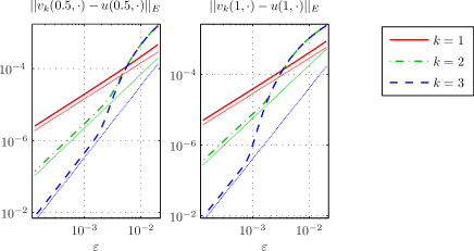
Figure 1: Single Gaussian beams: Asymptotic behavior of $v_{k}-u$ in the rescaled energy norm at $t=\{0.5,1\}$ for $k=\{1,2,3\}$ order beams. The results are shown on log-log plots along with $c_{1}\varepsilon^{1}$, $c_{2}\varepsilon^{3/2}$, and $c_{3}\varepsilon^{2}$ to help with the interpretation of the asymptotic behavior. The asymptotic behavior agrees with the analytical estimates: $1$-st order beam is $\mathcal{O}(\varepsilon^{1})$, $2$-nd order beam is $\mathcal{O}(\varepsilon^{3/2})$, and $3$-rd order beam is $\mathcal{O}(\varepsilon^{2})$.

5.2 Cusp Caustic

We consider an example in $2$D that develops a cusp caustic. The initial data for $u$ at $t=0$ is given by

$$u(0,y) =e^{-10|y|^{2}}e^{i(-y_{1}+y_{2}^{2})/\varepsilon}\ .$$

Thus, the initial phase and amplitudes are given by

$$\Phi(y)=-y_{1}+y_{2}^{2}\ ,\qquad A_{0,0}(y)=e^{-10|y|^{2}},\qquad A_{0,1}(y)=0\ .$$

For the initial data for $u_{t}(0,y)$, we take

$$u_{t}(0,y) =\left(\frac{i}{\varepsilon}\Phi_{t}(y)\left[A_{0,0}(y)+\varepsilon A_{0,1}(y)\right]+\left[A_{0,0,t}(y)+\varepsilon A_{0,1,t}(y)\right]\right)e^{i\Phi(y)/\varepsilon}\ ,$$

where the $\Phi_{t}$, $A_{0,0,t}$ and $A_{0,1,t}$ are obtained from the Gaussian beam ODEs and various $y$ derivatives of $\Phi$, $A_{0,0}$ and $A_{0,1}$. Specifically, we take $\Phi_{t}(y)=+|\nabla_{y}\Phi(y)|$ so that waves propagate in the positive $y_{1}$ direction. As was shown in [34], this particular example develops a cusp caustic at $t=0.5$ and two fold caustics for $t>0.5$.

To form the Gaussian beam superposition solutions, it is enough to consider Gaussian beams governed by $H=-|p|$, because of the initial data choice. We take the initial Taylor coefficients to be

$$x(0;z) =\begin{bmatrix}z_{1}\\ z_{2}\end{bmatrix}\ , p(0;z) =\begin{bmatrix}-1\\ 2z_{2}\end{bmatrix}\ ,$$

$$\phi_{0}(0;z) =-z_{1}+z_{2}^{2}\ , M(0;z) =\begin{bmatrix}i&0\\ 0&2+i\end{bmatrix}\ ,$$

$$\phi_{\beta}(0;z) =0,\ |\beta|=3,4\ , a_{0,\beta}(0;z) =\partial_{y}^{\beta}A_{0}(z),\ |\beta|=0,1,2\ ,$$

$$a_{1,0} =0\ ,$$

where only the necessary parameters are used for each of the $1$-st, $2$-nd and $3$-rd order beams. For $2$-nd and $3$-rd order beams, we additionally use a cutoff function with $\eta=1/10$. We propagate the Gaussian beam solutions to $t=\{0,0.25,0.5,0.75,1\}$. At each $t$, we compute the rescaled energy norm of the difference $u_{k}-u$. The asymptotic convergence as $\varepsilon\to 0$ is shown in Figure 2.

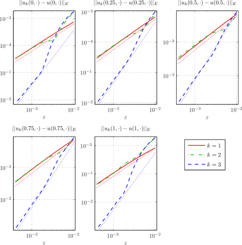
Figure 2: Superpositions of Gaussian beams for cusp caustic: Asymptotic behavior of ${u_{k}-u}$ in the rescaled energy norm at $t=\{0,0.25,0.5,0.75,1\}$ for $k=\{1,2,3\}$ order Gaussian beam superpositions. The results are shown on log-log plots along with $c_{1}\varepsilon^{1}$ and $c_{2}\varepsilon^{2}$ to help with the interpretation of the asymptotic behavior.

We draw the attention of the reader to the following features in the plots:

1. At all $t$:

   1. The asymptotic behavior of $1$-st and $2$-nd order solutions is the same and of order $\mathcal{O}(\varepsilon^{1})$.

   2. The asymptotic behavior of $3$-rd order solution is of order $\mathcal{O}(\varepsilon^{2})$.

   3. For large value of $\varepsilon$ the error for $2$-nd and $3$-rd order solutions is dominated by the error induced by the cutoff function. In this region the error decays exponentially.

   4. For midrange values of $\varepsilon$, $2$-nd order solutions experience a fortuitous error cancellation. This is due to the cutoff function. Changing the cutoff radius $\eta$ shifts this region.

2. At $t=0.5$ and $t>0.5$, the asymptotic behavior of the error is unaffected by the cusp and fold caustics, respectively.

For this example we note that the convergence rate for odd beams $k\in\{1,3\}$ is in fact half an order better than our theoretical estimates. This improvement was also observed and proved for a simplified setting in [27], where the analysis shows that the gain is due to error cancellations between adjacent beams; it is therefore not present for single Gaussian beams. The result in [27] is for the Helmholtz equation and only concerns the pointwise error away from caustics. Here the numerical results indicate that the same improvement appears for the wave equation in the energy norm even when caustics are present. We conjecture that this gain of convergence is due to error cancellations as well and that it is present for all Gaussian beam superpositions with beams of odd order $k$. Moreover, we conjecture that the theoretical result is sharp for beams of even order $k$, giving us an optimal error estimate in the energy norm of $\mathcal{O}(\varepsilon^{\lceil k/2\rceil})$ for all $k$.

6 Concluding Remarks

Gaussian beams are asymptotically valid high frequency solutions to strictly hyperbolic PDEs concentrated on a single curve through the physical domain. They can also be constructed for the Schrödinger equation. Superpositions of Gaussian beams provide a powerful tool to generate more general high frequency solutions. In this work, we establish error estimates of the Gaussian beam superposition for all strictly hyperbolic PDEs and the Schrödinger equation. Our study gives the surprising conclusion that even if the superposition is done over physical space, the error is still independent of the number of dimension and of the presence of caustics. Thus, we improve upon earlier results by Liu and Ralston [22, 23].

References

- [1] G. Ariel, B. Engquist, N. M. Tanushev, and R. Tsai. Gaussian beam decomposition of high frequency wave fields using expectation-maximization. J. Comput. Phys., 230(6):2303–2321, 2011.
- [2] V. M. Babič and V. S. Buldyrev. Short-Wavelength Diffraction Theory: Asymptotic Methods, volume 4 of Springer Series on Wave Phenomena. Springer-Verlag, 1991.
- [3] V. M. Babič and T. F. Pankratova. On discontinuities of Green’s function of the wave equation with variable coefficient. Problemy Matem. Fiziki, 6, 1973. Leningrad University, Saint-Petersburg.
- [4] V. M. Babič and M. M. Popov. Gaussian summation method (review). Izv. Vyssh. Uchebn. Zaved. Radiofiz., 32(12):1447–1466, 1989.
- [5] S. Bougacha, J.L. Akian, and R. Alexandre. Gaussian beams summation for the wave equation in a convex domain. Commun. Math. Sci., 7(4):973–1008, 2009.
- [6] V. Červený, M. M. Popov, and I. Pšenčík. Computation of wave fields in inhomogeneous media — Gaussian beam approach. Geophys. J. R. Astr. Soc., 70:109–128, 1982.
- [7] B. Engquist and O. Runborg. Computational high frequency wave propagation. Acta Numerica, 12:181–266, 2003.
- [8] N. R. Hill. Gaussian beam migration. Geophysics, 55(11):1416–1428, 1990.
- [9] N. R. Hill. Prestack Gaussian beam depth migration. Geophysics, 66(4):1240–1250, 2001.
- [10] L. Hörmander. Fourier integral operators. I. Acta Math., 127(1-2):79–183, 1971.
- [11] L. Hörmander. On the existence and the regularity of solutions of linear pseudo-differential equations. L’Enseignement Mathématique, XVII:99–163, 1971.
- [12] L. Hörmander. The analysis of linear partial differential operators. I. Classics in Mathematics. Springer, Berlin, 2003. Distribution theory and Fourier analysis, Reprint of the 1990 edition.
- [13] L. Hörmander. The analysis of linear partial differential operators. III. Classics in Mathematics. Springer, Berlin, 2007. Pseudo-differential operators, Reprint of the 1994 edition.
- [14] S. Jin, H. Wu, and X. Yang. Gaussian beam methods for the Schrödinger equation in the semi-classical regime: Lagrangian and Eulerian formulations. Commun. Math. Sci., 6:995–1020, 2008.
- [15] A. P. Katchalov and M. M. Popov. Application of the method of summation of Gaussian beams for calculation of high-frequency wave fields. Sov. Phys. Dokl., 26:604–606, 1981.
- [16] J. B. Keller. Corrected Bohr-Sommerfeld quantum conditions for nonseparable systems. Ann. Physics, 4:180–188, 1958.
- [17] L. Klimeš. Expansion of a high-frequency time-harmonic wavefield given on an initial surface into Gaussian beams. Geophys. J. R. astr. Soc., 79:105–118, 1984.
- [18] L. Klimeš. Discretization error for the superposition of Gaussian beams. Geophys. J. R. Astr. Soc., 86:531–551, 1986.
- [19] Yu. A. Kravtsov. On a modification of the geometrical optics method. Izv. VUZ Radiofiz., 7(4):664–673, 1964.
- [20] S. Leung and J. Qian. Eulerian Gaussian beams for Schrödinger equations in the semi-classical regime. J. Comput. Phys., 228:2951–2977, 2009.
- [21] S. Leung, J. Qian, and R. Burridge. Eulerian Gaussian beams for high frequency wave propagation. Geophysics, 72:SM61–SM76, 2007.
- [22] H. Liu and J. Ralston. Recovery of high frequency wave fields for the acoustic wave equation. Multiscale Model. Sim., 8(2):428–444, 2009.
- [23] H. Liu and J. Ralston. Recovery of high frequency wave fields from phase space–based measurements. Multiscale Model. Sim., 8(2):622–644, 2010.
- [24] D. Ludwig. Uniform asymptotic expansions at a caustic. Comm. Pure Appl. Math., 19:215–250, 1966.
- [25] V. P. Maslov and M. V. Fedoriuk. Semiclassical approximation in quantum mechanics, volume 7 of Mathematical Physics and Applied Mathematics. D. Reidel Publishing Co., Dordrecht, 1981. Translated from the Russian by J. Niederle and J. Tolar, Contemporary Mathematics, 5.
- [26] M. Motamed and O. Runborg. A wave front Gaussian beam method for high-frequency wave propagation. In Proceedings of WAVES 2007, University of Reading, UK, 2007.
- [27] M. Motamed and O. Runborg. Taylor expansion and discretization errors in Gaussian beam superposition. Wave Motion, 2010.
- [28] M. M. Popov. A new method of computation of wave fields using Gaussian beams. Wave Motion, 4:85–97, 1982.
- [29] J. Qian and L. Ying. Fast Gaussian wavepacket transforms and Gaussian beams for the Schrödinger equation. Journal of Computational Physics, In Press, Corrected Proof:–, 2010.
- [30] J. Ralston. Gaussian beams and the propagation of singularities. In Studies in partial differential equations, volume 23 of MAA Stud. Math., pages 206–248. Math. Assoc. America, Washington, DC, 1982.
- [31] V. Rousse and T. Swart. Global -boundedness theorems for semiclassical Fourier integral operators with complex phase. arxiv:0710.4200v3, 2007.
- [32] V. Rousse and T. Swart. A mathematical justification for the Herman–Kluk propagator. Comm. Math. Phys., 286(2):725–750, 2009.
- [33] O. Runborg. Mathematical models and numerical methods for high frequency waves. Commun. Comput. Phys., 2:827–880, 2007.
- [34] N. M. Tanushev. Superpositions and higher order Gaussian beams. Commun. Math. Sci., 6(2):449–475, 2008.
- [35] N. M. Tanushev, B. Engquist, and R. Tsai. Gaussian beam decomposition of high frequency wave fields. J. Comput. Phys., 228(23):8856–8871, 2009.
- [36] N. M. Tanushev, J. Qian, and J. V. Ralston. Mountain waves and Gaussian beams. Multiscale Model. Simul., 6(2):688–709, 2007.