On the localization of fermions in double thick $D$-branes

Abstract

Hints on the possible localization of fermions on double thick $D$-branes (Domain Walls) are found by analyzing the moduli space of parameters. Deeper analysis toward this direction might help to select phenomenologically plausible models. A new kind of condition for fermion localization is proposed. This might be useful in multi-brane-world scenarios, which are important when symmetry breaking is considered in the AdS/CFT formalism, as well as in curved brane-worlds.

I Introduction

In the last decade, after the work of Randall and SundrumRS1 ; RS2 , the study of brane-worlds have increased considerably, due to its application in explaining fundamentals problems in both particle physics and gravity.

Besides the early works Akama:1982jy ; RS ; Visser:1985qm , the importance of brane-worlds became apparent almost 20-years later, when the hierarchy problem was considered in this context RS1 , and the same authors realized that a new kind of compactification was possible RS2 , different to that proposed by Kaluza and Klein Kaluza ; Klein and its generalizations PopeKK .

On the other hand, branes are the fundamental brick for the AdS/CFT correspondence, proposed by MaldacenaMaldacena1 (see also Maldacena2 ), which allows to relate the spectrum of a string theory in a AdS background with the one of a conformal field theory at the boundary of the AdS spacetime. Throughout this article only the brane-world aspect will be considered.

Several generalizations of the Randall-Sundrum brane worlds have been considered, such as multi-brane worldsKogan:2000xc , thick branes or domain wallsGremm:1999pj , more complicated domain walls solutions with or without a well defined brane-limitMPS ; Guerrero:2005aw ; Guerrero:2005xx (for an illustration on the brane limit see GMP ), localization of gravity in different brane-world backgroundsCastilloFelisola:2004eg , localization of fermionsKehagias:2000au ; MPT and their spectrumLiu:2009dw , localization of gauge fieldsGuerrero:2009ac and many others.

The aim of this paper is to restrict the moduli space to specific variety of domain walls, known in the literature as static double walls , found in MPS and generalized in Guerrero:2005aw ; Guerrero:2005xx . Despite the existence of these generalizations, we concentrate ourselves on the original solutions. The motivation for studying these static domain walls is that they are the minimal parametric generalization of the thick version of Randall-Sundrum brane-world Gremm:1999pj , which are suitable phenomenological candidates for allowing fermion localization.

In the following section a detailed analysis of the localization of fermions is done, for static solutions. Although the procedure is known and reviewed in several articles, new considerations are made and special cases considered. In section III the analysis of the spectrum and moduli space is done for a family of static double domain walls. At the end an appendix is included to summarize notation and conventions.

II Fermion Localization on Static $D$-branes

In the following, thick-branes (or gravitational domain walls) are considered. The formal relation between the two might be established through a limit GMP .

This Domain Walls are generated by a scalar field, $\phi(\xi)$, which depends on the extra dimension, $\xi$ (see Vilenkin-book ). The spacetime has a metric whose line element is given by ,

$$ds^{2}(g)=e^{2A(\xi)}\left(-dt^{2}+e^{2B(\xi,t)}d\vec{x}^{2}\right)+e^{2C(\xi)}d\xi^{2}.$$ (1)

Several Domain Wall solutions are listed on MPS ; Guerrero:2005aw ; Guerrero:2005xx .

The 5-dimensional action for a massive fermion on a curved spacetime is given by,

$$S_{D}=\int d^{4}xd\xi\sqrt{|g|}\bar{\Psi}\left(-\not\!\nabla-M\right)\Psi,$$ (2)

where $\Psi$ is the 5-dimensional fermion, the bar indicates Dirac conjugation, $\nabla$ is the covariant derivative on the curved spacetime, $M$ is the 5-dimensional mass of $\Psi$ and $|g|$ is the absolute value of the metric determinant. The use of tetrad formalism is implicit, although the notation does not suggest it.

However, it is not possible to localize fermions on this set up Bajc:1999mh . A bypass to the problem consist in adding an interaction. A Yukawa-like interaction between the fermion an the scalar field which generates the domain wall does the work. Henceforth, the action to consider is,

$$S=S_{D}+S_{Y}=\int d^{4}x\;d\xi\sqrt{|g|}\;\bar{\Psi}\left(-\mathchoice{\mathrel{\hbox to0.0pt{\kern 4.16667pt\kern-5.27776pt$\displaystyle\not$\hss}{\nabla}}}{\mathrel{\hbox to0.0pt{\kern 4.16667pt\kern-5.27776pt$\textstyle\not$\hss}{\nabla}}}{\mathrel{\hbox to0.0pt{\kern 2.91667pt\kern-4.11108pt$\scriptstyle\not$\hss}{\nabla}}}{\mathrel{\hbox to0.0pt{\kern 2.08333pt\kern-3.3333pt$\scriptscriptstyle\not$\hss}{\nabla}}}-M+\lambda\mathcal{P}(\phi)\right)\Psi,$$ (3)

with $\mathcal{P}$ is, in general, a polynomial function on $\phi$. The simplest model is $\mathcal{P}(\phi)=\phi$, and it was considered in Bajc:1999mh with a different kind of Domain Wall than those presented here.

In the literature, it has become customary to take into account just the case when the 5-dimensional mass of the fermion vanishes, i.e. $M=0$. However, as will be discussed, $M$ could be a rather important parameter for selecting plausible phenomenological models. Therefore, the distinction between massive and massless fermions is made.

II.1 Massless 5D Fermions

In the following section a presentation of the different possible conditions which could be imposed on the fermions are given, as well as the equations of motion of their profiles .

The static Domain Wall solution given in MPS has a $B(\xi)\propto\xi$, which vanishes at the wall position. This favors to impose the ‘flat’ condition on 4-dimensional fermions, as explained on sections II.1.1 and II.1.2 below. However, in multi-brane scenarios RS1 or in curved branes Papadopoulos:1999tw , a different 4-dimensional condition could be imposed, as mentioned in sections II.1.3 and II.1.4 below.

From now on, the 5-dimensional spinor is decomposed into,

$$\Psi(x,\xi)=\psi_{+}(x)f_{+}(\xi)+\psi_{-}(x)f_{-}(\xi),$$ (4)

with $\psi_{\pm}=P_{\pm}\psi$ the 4-dimensional chiral spinors and $f_{\pm}$ their profile through the extra dimension.

II.1.1 Flat Massless 4D Fermions

For a flat brane world volume, the Dirac equations for 4D chiral massless fermions, $\psi_{\pm}$, are

$$\not\!\partial^{(4)}\psi_{\pm}=0.$$ (5)

Following the procedure described in Kehagias:2000au ; MPT , one gets the equations of motion for the profiles,

$$f^{\prime}_{\pm}+A^{\prime}f_{\pm}\mp\lambda\mathcal{P}(\phi)e^{C}f_{\pm}=0,$$ (6)

where $f_{\pm}$ are the profiles for $\psi_{\pm}$. Their solutions are,

$$f_{\pm}\propto e^{-A\pm\lambda\int d\xi\;\mathcal{P}(\phi)e^{C}}.$$ (7)

II.1.2 Flat Massive 4D Fermions

If the world volume of the brane is flat, but the 4-dimensional fermions are massive, the Dirac equation for these are,

$$\not\!\partial^{(4)}\psi_{\pm}=-m\psi_{\mp},$$ (8)

with $m$ the 4-dimensional mass. A similar procedure to the one above, yields the profile equations (see MPT ),

$$f^{\prime}_{\pm}+A^{\prime}f_{\pm}\mp\lambda\mathcal{P}(\phi)e^{C}f_{\pm}=\pm me^{-A+C}f_{\mp},$$ (9)

since massive fermions mix chiralities, the equations are coupled.

The best way of work them out is changing the variable from $\xi\to\xi^{\prime}$ where $\xi^{\prime}=\int d\xi e^{-A+C}$. Then, in terms of the new variable one gets

$$f^{\prime}_{\pm}+A^{\prime}f_{\pm}\mp\lambda\mathcal{P}(\phi)e^{A}f_{\pm}=\pm mf_{\mp},$$ (10)

with prime denoting derivative with respect to $\xi^{\prime}$.

When the equations are decoupled, a Schrödinger-like equation governs the profiles ,

$$\left[-\partial^{2}_{\xi^{\prime}}+V^{\pm}_{qm}\right]u_{\pm}=m^{2}u_{\pm},$$ (11)

where

$$f_{\pm}\mapsto e^{-2A}u_{\pm},$$

and

$$V^{\pm}_{qm}=\left(\lambda\mathcal{P}(\phi)e^{A}\right)^{2}\pm\partial_{\xi^{\prime}}\left(\lambda\mathcal{P}(\phi)e^{A}\right).$$ (12)

II.1.3 Covariantly Massless 4D Fermions

There exist branes which are not flat submanifolds embedded on the spacetime Papadopoulos:1999tw . For these general cases, the Dirac equation for 4-dimensional massless chiral fermions is given by

$$\not\!\nabla^{(4)}\psi_{\pm}=0,$$ (13)

and the profile equations are,

$$f^{\prime}_{\pm}+\frac{1}{4}\left(4A^{\prime}+{3}B^{\prime}\right)f_{\pm}\mp\lambda\mathcal{P}(\phi)e^{C}f_{\pm}=0,$$ (14)

whose solutions are,

$$f_{\pm}\propto e^{-\frac{1}{4}\left(4A+3B\right)\pm\lambda\int d\xi\;\mathcal{P}(\phi)e^{C}}.$$ (15)

II.1.4 Covariantly Massive 4D Fermions

On these curved branes, 4-dimensional massive fermions might be considered. Their Dirac equations are,

$$\not\!\nabla^{(4)}\psi_{\pm}=-m\psi_{\mp},$$ (16)

whilst the profile equations are,

$$f^{\prime}_{\pm}+\frac{1}{4}\left(4A^{\prime}+{3}B^{\prime}\right)f_{\pm}\mp\lambda\mathcal{P}(\phi)e^{C}f_{\pm}=\pm me^{C}f_{\mp}.$$ (17)

Proceeding as before, but with the changes $\xi^{\prime}=\int d\xi e^{C}$ and $f_{\pm}\mapsto e^{-\frac{4A+3B}{2}}u_{\pm}$, the Schrödinger-like equation governing the profiles is,

$$\left[-\partial^{2}_{\xi^{\prime}}+V^{\pm}_{qm}\right]u_{\pm}=m^{2}u_{\pm},$$ (18)

with

$$V^{\pm}_{qm}=\left(\lambda\mathcal{P}(\phi)\right)^{2}\pm\partial_{\xi^{\prime}}\left(\lambda\mathcal{P}(\phi)\right).$$ (19)

Remark.

Equation (19) has the same structure as (12), but the lack of the exponential functions make it looks simpler. However, non-flat domain-wall solutions are much more complicated than flat ones.

II.2 Massive 5D Fermions

Although in theories with extra dimensions it is preferred to begin with massless fermions, there exists no fundamental reason for doing so. Thus, in case 5-dimensional massive fermions are considered, the above solutions are valid after the substitution $\lambda\mathcal{P}(\phi)\to\lambda\mathcal{P}(\phi)-M$, where $M$ in the 5-dimensional mass.

From (7) and (15), it is clear that after the substitution $\lambda\mathcal{P}(\phi)\to\lambda\mathcal{P}(\phi)-M$, the localization of the positive profile, $f_{+}$, is favored in detriment of the negative one, $f_{-}$. It is possible that a critical region exists where both chiralities might be localized.

In the case of 4-dimensional massive fermions, the effect enters through the quantum mechanical potential, (12) and (19), which is a case less intuitive to analyze. However, these equations might be solved numerically. From their solutions one can argue whether or not the model is phenomenologically relevant. This analysis in done for the double domain walls in the next section.

III Double Domain Wall

In the special case of the so called double walls MPS , whose metric has a line element given by

$$ds^{2}(g)=e^{2A(\xi)}\left(\eta_{\mu\nu}dx^{\mu}dx^{\nu}+d\xi^{2}\right),$$ (20)

with a warp factor,

$$A(\xi)=-\frac{1}{2s}\ln\left(1+(\alpha\xi)^{2s}\right),$$ (21)

the scalar field is,

$$\phi(\xi)=\frac{\sqrt{6s-3}}{s}\arctan\left(\alpha\xi\right)^{s}.$$ (22)

The quantum mechanical potentials, for 5-dimensional massless fermions, and several choices of the polynomial $\mathcal{P}(\phi)$, are shown in figures 1, 3 and 4. In what follows, the parameter $\alpha$ has been set to one and the solid(dashed) line indicates the quantum mechanical potential for negative(positive) chiralities, as function of the extra coordinate $\xi$.

III.1 Massless 5-Dimensional Fermions

Following the asymptotic behavior of the profiles,

$$f_{\pm}\sim e^{\int d\xi\;\Xi(\xi)},$$ (23)

as proposed in MPT , it follows that,

$$\lambda>2\alpha\left(\frac{2s}{\pi\sqrt{6s-3}}\right)^{l},$$ (24)

with $l$ the minimum (maximum) power of the polynomial $\mathcal{P}(\phi)$ if $s\leq 13$ ($s\geq 15$).

For the plots presented above, $\lambda$ is set to

$$\lambda=3\alpha\left(\frac{2s}{\pi\sqrt{6s-3}}\right)^{m},$$ (25)

unless it is specified otherwise.

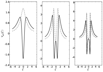
Figure 1: Quantum Mechanical potential of profiles on a DDW for linear scalar-fermion coupling. For $s\in\{1,3,5\}$

For linear scalar-fermion coupling, from figure 1 it is clear that the positive chirality fermion cannot be localized for $s=1$. However, for higher values of the coupling constant , a local well-potential appears around $\xi=0$ (see figure 2). The well gets steeper as the Yukawa coupling increases.

Figure 2: Quantum Mechanical potential of positive chirality profile on a Double DW for linear scalar-fermion coupling, $s$=1 and $\lambda$ = 1 (solid-), 2 (dashed-) and 3 (dot-dashed line).

A very interesting consequence of this is that the $\sim 10^{6}$ factor of the ratio between the Yukawa couplings of electron and neutrino could explain why right-handed neutrinos are not seen, while right-handed electrons are. The argument is as follows. The mass difference between electrons and neutrinos, explained by the Higgs mechanism, is due to the difference of their Yukawa couplings. Assume that right-handed fermions have the same mass as their left-handed partner. Independently of the Yukawa coupling, left handed fermions are localized because of the well potential $V^{-}_{qm}(\xi)$. However, $V^{+}_{qm}(\xi)$ for small Yukawa coupling (neutrino case) is a barrier potential which does not allow localization, whilst for large values of the Yukawa coupling (electron case), the appearance of a local minimum around the brane position favors the localization.

For quadratic scalar-fermion coupling, the quantum mechanical potential is not $\mathbb{Z}_{2}$-symmetric, so it is not physically relevant because the initial problem is clearly symmetric under the exchange $\xi\to-\xi$. The same argument can be applied to any even power of the scalar-fermion coupling, so they can be excluded from the analysis.

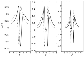
Figure 3: Quantum Mechanical potential of profiles on a DDW for quadratic scalar-fermion coupling. For $s\in\{1,3,5\}$

The analysis of the ‘spectrum’ for generalized odd scalar-fermion coupling is quite similar to the linear one, except that the “hill” potential, which forbids the localization of fermions for $\lambda<\lambda_{c}$, is not present.

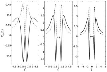
Figure 4: Quantum Mechanical potential of profiles on a DDW for cubic scalar-fermion coupling. For $s\in\{1,3,5\}$

A more detailed analysis of the spectrum of massless fermions in these family of domain wall was presented recently in Liu:2009dw .

III.2 Massive 5-Dimensional Fermions

On this section a numerical analysis of the moduli space is done. Such analysis allows to determine, point-by-point on the moduli, whether a tachyon state exists. Existence of tachyonic states turns into a phenomenological instability of the theory, which permits to rules out such a region of the moduli space, as part of a physical model.

The numerical analysis is done for the action (3), with $\lambda\geq 1.44$, which assures well-behaved asymptotic limits for left-handed fermions, as determined in MPT . Both chiralities are analyzed independently.

For solving the profile equations, a Numerov algorithm was implemented in Python and Sage sage . It proceeded as follows. First, a lattice was constructed in the moduli space. The considered lattice covers $\lambda\in[1.45,5.00]$ in steps of $0.05$, and $M\in[0.00,1.00]$ in steps of $0.02$. Secondly, the program finds $V^{\pm}_{qm}(\xi^{\prime}=0)$, and from those reference start eigen-values (which represents the 4-dimensional mass square), solves the Schrödinger-like equation for the respective “chiral” profile. Then, the value of the 4-dimensional mass square is swept by incrementing it in $0.2$ units, until a range of $\Delta m^{2}\sim 0.2$ is found, where the ground state mass eigen-value lies. Next, the bisection algorithm is applied for improving the precision of the 4-dimensional mass-square value. Finally, when the 4-dimensional mass-square for the ground state is found with an enhanced precision, one might conclude whether it is a tachyonic state, at that point in the moduli.

Table 1: Resume of the moduli space analysis.

$t$	$s$	$f^{-}$	$f^{+}$
$1$	$1$	$1.44<\lambda<3.14$	$----$
	$3$	$1.44<\lambda<3.44$	$1.44<\lambda$
	$5$	$1.44<\lambda<3.94$	$1.44<\lambda$
$3$	$1$	$----$	$1.44<\lambda$
	$3$	$----$	$1.44<\lambda$
	$5$	$1.44<\lambda<1.64$	$1.44<\lambda$
$5$	$1$	$----$	$1.44<\lambda$
	$3$	$----$	$1.44<\lambda$
	$5$	$----$	$1.44<\lambda$

The scalar-fermion coupling considered below are monomial functions of $\phi$, say, $\mathcal{P}(\phi)=\phi^{t}$, with $t\in\{1,3,5\}$. Besides, the parameter of the double walls takes similar values.

III.2.1 Linear Coupling

When the scalar-fermion coupling is linear ($t=1$), the value of $\lambda$ should be less than $3.14\pm 0.5$ for any value of $M$, in order for the left-handed ground state to be physically possible. The right-handed mode does not impose any constrain on $\lambda$.

Changes in the $s$-parameter induce changes in $\lambda_{max}$, which also varies slowly with $M$. Additionally, for large $s$, $\lambda_{max}$ increases with $M$.

As was mentioned above, there exists an energy gap between the left- and right-handed ground states.

Interestingly, in the simplest case, $s=1$, there is no possibility of ruling out the tachyonic state for the right-handed chirality. This fact somehow points to a non-minimalist model for phenomenology. All other values of $s$ possess a tachyon free spectrum.

III.2.2 Cubic Coupling

In the cubic coupling case, $\mathcal{P}(\phi)=\phi^{3}$, the right-handed profiles impose no constrain on the moduli space, whilst for $s=\{1,3\}$ the tachyonic state is always present.

For $s=5$ there exists a small window in the moduli space which allows a tachyon free spectrum, given roughly by $\lambda_{max}\gtrsim 1.64$.

III.2.3 Fifth Coupling

When the fifth coupling was considered, besides the fact that the right-handed profile imposes no constrain on the moduli space, it was not possible to get a tachyonic free spectrum for the left-handed state.

III.3 Massive 5D Fermions (Revised)

In odd number of dimensions, it is well known that there is a parity anomaly Niemi:1983rq ; Redlich:1983dv . In order to avoid this anomaly, the fermion mass in odd dimensions should be multiplied by a sign function of the scalar field Grossman:1999ra . Thus, the action is,

$$S=\int\;d^{4}x\;d\xi\;\sqrt{|g|}\bar{\Psi}\left(-\mathchoice{\mathrel{\hbox to0.0pt{\kern 4.16667pt\kern-5.27776pt$\displaystyle\not$\hss}{\nabla}}}{\mathrel{\hbox to0.0pt{\kern 4.16667pt\kern-5.27776pt$\textstyle\not$\hss}{\nabla}}}{\mathrel{\hbox to0.0pt{\kern 2.91667pt\kern-4.11108pt$\scriptstyle\not$\hss}{\nabla}}}{\mathrel{\hbox to0.0pt{\kern 2.08333pt\kern-3.3333pt$\scriptscriptstyle\not$\hss}{\nabla}}}-Msgn(\phi)+\lambda\mathcal{P}(\phi)\right)\Psi=0.$$ (26)

A numerical analysis similar to the one in the preceding subsection is done, but considering the action (26) instead of (3).

III.3.1 Negative Chiralities

For negative chiralities profiles, once more, the case with $t=s=1$ has a different behavior than the others. Tachyonic states were found all over the moduli space, except for $M=0$ and any value of $\lambda$, or for $M=0.02$ if $\lambda\geq 4.65$.

Any other choice of the parameters $M$ and $\lambda$ gives tachyon-free models. It is worth mentioning that choices $(t,s)\in\{(1,3),(1,5),(3,1)\}$ show ground states with $m^{2}$ close to zero ($m^{2}\sim 10^{-6}-10^{-8}$), although this value is far from the numerical error ($\Delta m^{2}\sim 10^{-14}$).

Due to what seems to be numerical problems in the precision, the calculations with $t=5$ could not be done.

III.3.2 Positive Chiralities

On the other hand, positive chirality profiles present no tachyonic states, at least for the considered values of $s$, $t$, $M$ nor $\lambda$. Thus, the ground state has $m^{2}>0$, but its localization is meta-stable. Besides the fact that meta-stable states rise, the question of whether these are long-lived enough, has been left aside because the main line of this work rests on formal rather than phenomenological aspects of the theory .

IV Discussion and Conclusion

First of all, a new kind of condition on the 4-dimensional fermions was considered,

$$\mathchoice{\mathrel{\hbox to0.0pt{\kern 4.16667pt\kern-5.27776pt$\displaystyle\not$\hss}{\nabla}}}{\mathrel{\hbox to0.0pt{\kern 4.16667pt\kern-5.27776pt$\textstyle\not$\hss}{\nabla}}}{\mathrel{\hbox to0.0pt{\kern 2.91667pt\kern-4.11108pt$\scriptstyle\not$\hss}{\nabla}}}{\mathrel{\hbox to0.0pt{\kern 2.08333pt\kern-3.3333pt$\scriptscriptstyle\not$\hss}{\nabla}}}\psi_{\pm}=0,$$ (27)

for finding the equations for the localized profiles, $f_{\pm}(\xi)$. Although only the conditions for localizing modes were given, this might be important when multi-brane worlds are considered, as well as non-flat branes.

The developing of a relationship between the AdS/CFT correspondence and brane-worlds (see Soda:2010si and references there in) could add importance to this particular sort of conditions, since the correspondence applies for a stack of $N$ $D$-branes. Moreover, in this scenario, the symmetry breaking might be interpreted geometrically as parallel branes slightly separated in the extra-dimension. This last set-up is exactly one kind of scenario where the new conditions might be important.

Generalizations of the profile equations were found, by allowing the scalar-fermion coupling to be non-linear, say a polynomial $\mathcal{P}(\phi)\bar{\Psi}\Psi$. When $\mathcal{P}(\phi)$ is a monomial, the physically relevant powers are odd , because for even powers on $\phi$ the quantum mechanical potential is not symmetric around the hyperplane $\xi=0$.

Polynomial couplings get complicated as soon as binomials are considered, due to the scalar coefficients which regulate the form of the quantum mechanical potential. Focused on the double domain wall family, where $s\in 2\mathbb{Z}+1$ labels the members, the condition for localizing one of the chiralities is

$$\lambda>2\alpha\left(\frac{2s}{\pi\sqrt{6s-3}}\right)^{l}.$$ (28)

with $l$ the minimum (maximum) power of the polynomial $\mathcal{P}(\phi)$ if $s\leq 13$ ($s\geq 15$).

When binomial scalar-fermion coupling are considered,

$$\mathcal{P}(\phi)=c_{1}\phi^{t_{<}}+c_{2}\phi^{t_{>}},$$ (29)

it is straightforward to note that both $t_{<}$ and $t_{>}$ should be even if the symmetric single brane scenario is examined. However, there is a chance that odd powers of $\phi$ could be phenomenologically relevant for asymmetric or multi-brane solutions.

Some constraints have been obtain for localizing both chiralities of 4-dimensional fermions coming from massive or massless 5-dimensional ones. It was found that the simplest model, $s=t=1$, does not accept localization of right chiralities, if the action (3) is consider. However, when analyzing the action (26), both chiralities could possibly be localized, and it would provide a natural explanation of the difference between the left- and right-handed neutrino mass, in those models beyond standard one where right-handed neutrinos are likely to exist, as well as the mass difference between different families of fermions. For non-linear scalar-fermion the tachyon-less constrain is made more restrictive as the non-linearity increases.

When a 5-dimensional massive fermion is considered, a slight correlation between $M$ and $\lambda$ was found, in the studied region ($0.00<M<1.00$ and $1.45<\lambda<5.00$). The considered region might be extended, but covering a larger moduli space goes beyond the scope of this work.

One might wonder that even when no additional gauge structure is given, left- and right- handed chiralities behave differently. An important question to be answered is whether charged particles could have similar behavior for both chiralities whilst neutrals do not, because particles other than neutrinos have the same mass for both chiralities. In order to follow this line a gauge field, say Abelian one, must be taken into account. This proposal could be part of future research.

Similar analysis to the one done in this work might be done for the asymmetric $D$-branes in MPS ; Guerrero:2005aw ; Guerrero:2005xx , some advances towards this are already being done by the authors.

In Gibbons:2006ge , the behavior of fermions on (anti-)kink solutions under discrete symmetries is studied. These could be used to complete a theoretical analysis on fermion localization.

Acknowledgement

We would like to thank A. Melfo, C. Dib and N. Neill for helpful discussions and comments. O.C-F. thanks ICTP-Trieste and CECS-Valvidia for there hospitality during part of the development of this work.

This work was supported in part by DGIP-UTFSM (Chile), MECESUP₂ (Chile) under the grant FSM0605-D3008, and Fondecyt project 11000287.

Appendix A Conventions and Notations

Through the manuscript, the metrics have signature mostly positive. Since the tetrads formalism is used extensively, distinction between flat and curved coordinates is made by Latin and Greek indices. Moreover, hated indices run over the whole spacetime whilst unhated ones run over a hypersurface restriction, i.e., on the coordinates parallel to the topological defect.

The gamma matrices are defined in the tangent space, and they satisfy the Clifford algebra,

$$\left\{\gamma^{\hat{a}},\gamma^{\hat{b}}\right\}=2\eta^{\hat{a}\hat{b}}\mathds{1}.$$ (30)

In even dimensions one can define the chirality matrix $\gamma^{*}$, satisfying the properties

• $\left\{\gamma^{\hat{a}},\gamma^{*}\right\}=0$.

• $(\gamma^{*})^{2}=\mathds{1}$.

From this, the projector operators,

$$P_{\pm}=\frac{\mathds{1}-\gamma^{*}}{2},$$ (31)

are both non-trivial.

In any dimension one may define a set of generators of the Lorentz algebra, constructed with the elements of the Clifford algebra (30). These generators of the Lorentz algebra are,

$$\mathscr{J}^{\hat{a}\hat{b}}=-\frac{\imath}{4}\left[\gamma^{\hat{a}},\gamma^{\hat{b}}\right].$$ (32)

When the Dirac-Feynman slash notation is used it must be interpreted as,

$$\mathchoice{\mathrel{\hbox to0.0pt{\kern 2.65451pt\kern-5.27776pt$\displaystyle\not$\hss}{\partial}}}{\mathrel{\hbox to0.0pt{\kern 2.65451pt\kern-5.27776pt$\textstyle\not$\hss}{\partial}}}{\mathrel{\hbox to0.0pt{\kern 1.85815pt\kern-4.11108pt$\scriptstyle\not$\hss}{\partial}}}{\mathrel{\hbox to0.0pt{\kern 1.32726pt\kern-3.3333pt$\scriptscriptstyle\not$\hss}{\partial}}}=E^{\hat{\mu}}_{\hat{a}}\gamma^{\hat{a}}\partial_{\hat{\mu}}.$$ (33)

The covariant derivative for gauge theories is defined by,

$$\nabla_{\hat{\mu}}=\partial_{\hat{\mu}}-\imath gA_{\hat{\mu}}-\imath\Omega_{\hat{\mu}},$$ (34)

with $\Omega$ the gravitational connection, which is related to the Christoffel connection for integer spin fields, and with the spin connection for semi-integer spin fields. Clearly the Dirac-Feynman slash notation can be used with the covariant derivative,

$$\mathchoice{\mathrel{\hbox to0.0pt{\kern 4.16667pt\kern-5.27776pt$\displaystyle\not$\hss}{\nabla}}}{\mathrel{\hbox to0.0pt{\kern 4.16667pt\kern-5.27776pt$\textstyle\not$\hss}{\nabla}}}{\mathrel{\hbox to0.0pt{\kern 2.91667pt\kern-4.11108pt$\scriptstyle\not$\hss}{\nabla}}}{\mathrel{\hbox to0.0pt{\kern 2.08333pt\kern-3.3333pt$\scriptscriptstyle\not$\hss}{\nabla}}}=E^{\hat{\mu}}_{\hat{a}}\gamma^{\hat{a}}\nabla_{\hat{\mu}}=E^{\hat{\mu}}_{\hat{a}}\gamma^{\hat{a}}\left(\partial_{\hat{\mu}}-\imath gA_{\hat{\mu}}-\imath\Omega_{\hat{\mu}}\right).$$ (35)

References

- (1) Lisa Randall and Raman Sundrum. A large mass hierarchy from a small extra dimension. Phys. Rev. Lett., 83:3370–3373, 1999.
- (2) Lisa Randall and Raman Sundrum. An alternative to compactification. Phys. Rev. Lett., 83:4690–4693, 1999.
- (3) K. Akama, Lect. Notes Phys. 176 (1982) 267 [arXiv:hep-th/0001113].
- (4) V. A. Rubakov and M. E. Shaposhnikov. Do We Live Inside a Domain Wall? Phys. Lett., B125:136–138, 1983.
- (5) M. Visser, Phys. Lett. B 159, 22 (1985) [arXiv:hep-th/9910093].
- (6) Theodor Kaluza. On the Problem of Unity in Physics. Sitzungsber. Preuss. Akad. Wiss. Berlin (Math. Phys. ), 1921:966–972, 1921.
- (7) O. Klein. Quantum theory and five-dimensional theory of relativity. Z. Phys., 37:895–906, 1926.
- (8) C. N. Pope. Kaluza-klein theory. Technical report, TAMU. Lecture Notes.
- (9) Juan Martin Maldacena. The large N limit of superconformal field theories and supergravity. Adv. Theor. Math. Phys., 2:231–252, 1998.
- (10) Ofer Aharony, Steven S. Gubser, Juan Martin Maldacena, Hirosi Ooguri, and Yaron Oz. Large N field theories, string theory and gravity. Phys. Rept., 323:183–386, 2000.
- (11) Ian I. Kogan, Stavros Mouslopoulos, Antonios Papazoglou, and Graham G. Ross. Multi-brane worlds and modification of gravity at large scales. Nucl. Phys., B595:225–249, 2001.
- (12) Martin Gremm. Four-dimensional gravity on a thick domain wall. Phys. Lett., B478:434–438, 2000.
- (13) Alejandra Melfo, Nelson Pantoja, and Aureliano Skirzewski. Thick domain wall spacetimes with and without reflection symmetry. Phys. Rev., D67:105003, 2003.
- (14) Rommel Guerrero, R. Omar Rodriguez, and Rafael S. Torrealba. De Sitter and double asymmetric brane worlds. Phys. Rev., D72:124012, 2005.
- (15) Rommel Guerrero, R. Ortiz, R. Omar Rodriguez, and Rafael S. Torrealba. De Sitter and double irregular domain walls. Gen. Rel. Grav., 38:845–855, 2006.
- (16) Rommel Guerrero, Alejandra Melfo, and Nelson Pantoja. Self-gravitating domain walls and the thin-wall limit. Phys. Rev., D65:125010, 2002.
- (17) Oscar Castillo-Felisola, Alejandra Melfo, Nelson Pantoja, and Alba Ramirez. Localizing gravity on exotic thick 3-branes. Phys. Rev., D70:104029, 2004.
- (18) A. Kehagias and K. Tamvakis. Localized gravitons, gauge bosons and chiral fermions in smooth spaces generated by a bounce. Phys. Lett., B504:38–46, 2001.
- (19) Alejandra Melfo, Nelson Pantoja, and Jose David Tempo. Fermion localization on thick branes. Phys. Rev., D73:044033, 2006.
- (20) Yu-Xiao Liu, Chun-E Fu, Li Zhao, and Yi-Shi Duan. Localization and Mass Spectra of Fermions on Symmetric and Asymmetric Thick Branes. Phys. Rev., D80:065020, 2009.
- (21) Rommel Guerrero, Alejandra Melfo, Nelson Pantoja, and R. Omar Rodriguez. Gauge field localization on brane worlds. 2009.
- (22) B. Bajc and G. Gabadadze, “Localization of matter and cosmological constant on a brane in anti de Sitter space,” Phys. Lett. B 474, 282 (2000) [arXiv:hep-th/9912232].
- (23) G. Papadopoulos, J. G. Russo and A. A. Tseytlin, Class. Quant. Grav. 17, 1713 (2000) [arXiv:hep-th/9911253].
- (24) W. A. Stein et al. Sage Mathematics Software (Version 4.4.1). The Sage Development Team, 2010. http://www.sagemath.org.
- (25) Tony Gherghetta and Alex Pomarol. Bulk Fields and Supersymmetry in a Slice of AdS Nucl.Phys. B586:141-162, 2000.
- (26) A. Vilenkin and E. P. S. Shellard. Cosmic strings and other topological defects. CUP, 1994.
- (27) A. J. Niemi and G. W. Semenoff, Phys. Rev. Lett. 51, 2077 (1983).
- (28) A. N. Redlich. Parity Violation and Gauge Noninvariance of the Effective Gauge Field Action in Three-Dimensions. Phys. Rev., D29:2366–2374, 1984.
- (29) Yuval Grossman and Matthias Neubert. Neutrino masses and mixings in non-factorizable geometry. Phys. Lett., B474:361–371, 2000.
- (30) C. Ringeval, P. Peter and J. P. Uzan, Phys. Rev. D 65, 044016 (2002) [arXiv:hep-th/0109194].
- (31) G. Gibbons, K. i. Maeda and Y. i. Takamizu, Phys. Lett. B 647, 1 (2007) [arXiv:hep-th/0610286].
- (32) Jiro Soda. AdS/CFT on the brane. 2010.