Mass Functions in Fractal Clouds: The Role of Cloud Structure in the Stellar Initial Mass Function

Abstract

The possibility that the stellar initial mass function (IMF) arises mostly from cloud structure is investigated with fractal Brownian motion (fBm) clouds that have power-law power spectra. An fBm cloud with a realistic projected power spectrum slope of $\beta=2.8$ is found to have a mass function for clumps exceeding a threshold density that is a power-law with a slope of $\alpha=2.35$, the same as in the Salpeter IMF. Any hierarchically structured cloud has a clump mass function with about the same slope. This result implies that turbulent interstellar clouds produce dense substructure with the observed pre-stellar core mass function built in from the start. Details of the clump formation processes are not critical. The conversion of clumps into stars involves a second step. A one-to-one correspondence between clump mass and star mass is not necessary to convert the clump mass spectrum into an IMF with the same power-law slope. As long as clumps have an internal stellar IMF from sub-fragmentation, protostellar accretion, coalescence and other processes, and the characteristic mass for this internal IMF scales with the clump mass, then the IMF slope above the minimum characteristic mass will equal the clump mass slope. A detailed review of IMF models illustrates the prominence of cloud structure as a major component in a wide class of theories. Tests are proposed to determine the relative importance of cloud structure and competitive accretion in the IMF.

Received ______________/ Accepted _________________

1 Introduction

1.1 Clump Mass Functions and Power Spectra

Interstellar gas emission has a power-law power spectrum suggesting structure on a wide range of scales (Crovisier & Dickey, 1983; Green, 1993; Dickey, McClure-Griffiths, Stanimirović, Gaensler & Green, 2001; Miville-Desch${\hat{\rm e}}$nes, Joncas, Falgarone & Boulanger, 2003, 2003; Miville-Desch${\hat{\rm e}}$nes, Martin & et al., 2010). Cloud-fitting algorithms that are applied to this structure find power law mass functions for the emission peaks, which are usually identified as clouds, clumps, and cores (Williams, de Geus & Blitz, 1994; Stützki & Güesten, 1990). Because there is considerable interest in the origin of various interstellar and stellar mass functions, such as those for giant molecular clouds, molecular cloud clumps, star clusters, and individual stars, we would like to understand the relationship between the structure that is viewed as a featureless power spectrum and the structure that is inferred to be a collection of discrete objects.

Stützki et al. (1998) suggested that for Gaussian-shaped clouds with a mass-radius relation $M\propto R^{\gamma}$ and a power law mass function of slope $-\alpha$, the slope $-\beta$ of the power spectrum is given by $\beta=\gamma\left(3-\alpha\right)$. This relation comes from an integral over the cloud mass function, $dn\propto M^{-\alpha}dM$, of the contribution to the power spectrum, $dP(k)$, from a cloud of mass $M$, which is $dP(k)\propto M^{2}\exp(-0.5k^{2}R^{2})dn$. The result is the frequency ($k$) dependent part of the integral over $M^{2-\alpha}\exp(-0.5k^{2}R^{2})dM$, which is $k^{-\beta}$ for the above value of $\beta$. Stützki et al. (1998) noted that the value of $\beta\sim 2.8$ they observed corresponded to typical $\alpha\sim 1.6$ and $\gamma\sim 2$ for molecular clouds. Observations of $\beta$ for various regions of the Milky Way are in Table 1; generally $\beta\sim 2.8$.

Table 1: Observations of Power Spectrum Slope $\beta$ for various regions of the Milky Way.

	Region				Type of Observation				Power Spectrum Slope	Reference
									($\beta$)
	Foreground of Cas A				HI 21 cm absorption				$2.75\pm 0.25$	Deshpande et al. (2000)
	”				”				$2.86\pm 0.1$	Roy et al. (2010)
	Perseus, Taurus, Rosetta clouds				12CO				$2.74\pm 0.08$	Padoan et al. (2004)
	Perseus cloud				13CO				$2.86\pm 0.1$	Padoan et al. (2006)
	”				12CO and 13CO				$\approx 3.1$	Sun et al. (2006)
	Perseus spiral arm				HI 21 cm				$2.2$ to $3.0$	Green (1993)
	Ursa Major high-latitude cirrus				HI 21 cm				$3.6\pm 0.2$	Miville-Desch${\hat{\rm e}}$nes et al. (2003)
	Polaris Flare				12CO				$\sim 2.8$	Stützki et al. (1998)
	”				FIR				$2.7\pm 0.1$	Miville-Desch${\hat{\rm e}}$nes et al. (2010)
	Several molecular clouds				12CO and 13CO				2.5 to 2.8	Bensch et al. (2001)
	”				100 $\mu$m				2.9 to 3.2	Gautier et al. (1992)
	The Fourth Galactic Quadrant				HI 21 cm				$\sim 4$	Dickey et al. (2001)
	The Gum nebula				8, 24, and 70 $\mu$m				2.6 to 3.5	Ingalls et al. (2004)

Hennebelle & Chabrier (2008) derived the cloud mass distribution from a power spectrum in a different way. They assumed that the logarithm of the density, rather than the density, has a power-law power spectrum (following Beresnyak et al. (2005)), and they considered a log-normal density pdf, ${\cal P}(\rho,R)$, for scale $R$. Then they equated the total mass of clouds more massive than $M$ from the integral over the mass function, $\int_{M}M^{\prime}n(M^{\prime})dM^{\prime}$, to the total mass in the pdf at densities higher than $\rho=M/R^{3}$, which is $M_{\rm pdf}(\rho,R)=\int_{\rho}{\cal P}(\rho^{\prime},R)d\rho^{\prime}$. This gives $n(M)=M^{-1}dM_{\rm pdf}(\rho,R)/dM=M^{-1}(dR/dM)dM_{\rm pdf}(\rho,R)/dR$. The pdf ${\cal P}$ depends on $R$ because the dispersion $\sigma$ of the log normal function was assumed to depend on $R$, as $\sigma^{2}=\sigma_{0}^{2}\left(1-\left(R/L\right)^{n^{\prime}-3}\right)$ for $n^{\prime}>3$. That is, the density fluctuations become smaller when averaged over larger scales, up to the system scale $L$. This dependence comes from the assumption $\sigma^{2}\propto\int_{2\pi/L}^{2\pi/R}k^{-n^{\prime}}d^{3}k$ where $n^{\prime}$ is the (negative) slope of the power-law power spectrum for $\log(\rho)$. The result is that $n(M)\propto M^{-1}\sigma^{-3}(dR/dM)(d\sigma^{2}/dR)\propto M^{-2}M^{n^{\prime}/3-1}=M^{-\alpha}$ for $R<<L$, where $\alpha=3-n^{\prime}/3$. This is about the same as in Stützki et al. (1998), who had $\alpha=3-\beta/3$ for $M\propto R^{3}$, considering that $\beta$ in Stützki et al. (1998) was the power spectrum slope for density while $n^{\prime}$ in Hennebelle & Chabrier (2008) was the power spectrum slope for log-density.

The Hennebelle & Chabrier (2008) model has a different relation between $\alpha$ and $\beta$ when $n^{\prime}<3$, because then $\sigma^{2}=\sigma_{0}^{2}\left((L/R)^{3-n^{\prime}}-1\right)$ diverges as $R$ goes to zero. When $n^{\prime}>3$ as in the previous paragraph, $\sigma$ approached a constant for small $R$ and its presence as $\sigma^{-3}$ in the expression for $n(M)$ contributed no additional mass dependence; only $d\sigma^{2}/dR$ contributed, making $n(M)\propto M^{-2}Rd\sigma^{2}/dR\propto M^{-3+n^{\prime}/3}$ as above. When $n^{\prime}<3$, however, $\sigma$ contains a strong $M$ dependence and the $\sigma^{-3}$ term is important, as is the $\sigma^{2}$ in another term, $(\delta_{c}+\sigma^{2}/2)$, which comes from the log-normal density distribution for threshold density $\delta_{c}$. This makes $n(M)\propto M^{-2}\sigma^{-1}Rd\sigma^{2}/dR\propto M^{-2}\sigma\propto M^{-2.5+n^{\prime}/6}$.

1.2 Clump Mass Functions and Hierarchical Structure

For hierarchically structured objects, the mass function $n(M)$ always has a power law slope $\alpha=2$ if the total mass of clouds in a logarithmic mass interval around a particular mass is the same for all masses, i.e., for all levels in the hierarchy. Then $MdN(M)/d\log M=$ constant for mass function $N$ in $\log M$ intervals, giving $N(M)\propto M^{-1}$, or $n(M)\propto M^{-2}$ for linear $M$ intervals. This $\alpha=2$ result can be derived in many ways. Clouds with an average of $N$ substructures per structure in all levels $L$ of the hierarchy have a number of objects per logarithmic mass interval that increases as $N^{L}$ and a mass per object that decreases as $1/N^{L}$, making $dN/d\log M\propto M^{-1}$ (Fleck, 1996). Similarly, the probability of selecting out of all $\log M$ levels a particular structure with mass $M$ is proportional to the number $N$ of these objects, which is also $\propto M^{-1}$ for $\log M$ intervals. The same result applies to packing scale-free structures in a volume. For wavenumber $k$ proportional to the inverse of the size, the number of structures between $k$ and $k+dk$ that fit into a space with dimension $D$ is $\xi(k)dk\propto k^{D-1}dk$, and the mass of each is $M\propto k^{-D}$. Converting wavenumber counts into mass counts using the one-to-one correspondence, $\xi(k)dk=n(M)dM$, we derive $n(M)\propto k^{D-1}dk/dM\propto k^{2D}\propto M^{-2}$, independent of dimension $D$. The Hennebelle & Chabrier (2008) result for non-gravitating clouds is shallower than $M^{-2}$ by the index $n^{\prime}/3-1=2/9$ for $n^{\prime}=11/3$ because the total cloud mass in each $\log M$ interval is not constant with $M$, but decreases with increasing $M$ as the pdf becomes narrower and the integral of the pdf above a threshold density becomes smaller.

1.3 The Stellar Initial Mass Function

The initial mass function for stars (IMF) seems considerably more difficult to understand than the mass function for non-gravitating clouds because the IMF involves the whole star formation process, including a wide range of densities and diverse physical effects. Still, the IMF in clusters is often observed to have a power law component spanning 1.5 to 2 orders of magnitude in the range from $\sim 0.5\;M_{\odot}$ to $50\;M_{\odot}$. How much of this power law comes from a power-law in cloud structure and how much comes from other processes is not currently known. Current explanations for the IMF consider cloud fragmentation driven by supersonic turbulence and self-gravity, clump coalescence, and protostellar accretion (see reviews in Bonnell et al., 2007; Dib et al., 2010; Bastian et al., 2010).

Padoan & Nordlund (2002) considered an IMF model based on turbulent fragmentation of a cloud. They proposed that turbulence compresses the gas into layers of thickness $L\propto V_{0}^{-1}$ for ambient turbulent speed $V_{0}\propto L_{0}^{\eta}$, initial length $L_{0}$, and Kolmogorov exponent $\eta\sim 1/3$. They also assumed that the number of stars scales with $L_{0}^{-3}d\log L_{0}$ from close packing (as above, where we wrote $\xi(k)dk\propto k^{3}d\log k$ for $k=1/L_{0}$ in 3D). Then with $M\propto\rho L^{3}=\rho_{0}L_{0}L^{2}$ for cubic regions in the compressed layer and density $\rho=\rho_{0}L_{0}/L$ for uncompressed density $\rho_{0}$, it follows that $M\propto L_{0}^{3}\left(L/L_{0}\right)^{2}\propto L_{0}^{3-2\eta}$. Thus $dN(M)/d\log M\propto L_{0}^{-3}\propto M^{3/\left(2\eta-3\right)}\sim M^{-1.3}$ when $\eta=1/3$, which is close to the Salpeter IMF, $dN/d\log M\propto M^{-1.35}$. The final IMF was assumed to be this clump mass function multiplied by the probability that a clump of mass $M$ exceeds the thermal Jeans mass; the pdf for thermal Jeans masses comes from the pdf for density at a constant temperature. Their clump model steepens the mass function slope above the value of $-1$ for mass-conserving fragmentation because they limit the number of stars that can form in each layer of dimension $L\times L_{0}\times L_{0}$ to a constant, even though the available space scales with $L_{0}^{2}$, i.e., $(L_{0}/L)^{2}$ cubical volumes fit in this layer. If each of these cubes were to form a star, then $N(M)$ would be larger by the factor $(L_{0}/L)^{2}$ and we would retrieve the purely hierarchical result, $dN(M)/d\log M\propto M^{-1}$.

Padoan et al. (1997) and Hennebelle & Chabrier (2008) proposed a different model for cloud fragmentation in the self-gravitating case. They start with the expression written above for a non self-gravitating cloud, $n(M)\propto M^{-1}dM_{\rm pdf}(\rho,R)/dM$, but then consider the unstable regions with average density $\rho$ larger than the density at which the Jeans length equals $R$. Instead of summing the cloud masses above $\rho R^{3}$, they sum the cloud masses smaller than $\rho R^{3}$, because the cloud’s mass will be less than the Jeans mass at length $R$ when the density exceeds the Jeans-length density. The result is $n(M)\propto M^{-1}(d\rho/dM)P_{\rm pdf}(\rho,R)$ where $\rho$ is the density giving $M=M_{J}$. Padoan et al. (1997) assume the masses are thermal Jeans masses, in which case $M\propto\rho^{-0.5}$. Hennebelle & Chabrier (2008) consider a turbulent medium, for which $M_{J}\sim GV^{2}R\propto R^{2\eta+1}$ when $V\propto R^{\eta}$, and then $\rho\sim M_{J}/R^{3}\propto R^{2\eta-2}\propto M^{(2\eta-2)/(2\eta+1)}$. In both cases, the mass function is the product of a power law and a log-normal. In part of the mass range, the slope has the Salpeter value.

Dib et al. (2010) presented a semi-analytical model to describe the simultaneous evolution of the dense core mass function and the IMF, considering accretion and feedback by winds. The basic core mass function came from Padoan & Nordlund (2002). The results showed mass functions that varied throughout the cloud and changed with time. The final functions were those at the time when pre-stellar winds disrupted the cloud, and they compared well with the core and stellar mass functions in Orion. Because the underlying model is the core function in Padoan & Nordlund (2002), geometric effects play an important role in their IMF.

All of the analytical models just described have an $\alpha=2$ power law as an underlying mass function, modified in the various cases by more or less total mass being included in logarithmic intervals as a function of the cloud mass. The models that begin with an equation $Mn(M)=dM_{\rm pdf}(\rho,R)/dM$ for $M_{\rm pdf}$ from the density pdf effectively assume that an increment toward larger or smaller mass in the mass function corresponds to an increment in density. For the IMF models, this means that massive stars correspond to low density clouds or parts of clouds. This is contrary to the mass segregation that is often observed in young clusters, and requires accretion or coagulation as a second step. The same mass-density relation results from any isothermal model that identifies star mass with Jeans mass along the power law part of the IMF. To avoid this contradiction, the pre-stellar gas temperature has to increase with core mass (e.g., Krumholz et al., 2010).

1.4 The Press and Schechter Mass Function

The cosmological equivalent of these derivations was considered by Press & Schechter (1974). They assumed infinitesimal perturbations in an expanding universe and determined the mass function of bound objects as a function of time. The initial density was assumed to have a power spectrum, $P(k)$, and the distribution function, $\cal P$, for density perturbation amplitude $\delta$ inside a given scale $R$ was assumed to be Gaussian in $\delta$ with dispersion $\sigma$ given by $\sigma^{2}=(2\pi)^{-3}\int d^{3}kP(k)W^{2}(R,k)$. The window function $W(R,k)$ was introduced by Padmanabhan (1993) to avoid a divergence at high $k$ when $\beta<3$; a Gaussian form $W\sim\exp\left(-0.5k^{2}R^{2}\right)$ was assumed. If $\delta_{c}$ is the critical density at the initial time that makes a perturbation bound at the present time, then the fraction of bound objects at the present time with masses larger than $M$ is $F(M)=\int_{\delta_{c}}^{\infty}{\cal P}d\delta.$ The co-moving mass distribution function is then $n(M)=(\rho/M)dF/dM$. This procedure is similar to that followed by Hennebelle & Chabrier (2008), except that Hennebelle & Chabrier (2008) also have a lower limit to $k$ in the integral for $\sigma$. This lower limit introduces a constant part in the expression for $\sigma^{2}$, and causes the mass-dependence of $\sigma$ to be negligible when $n^{\prime}$ ($\beta$ in our notation) exceeds 3 in the Hennebelle & Chabrier (2008) model. Without a lower limit on $k$, the cosmological mass function is $n(M)\propto M^{-2}\sigma^{-1}\exp\left(-\delta_{c}^{2}/2\sigma^{2}\right)$, which is the Press & Schechter (1974) result. Note the purely geometric component, $M^{-2}$, as in the other mass function models discussed above. For initial power spectrum $P(k)\propto k^{-\beta}$ and mass $M\propto k^{-3}$, the dispersion in the density distribution function is $\sigma\propto M^{(\beta-3)/6}$. Then $n(M)\propto M^{-2}M^{(3-\beta)/6}\exp\left(-0.5\left[M/M_{tr}\right]^{(3-\beta)/3}\right)$. This mass function is a power law truncated by an exponential. The truncation mass, $M_{tr}$, is the mass that is at the critical density for boundedness at the present time. The slope of the power law part, $\alpha=1.5+\beta/6$, has a positive correlation between $\alpha$ and $\beta$, unlike the Stützki et al. (1998) and Hennebelle & Chabrier (2008) slopes. We return to this point again in Section 3.2.

1.5 The IMF in Numerical Simulations: Competitive Accretion or Cloud Structure?

Numerical simulations of star formation have a different approach. They explain the IMF by analogy to the mass distribution of sink particles formed in the simulation (e.g., Tilley & Pudritz, 2007; Padoan et al., 2007; Li et al., 2004; Nakamura & Li, 2005, 2007; Martel et al., 2006; Bate, 2009). There are many physical processes involved, and it is not generally clear which dominate the IMF. Moreover, the simulations differ from each other in the presence of magnetic forces, magnetic diffusion, turbulence driving, initial cloud boundedness, gas cooling, stellar outflows, starlight heating, and other properties, even though they get about the same IMF. One thing they have in common is a turbulent gas, which means hierarchical structure with an $M^{-2}$ underpinning for mass functions. But there are other things in common too.

It is instructive to see what differs in the few simulations that gave another IMF. Two produced relatively flat IMFs: one model in Klessen (2001) that had small-scale turbulence driving, and models in Clark et al. (2008) that had transient unbound clouds. What they had in common was isolated star formation in non-hierarchical clouds, as determined by a short driving scale in the first case and by rapid cloud expansion in the second. They also differed from the usual simulations in having no competition among protostars for the gas: one sink particle formed in each fragment with an overall efficiency that was low.

Competitive accretion (Zinnecker, 1982; Bonnell, Bate, Clarke & Pringle, 2001, 2001) involves cloud mass (and ultimately sink particle mass) that comes from all over a cloud, independent of the initial mass of the clump that is accreting (e.g., Clark & Bonnell, 2006; Smith et al., 2008). The final star mass then depends on the accretion rate integrated over time. This mass can be small if the star is ejected from its gas reservoir early (Reipurth & Clarke, 2001; Bate et al., 2002), or if the accretion is slowed by any of a number of processes, such as tidal forces in a cluster (Bonnell et al., 2008), low local densities, or relative motions between the protostar and the gas (Clark et al., 2009). If competitive accretion is dominant over geometric effects, then it should give the Salpeter IMF in a uniform static cloud that is artificially seeded with initially identical, moving protostars. The simulated clouds that get a normal IMF are not uniform like this. They are always hierarchically structured, or they have a hierarchy of initially converging velocities that lead to hierarchical fragmentation on the same time scale as star formation. The sink particles take gas from these fragments and from the condensing proto-fragments.

The question we ask is whether the mass function of the gas reservoirs plays an important role in the final mass function of the stars. Even though accretion is the local process by which stars assemble their mass, the amount of accreted mass could depend more on the developing cloud structure (filaments, clumps, etc.) than on the presence of near-neighbors in a competitive environment. Everywhere competitive accretion occurs, cloud fragmentation also occurs at an earlier stage. Which dominates the power law part of the IMF?

A test for the origin of the IMF in simulations might be to construct clouds with different density and velocity power spectra and to see if the resulting slope of the IMF depends on the slope of these spectra, as in the Stützki et al. (1998) derivation (also found in our models below). If it does, then cloud structure would seem to have an important role in the IMF. If it does not, and all density power spectra lead to the same IMF, then we can probably rule out cloud structural effects and clump mass functions for the simulated IMFs.

One argument that cloud structure does not play an important role was given by Clark, Klessen & Bonnell (2007). They suggested that if fragmentation continues during star formation, and if the fragmentation time is shorter for smaller scales, which is likely, then the IMF from the time-integral over all cores should be steeper than the instantaneous core mass function. The observations, however, indicate that core mass functions have the same slope as the IMF (e.g., Motte, André & Neri, 1998; Rathborne, Lada, Muench, Alves, Kainulainen & Lombardi, 2009). Considering time evolution, the IMF becomes $\propto\omega(k)k^{2}dk$, where $\omega(k)$ is the formation rate of structures with wavenumber $k$, and $k^{2}dk$ is the space-filling partition function discussed above (e.g., di Fazio, 1986). For turbulence, $\omega(k)\sim\sigma(k)k$, where $\sigma(k)$ is the turbulent speed. Setting $\sigma(k)\propto k^{-\eta}$ for Kolmogorov turbulence exponent $\eta$, we get $\omega(k)\propto k^{1-\eta}$. If $M\propto k^{-3}$ for some characteristic density at collapse, then we get a mass function for linear intervals of mass $dn(M)/dM\propto k^{3-\eta}dk/dM\propto M^{-2-\left(1-\eta\right)/3}$. This is the same as the mass function derived above for space filling structures, but now it has a slope that is steeper by $\left(1-\eta\right)/3\sim 2/9$ for $\eta=1/3$ as a result of the time dependence. Palouš (2007) used this technique to derive the mass function of fragments in an expanding shell. If the IMF power law is not steeper by at least $2/9$ compared to the clump mass power law, then the IMF would seem to have a different origin than the clumps. Dib et al. (2010) got around this problem by including accretion onto the clumps. This shifts the mass function to higher values and offsets the steepening from the time dependence.

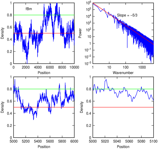
Figure 1: (Top left)Density scan of a 1D fBm cloud with two sample thresholds for clump definition. (Top right) Power spectrum of the density scan. (Lower left) Enlargement of a section of the fBm cloud, as indicated by the positions on the abscissa. (Lower right) Greater enlargement of the same cloud.

1.6 This Paper: Mass Functions in Fractal Clouds for Clumps that Exceed a Threshold Density

Here we are interested more generally in mass functions for hierarchical and fractal clouds. We determine the mass function for all clumps denser than a fixed value in a fractal cloud with a given power-law power spectrum. The dependency of the mass function on the power spectrum and density threshold are determined. The star formation process itself is not considered, nor is the IMF below the plateau at around $0.3\;M_{\odot}$. Several possible connections between our results and the full IMF are discussed in Section 4.

An approximately fixed density threshold for star formation makes sense physically Elmegreen (2007). Magnetic diffusion should suddenly become more rapid at a density of $\sim 10^{5}$ cm^-3 because the density scaling for the electron fraction becomes steeper, changing from $n^{-1/2}$ to $n^{-1}$. This steepening occurs because charge exchange replaces dissociative recombination for the neutralization of ionic molecules, and electron recombination on neutral grains replaces dissociative recombination with ionic molecules (see Fig. 1 in Elmegreen, 1979; Draine & Sutin, 1987). If the power of density exceeds $2/3$, then the time for an initially subcritical core to start collapsing is comparable to the initial free fall time (Hujeirat, Camenzind & Yorke, 2000). This is an important condition for star formation.

Dust grains and their coupling to the magnetic field also change at this density. Small grains normally dominate the viscous cross section for magnetic diffusion because of their high number density, but PAH molecules and small grains begin to disappear at densities in excess of $\sim 10^{5}$ cm^-3 (Boulanger et al., 1990). Gas depletion at high density removes ionic metals, and this also lowers the ionization fraction and promotes enhanced magnetic diffusion. The depletion time, $10^{10}/n$ years (Omont, 1986), becomes smaller than the dynamical time, $\left(G\rho\right)^{-1/2}$, when the density, $n$, exceeds $3\times 10^{4}$ cm^-3. Grain coagulation at this density becomes important too, and this reduces the number of charged grains and the net coupling of charged grains to neutrals (Flower, Pineau Des Forêts & Walmsley, 2005). Further coupling loss arises because large grains lose their field line attachment at high density (Kamaya & Nishi, 2000). All of these microscopic effects should significantly speed up gas collapse at a density near $\sim 10^{5}$ cm^-3 because they allow the magnetic field to leave the neutral gas more quickly. The mass distribution of clumps at this density should then have an imprint on the final stellar mass distribution. The final mechanisms for collapse into stars could be less important to the IMF than the mass function of clumps at the threshold density where the collapse begins.

We also study whether higher density limits produce steeper or narrower mass functions. Such an effect might explain why the power spectrum slope for the densest cores (which is like the Salpeter IMF slope of $-2.35$) is steeper than the power spectrum slope for low-density clouds (which is $\alpha\sim 1.6-1.8$). It might also explain the apparent steepening of the IMF in galactic regions that have generally low densities, as in low surface brightness spirals (Lee et al., 2004), dwarf galaxies (Hoversten & Glazebrook, 2008; Hunter et al., 2010), and the outer regions of spirals (Meurer et al., 1996; Lee et al., 2009). The IMF would get steeper in these regions if stellar mass is related to clump mass, if there is a characteristic density at which stars form, and if the clump mass function gets steeper at higher relative densities.

We previously found such a correlation between the slope of the mass function and the threshold density for clump recognition (Elmegreen, 2002; Elmegreen et al., 2006). Both studies used three-dimensional fractal Brownian motion (fBm) clouds with log-normal density pdfs. Here we experiment with fBm clouds again, first in one-dimension where the counting statistics are extremely good, and then in three dimensions, which is more relevant to star formation. Interstellar clouds are not the same as fBm clouds, but the geometric resemblance is not bad if we want to address only simple questions. For example, fractal Brownian motion clouds can be made with the same power spectrum as interstellar clouds, and they can have the same density pdf. In MHD turbulence simulations, Dib et al. (2008) also found a steepening of the mass function at higher gas density, although they commented that this steepening was the result of stronger self-gravity at higher densities. Our experiments have no self-gravity and are relevant only to the geometric aspects of cloud structure.

The dependence of the mass function slope $\alpha$ on the power spectrum slope $\beta$ is considered in detail. Generally we expect steeper power spectra to correspond to shallower mass functions. This is because steeper power spectra have relatively more structure on larger scales, which means larger masses, so the corresponding mass function has relatively more high mass clumps. Clumps are defined differently here than in Press & Schechter (1974) or Hennebelle & Chabrier (2008). Here a clump has every part of it above a threshold density and the entire matter inside the clump boundary is counted in the clump mass. In Press & Schechter and in Hennebelle & Chabrier, the average density of a clump is above the threshold but smaller regions inside can be below the threshold. The implications of this difference are discussed in section 3.2.

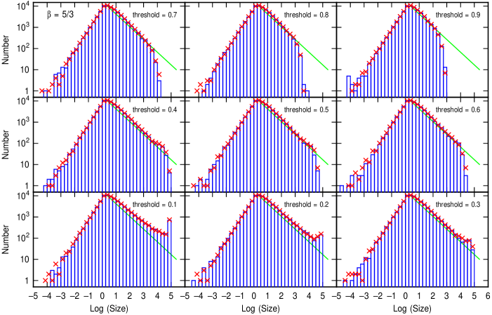
Figure 2: Size spectra of a 1D fBm cloud for different density thresholds. The blue histograms are for the sizes of clumps exceeding the density threshold $C$ and the red crosses are for the sizes of interclump regions with densities less than $1-C$. The slope is independent of density threshold at low size, but the maximum clump size depends on this threshold. The power spectrum slope is $\beta=5/3$ for all thresholds.

Henriksen (1986) also suggested that the IMF comes from counting clumps in a fractal cloud. In his model, the number of clumps per $\log M$ interval is $N(M)\propto L^{-D}$ for fractal dimension $D$ and scale $L$. Combined with a density-size relation, $\rho\propto L^{-D_{\rho}}$, and a definition of mass, $M=\rho L^{D}$, the result is $N(M)\propto M^{-D/\left(D-D_{\rho}\right)}$. For constant density ($D_{\rho}=0$), the geometric result $N(M)\propto M^{-1}$ is recovered. Larson (1982, 1991, 1992) also modeled the IMF for a fractal cloud but assumed $M\propto L$ for linear gas accumulations along filaments; then $N(M)\propto M^{-D}$. Our model is similar to Henriksen’s, but we characterize clouds by their power spectrum slope instead of the fractal dimension, and we consider a fixed density threshold, which makes $M$ effectively proportional to $L^{3}$.

Larson (1973) introduced a slightly different fractal model in which random hierarchical cloud fragmentation produces a log-normal IMF. This model does not have a power-law component because the stellar masses are all at the bottom of the hierarchy, in the same level, and their distribution comes from a spread in the relative number of clumps versus interclump regions that contribute to the final stellar mass during the fragmentation process. Power laws tend to arise when only the fragments can fragment, and log-normals arise when both the fragments and the inter-fragment gas can fragment during a hierarchical process of star formation (Elmegreen, 1985). Detailed models of the first type were in Elmegreen (1997). The present model differs from both of these because we consider only the mass distribution of clumps denser than a fixed threshold, regardless of fragmentation history or level in the hierarchy. We assume no particular fragmentation model at all, only clouds with power-law power spectra.

1.7 Pre-stellar Clumps

Pre-stellar clumps have a density close to the proposed threshold for star formation, and they have about the same mass function as stars. We suggest that pre-stellar clumps get their mass function from fractal cloud structure as shown by our models here. The correspondence between pre-stellar clumps and individual stars is complicated and discussed in Section 4. There is not likely to be a one-to-one correspondence between dense clump mass and stellar mass, because pre-stellar clumps can fragment. Still, the full IMF, including the plateau and the turnover at low mass, might be explained as a result of a combination of processes with cloud structure the main contributor in the power-law part.

The mass function for lower-density clumps, like CO clumps in non-star-forming parts of molecular clouds, are not expected to have the same slope as the dense clumps studied here. CO requires a high column density to form because of molecular line shielding and dust opacity, and it requires a moderately high density for excitation, although CO line emission is possible even at lower densities if the CO line opacity is high. Thus CO clumps should not depend so uniquely on a threshold density as star-forming clumps. With a column density dependence in addition to a density dependence, CO clumps should have a shallower mass function than clumps that are defined entirely by density. This is because massive low-density clumps that would not be included in the mass function with a pure density threshold can be included when there is a column density threshold in addition to a lower and more fuzzy density threshold.

In what follows, Section 2 shows the size distribution functions for clumps in one-dimensional fBm clouds with various power spectrum slopes and threshold densities. Section 3 does the same for three-dimensional fBm clouds in cases with Gaussian density pdfs and lognormal density pdfs. A discussion of the possible relevance of these results and other models linking cloud structure to the IMF is in section 4. It is difficult to make a one-to-one connection between clump mass functions and stellar mass functions because of certain logical inconsistencies. An IMF that arises from a combination of cloud structure and late-state accretion seems to be preferred. In our model, most of the slope in the Salpeter IMF is from the universal geometric structure of turbulent clouds.

2 One-Dimensional Cloud Models

A one dimensional (1D) density strip with a pre-determined power spectrum was made by filling a 1D strip in Fourier space with $(0,1)$ noise multiplied by $k^{-\beta/2}$. After Fourier transforming this $k$-space strip, the result in real space is a density strip with a power spectrum having a slope $-\beta$. In most of the discussion below, we normalized each density strip to have a minimum value of 0 and a maximum value of 1; in some discussions, we normalize them to have a minimum of 0 and an average of 0.5. To make an analogy with cloud mass spectra, we determined the size spectra of the high density regions, i.e., above a fixed threshold density. We also determined the size spectra of the low density regions and of both high and low density regions together. The size distribution is a good representation of the mass distribution because most of a cloud’s mass is at a density close to the threshold value (Elmegreen, 2002, see also Sect. 3 below).

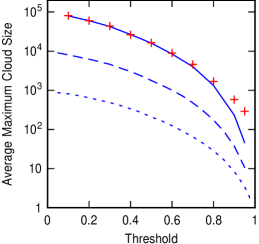
Figure 3: The maximum clump size versus the threshold density used to define a clump. The three lines are for three different total lengths of a 1D fBm cloud.

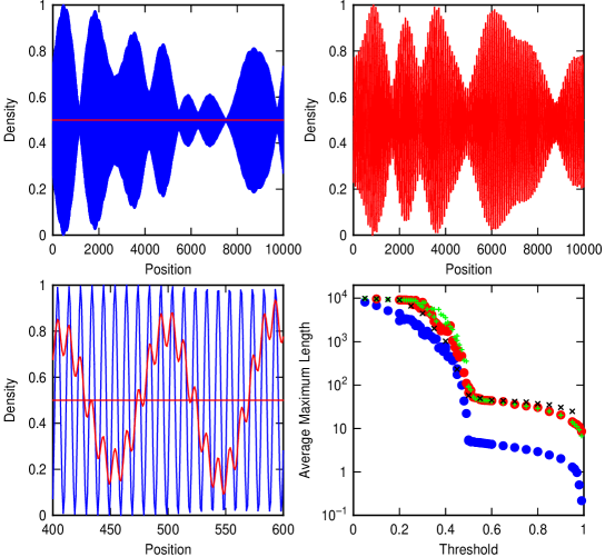
Figure 4: (Top) Two sample density scans with restricted wavenumber ranges. (Lower left) The two scans enlarged and superposed with the same colors as in the top panels. (Lower right) The maximum clump size versus the threshold density for the blue and red scans, in the same colors, and for other composite wavenumbers in black and green.

Figure 1 shows an example. In the top left panel is a random density strip $10^{4}$ pixels long that was made with $\beta=5/3$. The power spectrum of this density strip is in the top right panel, showing the agreement between the slope and the expected $-5/3$ slope. The bottom two panels show blow-up sections of the density strip. A red line indicates a threshold density level of 0.5, and a green line shows the level 0.8. We define a cloud as a region where the density is above a particular threshold level, so there will be one set of clouds with a threshold level of 0.5, and another, smaller set with a threshold of 0.8, etc.. The size of a cloud or intercloud region is the distance between the two points where the density profile meets the threshold value. Clearly there are both large and small clouds at all threshold levels, but there are far fewer clouds that stick above a high threshold level than above a low threshold level.

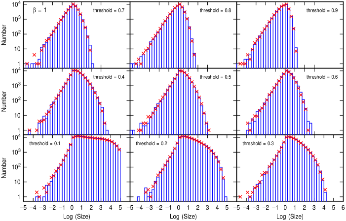
Figure 5: Mass spectra of clumps in 1D fBm clouds with power spectrum slope $\beta=1$ for 8 threshold levels. As in Fig. 2, the blue histograms are for clumps with thresholds $C$ and the red crosses are for interclump regions with thresholds $1-C$.

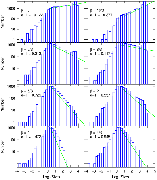
Figure 6: Mass spectra of clumps in 1D fBm clouds with various power spectrum slopes, $\beta$, and a threshold density of 0.5. The slopes of the histograms are indicated by the values of $\alpha-1$ and by the green lines.

Figure 2 shows histograms in blue of the size distribution of clouds for various threshold levels, $C$, and it also shows histogram values, plotted as red crosses, for the size distribution of low-density regions for the corresponding threshold values $1-C$. That is, the cloud size distribution for $C$ is shown in the same panel as the inter-cloud size distribution for threshold $1-C$. Values of $C$ are given in the panels. The clouds and the inter-cloud regions mirror each other in size distributions. This is a sensible result as the density strip is statistically symmetric with respect to inversion from top to bottom. The histograms were made for 1D fBm density strips having $10^{5}$ pixels, and enough strips were made for each $C$ that the number of clouds or inter-cloud regions at a size in pixels with a logarithm between 0 and 0.25 was $10^{4}$ to maintain good counting statistics. In each case, $\beta=5/3$. The green line in the upper mass range has a slope of $-0.6$, for comparison purposes. The rising part of each curve is for sub-pixel sizes.

The maximum size of a cloud decreases with increasing threshold density. Higher thresholds have smaller clouds and larger intercloud regions. Figure 3 shows the trend of average maximum cloud size per simulation versus the threshold level. The solid curve is for fBm strips of $10^{5}$ pixels length, the dashed curve is for strips with $10^{4}$ pixels, and the dotted curve is for strips with $10^{3}$ pixels. These are for densities that are normalized to have a minimum value of 0 and a maximum of 1. For each curve, the maximum cloud size is essentially the whole strip length when the threshold is low, and the maximum cloud size decreases to zero when the threshold is large. The red plus symbols are for a second case where the density strips are normalized to a minimum of 0 and an average of 0.5, with an arbitrary maximum. The maximum cloud sizes are about the same as in the $(0,1)$ normalization except at high thresholds, where the limitless maximum still produces high density regions.

The variation in average maximum length with threshold level may be understood from Fourier analysis. Each density strip is the sum of sines and cosines for a wide range of wavenumbers and for amplitudes that vary with wavenumber as $k^{-\beta/2}$ with $\beta=5/3$ in the cases shown. The short wavelength oscillations modulate the long wavelength oscillations, and so the high intensity part of any long wavelength oscillation has ripples from the short wavelength oscillations. Figure 4 shows an example. The top two panels show the density for the full lengths of $10^{4}$-pixel strips with different Fourier components. The bottom left panel shows the same two strips with the same color coding magnified in the pixel range from 400 to 600. The bottom right panel plots the maximum cloud size versus the threshold level, as in Figure 3, for these two strips. The blue strip in the top and bottom left has wavenumbers only between 1000 and 1010, i.e., it occupies a narrow range in Fourier space with the other Fourier components set to zero. In real space this strip consists of nearly pure oscillations that each go through the midpoint value of 0.5. The range of wavenumbers modulates the amplitude of this oscillation (top left panel) with a beat frequency from the difference in wavenumbers. In this case, the maximum width of a cloud (lower right panel, blue dots) is nearly independent of the threshold level for thresholds larger than 0.5 because each cloud is nearly a pure sine wave. Below a threshold of 0.5, the length of a cloud is the length of the lower envelope of beat frequency oscillation, which is nearly the full strip length, $10^{4}$.

The red strip in the top right and bottom left of Figure 4 has wavenumbers between 100 and 110 and between 1000 and 1010. There is still the high frequency oscillation and modulation of this oscillation as in the blue strip, because the same high frequencies are present, but there is also a low frequency modulation that pushes up and down the high frequency modulation (lower left panel). This low frequency modulation also has a varying amplitude with a beat frequency equal to the difference in wavenumbers (also 10 wavenumbers). Thresholds below 0.5 (lower right panel, red dots) have the same long maximum length as in the blue strip, from the beat frequency, and above this threshold the short length oscillations are seen again. The maximum cloud length at high threshold is higher for the red strip than for the blue strip because the minimum frequency is lower for the red strip. The high threshold lengths are about equal to the number of pixels in the strip, $10^{4}$, divided by $2\pi$ times the minimum $k$ value. For the blue strip, this is $10/2\pi$, or around 2, and for the red strip, this is $100/2\pi$, or around 20.

The green plus symbols in the lower right panel of Figure 4 are for a case where the density strips have wavenumbers only in the range of $100-110$. The black crosses are for a case where the strips have wavenumbers of $100-110$, $310-320$, and $1000-1010$. These two case have about the same maximum cloud lengths versus threshold levels as the red case because the maximum cloud length at high threshold is dominated by the lowest frequencies, which are the same in each case.

The lower right panel of Figure 4 resembles the lower panel of Figure 3, illustrating that the maximum length decreases with increasing threshold because of the isolation of higher frequencies at higher thresholds. The low frequency structure is dominated by beating effects between neighboring frequency groups, and these effects determine the large-scale envelope of the density strip. This is how a cloud length can be greater than half the maximum wavelength in a strip.

Cloud size distributions were also determined for other power spectrum indices using the density normalization from 0 to 1. Figure 5 shows the case $\beta=1$ for a range of threshold densities, and Figure 6 shows histograms for many $\beta$, all with a threshold density of 0.5. The slopes of the high mass parts of the mass functions are indicated in Figure 6 in the upper left corner of each panel and by the green line. These are slopes on the $\log-\log$ plots, and therefore equal to $\alpha-1$. The mass function slope gets more negative as the power spectrum slope gets less negative. This is sensible because more negative mass functions correspond to relatively more low mass clouds, and this corresponds to relatively more high frequency power in Fourier space.

Figure 7 shows the mass function slopes $\alpha$ versus the power spectrum slopes $\beta$ for the 1D fBm clouds. The data fit the relation $\alpha=2.83-0.66\beta$ between $\beta=4/3$ and $11/3$. The threshold value was 0.5 for this. Higher thresholds would not change the result much because the slope $\alpha$ is independent of the threshold below the upper clump mass (which does depend on the threshold). According to Stützki et al. (1998) and Hennebelle & Chabrier (2008), the relation is $\alpha=3-\beta/\gamma$ for $\gamma$ equal to the power in the mass-radius relation. In our 1D case, $\gamma=1$ and this equation would suggest $\alpha=3-\beta$. Our actual result is close to this.

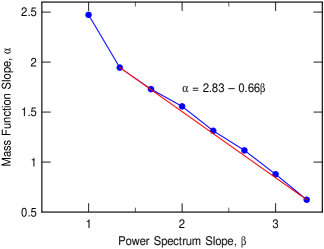
Figure 7: The slope of the clump mass function versus the slope of the power spectrum for 1D fBm clouds with a threshold for clump definition equal to 0.5.

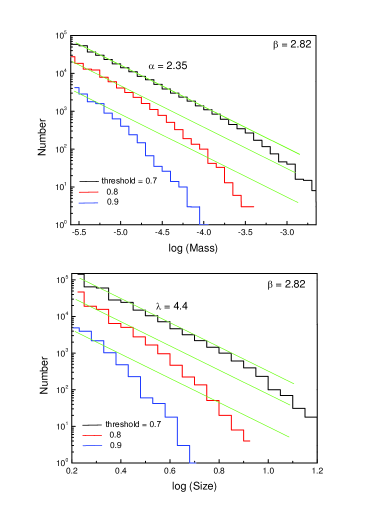
Figure 8: Mass and size functions for 3D fBm clouds with Gaussian pdfs. The power spectrum slope is $2.82$, which produces a mass function similar to the Salpeter IMF for low and intermediate masses. The drop in the mass spectrum for high mass and high threshold density is a result of a superposition of low and high frequency wavenumbers in the fBm cloud, as discussed in Figure 4. Green lines are fitted to the low mass and size portions of the distributions.

3 Three Dimensional fBm Models

Clump mass functions were also determined for three-dimensional clouds with and without log-normal density pdfs. The log-normal was made to resemble isothermal clouds in simulations of MHD turbulence Vazquez-Semadeni (1994). For 3D, we calculated clump mass in addition to volume, although the mass turned out to be nearly equal to the volume multiplied by the threshold density in all cases, as assumed above for the 1D experiments.

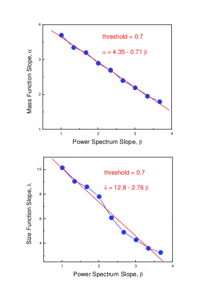
Figure 9: The slopes of the low mass and low size parts of the mass and size functions are shown versus the power spectrum slopes for 3D fBm clouds with a density threshold for clumps equal to $0.7$.

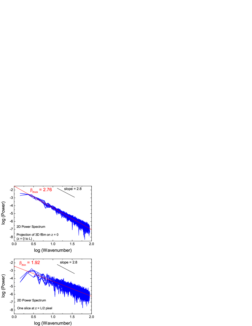
Figure 10: (Top) Power spectrum of a 3D fBm density field made by the integrating the density along the z axis from $z=0$ to $L$ (the size of the box in pixels). (Bottom) Power spectrum of the density field of a slice at $z=L/2$ with one pixel thickness. The slope of the power spectrum of a 3D fBm density field is shown at the top of each panel. The projected power spectrum has about the same slope as the 3D power spectrum, but the slice has a slope that is shallower by about 1.

The clouds were made in several steps. First we filled a $256^{3}$ cube in wavenumber space with random complex numbers, $(k_{x},k_{y},k_{z})$, uniformly distributed from $0$ to $1$. Then we multiplied each number by $k^{-\beta/2}$, where $k=(k_{x}^{2}+k_{y}^{2}+k_{z}^{2})^{1/2}$. We took the inverse Fourier transform of this cube to make a real space density distribution $\rho_{\rm fBm}(x,y,z)$. This distribution is a standard fBm cloud, and it has a power spectrum with a negative slope $\beta$. Some of the clump mass functions presented below use this fBm cloud. To make a log-normal density pdf, we exponentiated this result:

$$\rho_{LN}(x,y,z)=\exp(\rho_{\rm fBm}(x,y,z)/\rho_{0}),$$ (1)

where $\rho_{0}$ is for normalization. To build up the statistics of the cloud mass and size distributions, we generated an ensemble of $\sim 100$ fBm distributions for each of the three normalizations discussed below. Clumps are defined as connected pixels above a threshold density inside the overall cloud. The clump mass is the sum of the density values in all of these connected pixels, and the clump size is the cube root of the number of pixels.

3.1 fBm clouds with Gaussian density pdfs

Figure 8 shows the mass and size distributions for clumps in standard fBm clouds with Gaussian density pdfs in the case where $\beta=2.82$. This $\beta$ was chosen because it gives a mass function slope similar to the Salpeter IMF at a cloud-defining minimum density of 0.7. Three threshold densities are considered. The low mass and small size parts of the clump functions have about the same slope for all threshold densities, and there is a steepening of the functions at intermediate mass and size. This steepening occurs at smaller masses and sizes when the threshold density is higher, as for the 1D results.

Figure 9 shows the slopes of the low-mass parts of the clump mass and size distribution functions versus the power spectrum slope, $\beta$, for a density threshold of 0.7. There is a decreasing trend as for the 1D case. Steeper power spectra produce shallower mass and size distribution functions. The slope of the Salpeter mass function is $\alpha=2.35$ on this plot, and that is associated with $\beta=2.82$. This is the 3D $\beta$ in the cloud volume. The relation between the two quantities is $\alpha=4.35-0.71\beta$ for a threshold of 0.7. Recall that the Stützki et al. (1998) and Hennebelle & Chabrier (2008) result for 3D with $\gamma=3$ is $\alpha=3-0.33\beta$.

3.2 Comparison between our Model and the Press-Schechter or Hennebelle-Chabrier Models

The decrease in $\alpha$ with increasing $\beta$ in Figure 9 is opposite to the trend in Press & Schechter (1974) because of a difference in the definition of clumps. In Press & Schechter (1974) and in Hennebelle & Chabrier (2008), a clump is defined as an object with an average density above a threshold $\rho_{c}$. The clump mass is the sum of the masses of only the dense parts ($\rho>\rho_{c}$) of this clump. Generally, the clump contains both high density ($\rho>\rho_{c}$) and low density ($\rho<\rho_{c}$) parts, and the high-density mass is taken equal to the total mass multiplied by the probability that the density is high. This probability is the integral over the density pdf for all densities above the threshold. The density pdf is written as $(2\pi\sigma^{2})^{-0.5}\exp(-0.5\delta_{c}^{2}/\sigma^{2})$ for dispersion $\sigma^{2}=(2\pi)^{-3}\int_{k_{min}}^{k_{max}}P(k)dk^{3}$ and power spectrum $P(k)\propto k^{-\beta}$ (Padmanabhan 1993). Evidently, $\sigma\propto k^{(3-\beta)/2}\propto M^{(\beta-3)/6}$, as discussed in the Introduction. For $\beta<3$, the integral for $\sigma$ depends only on the upper boundary, $k_{max}$, and includes all $k<k_{max}$. As $M$ increases, this upper boundary decreases and the range of $k$ decreases as well. This is why the dispersion of the pdf, which depends on the range of $k$, decreases with increasing $M$ when $\beta<3$. For $\beta>3$, the integral for $\sigma$ depends only on the lower boundary, $k_{min}$, and includes only $k>k_{min}$ up to some cutoff in $k$, which may be viewed as the inverse of a smoothing length. As $M$ increases, the lower boundary to $k$ decreases, increasing the range of $k$ between that lower boundary and the upper cutoff in $k$. As a result, the dispersion $\sigma$ increases – opposite to the trend for $\beta<3$.

Writing either of these two $k$ limits in terms of $M$, the clump mass function equals $n(M)\propto(M^{2}\sigma)^{-1}\exp(-0.5\delta_{c}^{2}/\sigma^{2})$, so the power law part at low $M$ has a slope $\alpha=1.5+\beta/6$. This is the Press & Schechter result. The probability that the density is high inside a region increases with increasing region mass for $\beta<3$ and decreases with increasing region mass for $\beta>3$, in proportion to $\sigma^{-1}$ at low $M$ (where the exponential is not important). In the first case, $\beta<3$, this means that clumpy regions have dense-gas masses that progressively get smaller than in the purely hierarchical mass function ($M^{-2}$) as $M$ decreases. As a result, the clump mass function is shallower than $M^{-2}$ when $\beta<3$ in the Press & Schechter formulism. (Visualize an $M^{-2}$ mass function that shifts to lower $M$ at low $M$ and higher $M$ at high $M$, stretching horizontally on such a plot.) Similarly in the case $\beta>3$, clumpy regions have progressively more mass than in the $M^{-2}$ function as $M$ decreases, making the mass function steeper (visualize the same initial $M^{-2}$ function, but now compress it horizontally). This is opposite to the trend in Figure 9. Physically, what is happening is that the density distribution is smoother (smaller $\sigma$) at larger $M$ when $\beta<3$, so a region with average density exceeding some threshold has fewer and smaller dips to sub-threshold density inside of it. Nearly the entire enclosed mass is then counted. Smaller mass regions for $\beta<3$ have large density fluctuations inside of them, so that even when the average density exceeds the threshold, there are still a lot of regions and a lot of mass at densities less than the threshold. In this case, the mass fraction above threshold is small.

Another difference between our model and that of Press & Schechter (1974) or Hennebelle & Chabrier (2008) concerns the lower limit to the mass. For $\beta<3$, this lower limit is important, as discussed above. In the Press & Schechter formulism, the region defined to be a clump does not depend much on the resolution scale, which is the lower limit to $M$. Clump regions stay about the same as the resolution increases, and all that happens is that clump masses get more accurate. That is, smaller scale structure occurs near the density threshold and the pdf provides a more detailed representation of the fraction of the mass above threshold. In our model, the definition of each clump changes as the map resolution increases. More clumps and smaller clumps appear above the density threshold at higher resolution and some massive clumps disappear as they pick up fine-scale subregions below threshold. On the other hand, the mass function slope is independent of resolution in our model. Higher resolution extends the mass function to lower mass and changes the total count of clouds for fixed mass above the density threshold, but it leaves the mass function slope the same.

Physically, our model applies when only the dense parts of a cloud complex are identified as clumps. These clumps can have highly irregular shapes, like filaments, but they cannot include multiple islands of threshold density gas separated by lower-density inter-island gas. Our model would identify each island as a separate clump. In Press & Schechter (1974) and Hennebelle & Chabrier (2008), entire regions with islands and inter-island gas are counted as single clumps if the average density of it all exceeds the threshold. In all cases, the total mass in the mass function comes only from the parts of the clumps that are above the density threshold; only the definition of a clump and the counting of clumps differ. Which clump definition more accurately applies to pre-stellar clumps depends on how observers define their clumps and the masses of their clumps. While this may seem like a small detail, the slope of the clump mass spectrum, $\alpha$, depends on the slope of the power spectrum, $\beta$, in opposite ways in these two cases. If clump finding algorithms change their identification of clumps as the spatial resolution increases, calling what used to be a single clump at low resolution two separate clumps at higher resolution, then our definition of clumps would apply.

3.3 Projected Clouds

Observations do not generally determine the 3D power spectrum of density in a 3D cloud, but rather the 2D power spectrum of projected density in a 3D cloud. This difference between the observed and the intrinsic power spectra has to be investigated before we link the observed power spectrum to a 3D clump mass function. Two-dimensional power spectra were determined for the projected density distributions and for thin slices in 3D fBm clouds. According to equation (28) in Lazarian & Pogosyan (2000), the slope of the 2D power spectrum of projected density, $\beta_{\rm thick}$, integrated along a thick path through a 3D cloud, should be equal to the slope of the power spectrum in the original 3D cloud, $\beta$. The slope of the power spectrum of a thin slice in a 3D cloud, $\beta_{\rm thin}$, should differ by 1 from the 3D slope: $\beta_{\rm thin}=\beta-1$. The power spectrum is shallower for a thin slice than a projection because the thin slice has more fine-scale structure. Figure 10 shows these 2D power spectra for a 3D fBm cloud with $\beta=2.8$. The thick path projection through a 3D fBm cloud (top panel) was determined by integrating along the $z$ axis from $z=1$ to $z=L$, which is the 3D box size. The thin slice projection (bottom panel) was determined by using only the $z=L/2$ position to make the 2D map. Figure 10 indicates that the 2D power spectra have approximately the slopes that are expected. The projected density field has a 2D power spectrum slope $\beta_{\rm thick}=-2.76$, and the 2D power spectrum of the thin slice has a slope $\beta_{\rm thin}=1.92$. These are approximately equal to, and 1 less than, respectively, the 3D slope of $\beta=2.8$.

This result for 2D indicates that observation of 2D power spectra for projected or line-of-sight integrated clouds having slopes of about $-2.8$ (Table 1) correspond to 3D power spectra inside those clouds with about the same slope. Correspondingly, Figures 8 and 9 now suggest that for this slope, the mass function of clumps has a slope equal to the Salpeter value, $\alpha=2.35$. Thus the power-law portion of the stellar IMF can have its fundamental origin in the geometric structure of clouds. Section 4 discusses the implications of this point in more detail.

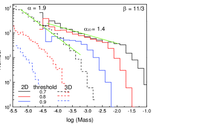
Figure 11: Projected mass functions of clumps in 3D fBm clouds obtained by integrating along the $z$ axis. The mass spectra are shown by solid lines for thresholds of $0.7$, $0.8$ and $0.9$. The mass functions of the corresponding 3D fBm clouds are shown by dashed lines. The power spectrum slope is $\beta=11/3$. Green lines are fitted to the 2D and 3D mass functions for a density threshold of $0.7$.

Mass functions for clumps observed in projection are shown in Figure 11. These were made from the same 3D fBm clouds used for Figure 9, but the search algorithm was done on 2D projections of the clouds made by integrating along the $z$ axis. Mass functions for the 3D fBm clumps shown previously are reproduced as dashed lines. Three different density thresholds are considered with a 3D power spectrum slope $\beta=11/3$. This is the slope of the 3D power spectrum for velocity in classical 3D incompressible Kolmogorov turbulence. The green lines in Figure 11 show fits for a density threshold of $0.7$. As for the 3D mass functions, the slopes of the low-mass parts of the 2D mass functions are about the same for all density thresholds; the slopes of the upper mass parts are steeper, and the upper mass limits are smaller, for higher density thresholds. The slope of the 3D mass function is written in the Figure as $\alpha=1.9$. This is also the value expected from Figure 9 for $\beta=11/3$. The slope of the projected 2D mass function is $\alpha_{\rm 2D}=1.4$. Evidently, the 2D mass function of the projected 3D cloud is shallower than the 3D mass function in the unprojected cloud by $\sim 0.5$ in the slope. This implies that the 2D mass function has proportionally more high mass clumps, presumably from the blending of smaller clumps.

The 2D mass function of projected clumps is not necessarily the same as the mass function of interstellar clouds observed with dust emission integrated along a long line of sight. If there is blending on the line of sight because each clump is relatively large in angle, as would result from a low threshold density for the definition of a clump, then this projection result might apply. However, if the density threshold is very high and there is no blending for a cloud with a finite line-of-sight path length, then the observed projected mass function could be closer to the true 3D mass function.

3.4 fBm clouds with log-normal density pdf’s

A second set of models was made with log-normal density pdfs, which are exponentials of the previously discussed fBm clouds (Equation 1; see also Elmegreen (2002)). We considered three types of density normalization. The first forced each log-normal cloud to have a minimum density, $\rho_{\rm LN}$, of 0 and a maximum density of $e^{1}$. This was done by selecting $\rho_{0}$ in equation (1) to be the maximum value of $\rho_{\rm fBm}$, designated as $\rho_{\rm fBm,max}$. Each fBm cloud had a different $\rho_{0}=\rho_{\rm fBm,max}$. Clumps were defined to be regions where the density $\rho_{\rm LN}$ was larger than some fixed fraction, $f_{\rm clump}$, of the peak value of $e^{1}$. The same fraction was used for all of the log-normal distributions in the ensemble; different $f_{\rm clump}$ were used to see how the mass distribution depended on the threshold density.

A second case of $\rho_{\rm LN}$ normalization had a minimum density of 0 and a different maximum density for each cloud. The normalization $\rho_{0}$ was now taken to be the same for each cloud and equal to the average of all the $\rho_{\rm fBm,max}$ from the 100 previous ensembles, $\rho_{0}=<\rho_{\rm fBm,max}>$. Thus the density maximum in a log-normal cloud was $\rho_{\rm LN,max}=\exp(\rho_{\rm fBm,max}/<\rho_{\rm fBm,max}>)$. The random numbers were the same as in the first case. The density threshold for the definition of a clump was set equal to a fraction $f_{\rm clump}$ of each density peak, i.e., $f_{\rm clump}\rho_{\rm LN,max}$. Because the density peaks are all different in this normalization, the density thresholds are all different too, although the density threshold fractions are the same. The fractions are taken to be the same as in the first normalization case, with a different $f_{\rm clump}$ for each ensemble of 100 clouds.

The third case of $\rho_{\rm LN}$ normalization had a minimum density of 0 and a variable maximum $\rho_{\rm LN,max}$ defined in the same way as in the second case, i.e., with the same $\rho_{0}=<\rho_{\rm fBm,max}>$ for each cloud. Now the density threshold to define a clump was taken to be the same for each cloud, not variable with the same fraction of the peak.

The motivation for considering these different cases is our hypothesis that cloud collapse to stars begins to get significant at a certain characteristic density where the microscale processes change (Elmegreen, 2007). We would like to know, for example, how the clump mass spectrum depends on the peak gas density in a kpc-size region for a fixed characteristic density (this is closest to case 3). We would also like to know how it depends on the relative density of the collapse threshold (close to case 2). If the absolute density for the onset of collapse is the same everywhere, then the timescale for collapse would be about the same and the star formation rate should scale as the first power of the average ISM density. If, on the other hand, the relative density for collapse is the same everywhere, then the timescale will scale with the inverse square root of the average density and the star formation rate will scale with the 1.5 power of the average density.

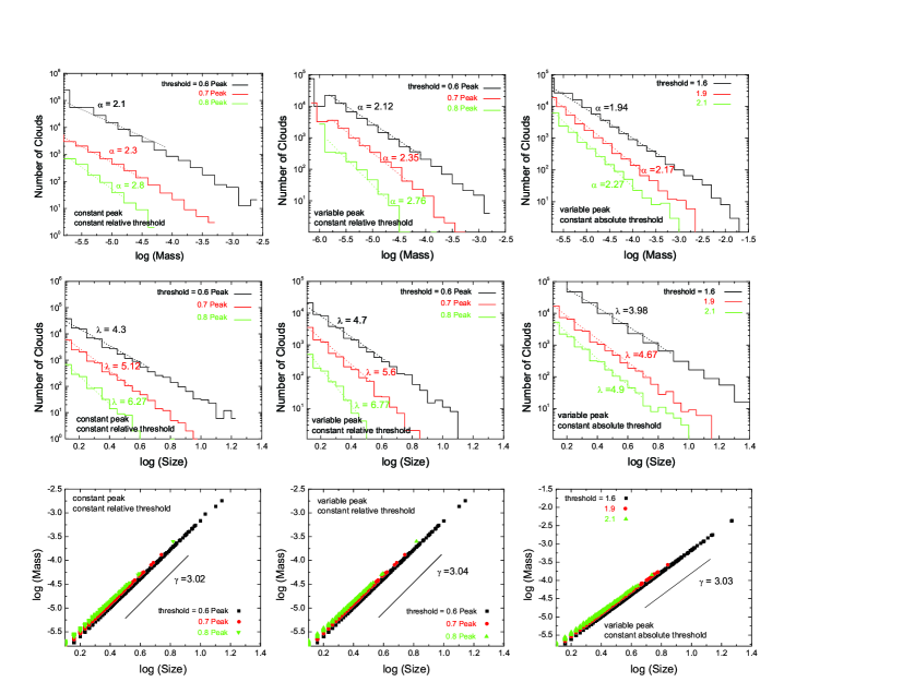
Figure 12: (Top) Clump mass spectra of 3D fBm clouds with log-normal density pdfs and power law slopes $\beta=2.8$. Three threshold values equal to $0.6$, $0.7$ and $0.8$ are considered. (Middle) Size distributions of the clumps. (Bottom) The mass-size relations. The three methods for cloud normalization, corresponding to the three columns, are described briefly in each panel and discussed in the text.

Figure 12 shows the mass and size distributions and the mass-size relation for the three different cases using $\beta=5/3$. Each curve in the top two rows is a different clipping level, with lower levels producing larger numbers of clumps. The clipping levels were chosen to avoid excessive cloud merging at low levels and too few clouds at high levels. Each dot in the lower row represents a single clump. Lower clipping levels produce lower mass clouds for the same size.

The mass and size distributions are related to each other by the mass-size correlation. For mass distribution $dn(M)/dM=M^{-\alpha}$, size distribution $d\Lambda(R)/dR=R^{-\lambda}$, and mass-size relation $M\propto R^{\gamma}$, we should have $dn(M)/dM=(d\Lambda(R)/dR)(dR/dM)$, from which we get $\alpha=1+(\lambda-1)/\gamma$. The bottom panels of Figure 12 indicate that $\gamma\sim 3.0$ for all cases, which implies that the average density of clouds is nearly uniform when there is a threshold density to define the clouds. This average density is approximately 1.08 times the threshold density, depending a little on $\beta$, because most the cloud volume is near the cloud edge where the density equals this threshold. Recall that clumps made from fBm clouds are fractals with convoluted surfaces near the threshold density, so a higher fraction of the mass is near this threshold density than in an isothermal sphere. For $\gamma=3.0$, $\alpha=1+0.33(\lambda-1)$. All of our 3D results approximately follow this expression.

The mass functions and size functions in 3D resemble those in 1D and in the regular fBm case in the sense that they have similar slopes at low mass but then steepen to different degrees at high mass. The mass where the steepening begins is lower for higher threshold densities. This trend is present for all three cases in Figure 12. The average slope of the mass function is a blend of the common low-density slope and the steepened high-density slope. This average steepens from $-2.1$ to $-2.8$ as the relative threshold density increases from $0.6$ to $0.8$ in the first normalization case. The average slope steepens in the second case from $-2.12$ to $-2.76$ and in the third case from $-1.94$ to $-2.27$.

The steepening with increasing threshold density is lowest in the third case, which is the one with a variable peak and a constant threshold for clump definition. The variable relative density threshold that results in this case effectively blends together the mass functions from cases with higher and lower absolute thresholds.

4 Discussion: How important is Cloud Structure to the IMF?

As a step toward understanding the IMF, we have investigated the mass functions of clumps that exceed a threshold density in fractal Brownian motion clouds. We expected that mass functions will resemble volume functions when there is a threshold density, and we verified that here. We also found relations in 1D and 3D between the slopes of the power laws for the mass functions and the power spectra, reminiscent of the analytical results in Stutzki, et al. (1998) and Hennebelle & Chabrier (2008), although not exactly the same. For the most realistic case, a 3D fBm cloud with a projected power spectrum similar to what is observed in molecular clouds, the mass function of clumps denser than a threshold is a power law with the Salpeter slope. This result does not depend on the threshold density much, nor on the projection. Only the maximum clump mass depends on the threshold density. As a result of this agreement between the clump mass spectrum and the stellar IMF for realistic structure in interstellar clouds, we are led to believe that the power-law part of the IMF results in large part from cloud structure at a threshold density. The low-mass part of the IMF would then arise from an inefficiency of star formation below a certain mass, like the thermal Jeans mass. We consider this in more detail here.

The clump function is a reasonable starting point for studies of the IMF, but the IMF cannot be explained so simply. If there is a fixed density threshold (e.g., Johnstone et al., 2004; Elmegreen, 2007), then larger clumps with the same temperature contain more Jeans masses and should fragment into more sub clumps and stars. The assumed one-to-one correspondence between clump mass and star mass is lost. This is a problem faced by observations of the pipe nebula (Rathborne et al., 2009): the clump mass distribution resembles the IMF, but the largest clump contains many stars and breaks the assumption of a one-to-one correspondence between clump mass and star mass. On the other hand, if there is such a correspondence, i.e., if the Jeans mass scales with the clump mass, then massive stars form in lower density clumps or in the low-density periphery of clumps (in the absence of temperature variations), and this positioning is contrary to the observed mass segregation in young clusters. More physical processes are required, such as heating.

An additional problem is that if larger clumps contain more Jeans masses and form more stars, then there would be a stellar mass function inside each clump, which could, in principle, differ from the clump mass function. Only the sum of the IMFs inside all of the clumps has to equal the total cloud IMF, which is the generally observed function. There is virtually no systematic study of individual (local) IMFs inside embedded-star clumps.

There are several ways in which the sum of individual clump IMFs can give the observed IMF. One is for the IMF inside each clump (the ”internal clump IMF”) to be the same as the cluster IMF, up to a certain maximum star mass dependent on the clump mass, and for the clump mass function to have a slope shallower than or equal to $\alpha=2$ (Elmegreen, Elmegreen, Chandar, Whitmore & Regan, 2006). This seems ruled out by the observation of clump mass functions with steeper slopes, similar to that of the IMF. A steeper clump function produces a summed IMF that is steeper than the individual clump IMF (see below).

Another way to give the right summed IMF is for the internal clump IMF to be a random sample of the cluster IMF up to arbitrarily high stellar mass in each clump. Then the clump mass function does not enter into the IMF. However, it is unrealistic to expect each clump to be able to produce a star of arbitrarily large mass. With additional physical processes, such as continued accretion from other clumps, random IMF sampling might be possible, but not with static clumps as the only reservoirs for internal clump IMFs.

In a third way, the internal clump IMF can be an arbitrary function of the star-to-clump mass ratio. Then the summed IMF will have the same power as the clump mass function in the power-law range, regardless of the internal clump IMF. In this third case, the universality of the IMF follows from the universality of cloud structure. The present study of fBm clump mass functions fits closest to this third scenario. There need not be a one-to-one correspondence between clump mass and star mass. Instead, there has to be an internal IMF for each clump that is relative, i.e., the stellar masses scale up or down with the clump mass. This might be the case if competitive accretion dominates the assembly of stars inside each clump, and if heating, merging, ejection, and other processes contribute to the final stellar IMF inside each clump, regardless of what that IMF is, as long as all of the rates and masses are proportional to the clump mass.

These three scenarios are worth reviewing here. We consider in all cases a constant ratio of total star mass to clump mass in each clump, so the total star mass in each clump is equal to some fraction $\epsilon$ of the clump mass. We also consider for simplicity only the power-law part of the IMF, ignoring the low-mass plateau. The clump mass function is $dn_{c}(M_{c})/dM_{c}=n_{c0}M_{c}^{-\alpha}$, as before.

For the first of the three scenarios, we consider a star mass function inside each clump of $dn_{s}(M_{s})/dM_{s}=n_{s0}M_{s}^{-1-x}$ for Salpeter $x=1.35$. The integral of $M_{s}$ times the star mass function from a fixed minimum stellar mass $M_{s,min}$ up to some very large stellar mass has to equal the total stellar mass in the clump, which is $\epsilon M_{c}$. That means $n_{s0}=A\epsilon M_{c}$ for $A=(x-1)M_{s,min}^{x-1}$, and it means the IMF in a clump of mass $M_{c}$ is $n_{s}(M_{s}|M_{c})=A\epsilon M_{c}M_{s}^{-1-x}$. The summed star mass function for all of the clumps is the integral of $M_{s}n_{s}(M_{s}|M_{c})$ over the clump mass function from the minimum clump mass that is likely to contain a star of mass $M_{s}$, which is $M_{c,min}=xM_{s}^{x}/\left(A\epsilon\right)$, up to the maximum clump mass in the cloud, $M_{c,max}$. The minimum clump mass comes from the requirement that $\int_{M_{s}}^{\infty}n_{s0}M_{s}^{-1-x}dM_{s}=1$. The summed star mass is therefore

$$n_{sum}(M_{s})=\int_{M_{c,min}}^{M_{c,max}}A\epsilon M_{c}M_{s}^{-1-x}n_{c0}M_{c}^{-\alpha}dM_{c}$$

$$={{A\epsilon n_{c0}M_{s}^{-1-x}}\over{2-\alpha}}\left(M_{c,max}^{2-\alpha}-\left[{{xM_{s}^{x}}\over{A\epsilon}}\right]^{2-\alpha}\right)$$ (2)

for $\alpha\neq 2$. For $\alpha=2$, it is

$$n_{sum}(M_{s})=A\epsilon n_{c0}M_{s}^{-1-x}\ln\left(A\epsilon M_{c,max}/\left[xM_{s}^{x}\right]\right).$$ (3)

When $\alpha\leq 2$, the first term in the parenthesis of equation (2) dominates the second and the summed stellar mass function is $\propto M_{s}^{-1-x}$, which is the same as the individual clump IMF. If $\alpha=2$, the same is true approximately, with only a logarithmic deviation. If $\alpha>2$, then the second term in the parentheses of equation (2) dominates the first, and the summed IMF is $\propto M^{-1-x(\alpha-1)}$. This summed IMF can be much steeper than the Salpeter function if $\alpha>2$ (Kroupa & Weidner, 2003). Because dense clumps are observed to have $\alpha>2$, individual clump IMFs have to be shallower than the whole-cluster IMF, which is the Salpeter function.

For the second of the three scenarios, a star of any mass is supposed to be able to form in a clump of any mass, in which case $M_{c,min}$ is constant in the integral of equation 2, independent of $M$. Then the summed IMF is trivially proportional to the individual clump IMF, $M_{s}^{-1-x}$.

The third scenario allows a variety of stellar mass functions inside each clump and always gives a summed stellar function with a slope that is equal to the slope of the clump mass function. To demonstrate this, we assume the internal clump IMF is a distribution function, $P(f)df$, of the ratio of star mass to clump mass, $f=M_{s}/M_{c}$ for $f$ between $f_{min}$ and $f_{max}$. For simplicity, $P(f)=P_{0}f^{-p}$. Then the summed stellar mass function is

$$n_{sum}(M_{s})=\int_{f_{min}}^{f_{max}}P(f)n_{c}(M_{c})df$$

$$=\int_{M_{c,min}}^{M_{c,max}}P_{0}M_{s}^{1-p}M_{c}^{p-\alpha-2}dM_{c},$$ (4)

which integrates to

$$n_{sum}(M_{s})={{P_{0}M_{s}^{1-p}}\over{(p-\alpha-1)}}\left(M_{c,max}^{p-\alpha-1}-M_{c,min}^{p-\alpha-1}\right).$$ (5)

If clumps larger than a certain mass $M_{J}$ fragment into stars, then $M_{c,min}=MAX(M_{J},M_{s}/f_{max})$. Also, $M_{c,max}=M_{s}f_{min}$.

Now consider clump masses larger than the fragmentation limit, i.e. $M_{s}/f_{max}>M_{J}$. Then $M_{c,min}=M_{s}/f_{max}$, and the stellar mass function is

$$n_{sum}(M_{s})={{P_{0}M_{s}^{-\alpha}}\over{(p-\alpha-1)}}\left(f_{min}^{(1+\alpha+p)}-f_{max}^{(1+\alpha-p)}\right).$$ (6)

This IMF is proportional to $M_{s}^{-\alpha}$, which is the same as the clump mass function with a slope that is independent of the individual clump IMF slope $p$. Below the fragmentation limit but not as low in stellar mass as the minimum fragment size, we have $M_{c,min}=M_{J}$ and also $M_{s}>M_{J}f_{min}$. Then

$$n_{sum}(M_{s})={{P_{0}M_{s}^{1-p}M_{J}^{(p-\alpha-1)}}\over{(1+\alpha-p)}}$$

$$\times\left(1-\left[{{M_{J}f_{min}}\over{M_{s}}}\right]^{(1+\alpha-p)}\right),$$ (7)

where the second term in the brackets is less than the first for $1+\alpha>p$. In this case, the summed IMF is proportional to $M_{s}^{1-p}$, which is the function $P(p)$ in intervals of $\log P$.

This result for the third scenario implies that if clumps need to contain at least one Jeans mass before they fragment into a little sub-cluster, and if the Jeans mass, $M_{J}$, is about the same for all clumps (i.e., for a constant temperature and threshold density), then the summed IMF above $M_{J}f_{max}$, which is the largest star that comes from an $M_{J}$ piece, is a power law with the same slope as the clump mass function. Below $M_{J}f_{max}$, the summed IMF is the internal clump mass function. If $p\sim 2$, then the IMF plateau may be explained as the part below the smallest unstable clump. It would be composed of stars coming from that smallest unstable clump, and from other clumps with slightly larger masses (Elmegreen, 2000).

What type of model will produce a relative stellar mass function, $p(f)$, inside each clump, rather than an absolute stellar mass function inside each clump? Such a function would seem to result from self-similar processes that scale to the clump mass, and that would include protostellar accretion of a gas mass proportional to the clump mass, and protostellar interactions, including possibly coalescence. As all of this occurs in clumps more massive than $M_{J}$, the motions would be transonic and $M_{J}$ itself would be unconnected with the final star mass. Note that in this model, the number of fragments in a clump would not be proportional to the number of $M_{J}$ in the clump, because that would give stellar masses that are centered around $M_{J}$ rather than stellar masses that scale with the clump mass. In this interpretation, $M_{J}$ enters the final IMF in its establishment of a minimum fragmentable clump mass at the IMF plateau. Also in this model, massive clumps would not produce more stars than low-mass clumps with the same average stellar mass, but they would produce the same number of stars as the low-mass clumps and a higher mass for each star. Thus the third model is like assuming each clump produces stars with masses proportional to the clump mass. It is effectively the same as assuming a one-to-one correspondence between clump mass and star mass, even though each clump forms several stars with a local, and even arbitrary, relative IMF.

5 Conclusions

Interstellar clouds have a power spectrum of column density that is a power law with a negative slope in the range from $\sim 2.7$ to 3. The underlying structure is not a clump-interclump medium but a continuum of densities with structures in the form of sheets, filaments, and clumps. Surveys that are sensitive to column density or density view these clouds as collections of discrete clumps, which are the densest parts of the continuum. In many models, star formation also selects the densest parts of a cloud. Here we investigated a model for the IMF based on this principle. We determined clump mass spectra above threshold densities for clouds with power-law power spectra. The results showed a dependence of the clump mass spectrum on the slope of the power spectrum, as expected from analytic theory, and a trend toward decreasing maximum mass with increasing relative threshold density. For realistic power spectra, an IMF-like slope results for the derived clump spectra. At a very basic level, this result supports numerous models of star formation where the intermediate-to-high mass part of the IMF has its basic form from cloud geometry.

The IMF has to be more complicated than this, however. If there is a characteristic density for star formation and a wide range of clump masses above that density, as is the case for clouds with power-law power spectra, then larger clumps contain more unstable sub-clumps and should form more stars or more massive stars. If they just form more stars with the same characteristic mass, e.g., the thermal Jeans mass, then the assumed connection between clump mass and star mass is lost, as is the connection between the clump mass function and the IMF. The IMF needs a different origin in that case. If, on the other hand, the average star mass inside a clump scales with the clump mass, then the clump mass spectrum can be the same as the IMF in the power-law part. Such scaling allows for the interesting possibility that clumps have internal IMFs that are different from observed IMFs in whole clusters, which is the sum from many clumps. Internal IMFs inside clumps have not been investigated much so this possibility remains open.

Competitive accretion and clump coalescence play an important role in forming the IMF, as shown by many numerical simulations. These processes usually operate along with cloud fragmentation, so it is unclear whether the bulk of the IMF power law still comes from geometry. That is, the basic $dn/dM\propto M^{-2}$ power law that arises in so many fragmentation models is already very close to the IMF (the Salpeter slope is $=-2.35$ in this convention). Accretion, stellar winds, coalescence, and other microphysics need only modify this initial function by a small amount, giving a slight bias toward lower mass objects. Experiments of competitive accretion in clouds with different density power spectra or in uniform clouds might reveal the overall importance of cloud geometry in the IMF.

References

- Bastian et al. (2010) Bastian N., Covey K. R., Meyer M. R., 2010
- Bate (2009) Bate M. R., 2009, MNRAS, 397
- Bate et al. (2002) Bate M. R., Bonnell I. A., Bromm V., 2002, MNRAS, 332
- Bensch et al. (2001) Bensch F., Stützki J., Ossenkopf V., 2001, A&A, 366
- Beresnyak et al. (2005) Beresnyak A., Lazarian A., Cho J., 2005, ApJ, 624
- Bonnell et al. (2001) Bonnell I. A., Bate M. R., Clarke C. J., Pringle J. E., 2001, MNRAS
- Bonnell et al. (2008) Bonnell I. A., Clark P., Bate M. R., 2008, MNRAS, 389, 1556
- Bonnell et al. (2001) Bonnell I. A., Clarke C. J., Bate M. R., Pringle J. E., 2001, MNRAS
- Bonnell et al. (2007) Bonnell I. A., Larson R. B., Zinnecker H., 2007, Protostars and Planets V, pp 149–164
- Boulanger et al. (1990) Boulanger F., Falgarone E., Puget J. L., Helou G., 1990, ApJ, 364, 136
- Clark & Bonnell (2006) Clark P. C., Bonnell I. A., 2006, MNRAS, 368, 1787
- Clark et al. (2008) Clark P. C., Bonnell I. A., Klessen R. S., 2008, MNRAS, 386, 3
- Clark et al. (2009) Clark P. C., Glover S. C. O., Bonnell I. A., Klessen R. S., 2009, ArXiv e-prints
- Clark et al. (2007) Clark P. C., Klessen R. S., Bonnell I. A., 2007, MNRAS, 379, 57
- Crovisier & Dickey (1983) Crovisier J., Dickey J. M., 1983, A&A, 122, 282
- Deshpande et al. (2000) Deshpande A. A., Dwarakanath K. S., Goss W. M., 2000, ApJ, 543, 227
- di Fazio (1986) di Fazio A., 1986, A&A, 159, 49
- Dib et al. (2008) Dib S., Brandenburg A., Kim J., Gopinathan M., André P., 2008, ApJL, 678, L105
- Dib et al. (2010) Dib S., Shadmehri M., Padoan P., Maheswar G., Ojha D. K., Khajenabi F., 2010, MNRAS, 405, 401
- Dickey et al. (2001) Dickey J. M., McClure-Griffiths N. M., Stanimirović S., Gaensler B. M., Green A. J., 2001, ApJ, 561, 264
- Draine & Sutin (1987) Draine B. T., Sutin B., 1987, ApJ, 320, 803
- Elmegreen (1979) Elmegreen B. G., 1979, ApJ, 232, 729 (E79)
- Elmegreen (1985) Elmegreen B. G., 1985, in R. Lucas, A. Omont, & R. Stora ed., Birth and Infancy of Stars The initial mass function and implications for cluster formation.. pp 257–277
- Elmegreen (1997) Elmegreen B. G., 1997, ApJ, 486, 944
- Elmegreen (2000) Elmegreen B. G., 2000, ApJ, 530, 277
- Elmegreen (2002) Elmegreen B. G., 2002, ApJ, 564, 773
- Elmegreen (2007) Elmegreen B. G., 2007, ApJ, 668, 1064
- Elmegreen et al. (2006) Elmegreen B. G., Elmegreen D. M., Chandar R., Whitmore B., Regan M., 2006, ApJ, 644, 879
- Fleck (1996) Fleck Jr. R. C., 1996, ApJ, 458, 739
- Flower et al. (2005) Flower D. R., Pineau Des Forêts G., Walmsley C. M., 2005, A&A, 436, 933
- Gautier et al. (1992) Gautier III T. N., Boulanger F., Perault M., Puget J. L., 1992, AJ, 103, 1313
- Green (1993) Green D. A., 1993, MNRAS, 262, 327