A numerical projection technique for large-scale eigenvalue problems

Abstract

We present a new numerical technique to solve large-scale eigenvalue problems. It is based on the projection technique, used in strongly correlated quantum many-body systems, where first an effective approximate model of smaller complexity is constructed by projecting out high energy degrees of freedom and in turn solving the resulting model by some standard eigenvalue solver.

Here we introduce a generalization of this idea, where both steps are performed numerically and which in contrast to the standard projection technique converges in principle to the exact eigenvalues. This approach is not just applicable to eigenvalue problems encountered in many-body systems but also in other areas of research that result in large scale eigenvalue problems for matrices which have, roughly speaking, mostly a pronounced dominant diagonal part. We will present detailed studies of the approach guided by two many-body models.

1 Introduction

The solution of large, sparse eigenvalue problems is an important task in engineering, mathematics, and physics, particularly in the field of strongly correlated quantum many-body systems, such as the high-$T_{C}$ superconductors, and more recently cold atoms on optical lattices and coupled light-matter systems. The treatment of strong correlations between particles leads to exponentially large eigenvalue problems as a function of the system size.

To begin with, algebraic eigensolvers like the Lanczos and Arnoldi methods [1, 2] play an important role in many body-physics as well as in many other research areas, mainly due to the fact that they are widely applicable, simple, effective and they yield numerically exact results. Implementations of the methods can be obtained from the Internet, e.g. the well-known ARPACK routine which includes an implicitly restarting Arnoldi algorithm. On the downside, only comparably small systems can be treated by these techniques. For most problems in quantum many-body physics, the corresponding geometric sizes are much too small.

A couple of sophisticated numerical methods have been developed for such systems in recent years. The density matrix renormalization group (DMRG) [3] is a powerful algorithm for the determination of ground state properties of large systems, which are not algebraically feasible. Recently the approach has been embedded into a wider mathematical framework, the matrix product states (MPS, [4]). The approach is limited to 1D or quasi-1D systems. Another method is the cluster perturbation theory (CPT, [5]), which constructs approximations to the Green’s function of infinite systems in 1, 2, and 3 dimensions by exact treatment of small clusters and combining them by perturbation theory. An extension of CPT represents the variational cluster approach (VCA, [6]) which improves the results by introducing variational parameters. An approach without systematic errors is given by the family of quantum Monte-Carlo techniques (QMC, [7]). QMC simulations, which are based on high dimensional random samples of some suitable probability-density function have an statistical error which declines with the sample size. They are applicable to fairly large systems and to finite temperatures. The drawback of these methods is the so-called sign-problem, that shows up especially in fermionic models and which makes certain models or parameter regimes inaccessible [8]. The methods discussed so far are particularly tailored for quantum many-body problems and cannot be applied easily, if at all, to matrices of other applications.

The methods for strongly correlated quantum many-body systems rely on the assumption that the model has only a few rather local degrees of freedom. Real ab-initio models for strongly correlated quantum many-body systems are out of reach in any case, and it is inevitable to reduce the complexity of the system upon describing the key physical properties by a few effective degrees of freedom, like in the multi band Hubbard model [9]. In many cases, these models are still too complicated and cannot be solved reliably neither analytically nor numerically. For these cases it has been proven very useful to construct effective Hamiltonians like the Heisenberg- or $tJ$-model. They are obtained via the projection technique [9, 10] upon integrating out such basis vectors which correspond to high energy excitations, or rather which have very large diagonal matrix elements in a suitable basis. Of course, it is desirable that the quantitative results of the effective model are close to those of the original model. But more than that, it is the qualitative generic physics of strongly correlated fermions at low energies, which one wants to understand. Since the original model itself is tailored for that purpose and is already a crude approximation of the underlying ab-initio Hamiltonian, it suffices to have an effective model that still includes the key physical ingredients in order to describe competing effects of strongly correlated quantum many-body systems. The standard projection technique defines the space of dynamical variables (basis vectors) which are of crucial importance for the low lying eigenvalues, which are marked by small interaction energy (small diagonal matrix elements). The residual dynamical variables (basis vectors) are treated in second order perturbation theory. If the model contains too complicated terms, such as the density assisted next-nearest neighbor hopping in the $tJ$-model, they are omitted. The resulting model has a significantly reduced configuration space and is solved by one of the above mentioned techniques.

Here we present a numerical scheme, that represents a threefold generalization of the projection technique: a) it combines the two steps of the construction of the effective model and exact diagonalization, b) no approximations are made as far as the effective model is concerned and c) it allows a systemic inclusion of higher order terms up to the convergence to the exact result. The projection step is based on the Schur complement and results in a non-linear eigenvalue problem, which is solved exactly.

The numerical projection technique (NPT), that shall be discussed in this paper, has several advantages. First of all, it is not necessary to formulate an explicit effective Hamiltonian, which is not trivial in more complex models involving several bands and other degrees of freedom than just charge carriers [11]. And last but not least, NPT allows to systematically go to higher orders, which becomes necessary if the coupling strength is merely moderate.

NPT is applicable to other large scale eigenvalue problems as well. The underlying matrix has to be sparse and the diagonal elements, after suitable spectral shift, have to fulfill the following criterion: a few diagonal elements are zero or small and the vast majority of the diagonal elements is (much) greater than the sum of the respective off-diagonal elements.

The method is demonstrated by application to two representative problems of strongly-correlated quantum many-body physics, the spinless fermion model with nearest neighbor repulsion and the drosophila of solid state physicists: the Hubbard model with a local Coulomb repulsion. These models are used for benchmark purposes only and it is not the goal of the present paper to provide a detailed discussion of the fascinating physics described by these models.

The outline of the paper is as follows. In the second section we present the two benchmark models. The numerical projection technique is introduced in detail in the third section and analyzed in the ensuing sections.

2 Model systems and basic idea

The approach that we present below is generally applicable if the matrix, for which the lowest eigenvalues shall be determined, can be split into parts of increasing diagonal dominance. What this means in detail will be clarified using two examples of the realm of many-body physics, the spinless fermion model with strong nearest neighbor interaction and the Hubbard model for fermions. Both models are tailored to study effects of strong correlations of electronic systems, such as the Mott-insulators [12], high temperature superconductors [13], manganites [14], just to name a few of the very many novel materials with fascinating many-body effects. The Hamiltonian of the spinless fermion model reads

$$\hat{H}=-t\sum_{\langle ij\rangle}\hat{a}_{i}^{\dagger}\hat{a}_{j}+V\sum_{\langle ij\rangle}\hat{n}_{i}\hat{n}_{j}\;,$$

where $\hat{a}_{i}^{\dagger}$ ($\hat{a}_{i}^{\phantom{{\dagger}}}$) denotes the creation (annihilation) operator for fermions at site $i$. These operators have the common fermionic anti-commutator relations (for details see [15]). The operator $\hat{n}_{i}=\hat{a}_{i}^{\dagger}\hat{a}_{i}^{\phantom{{\dagger}}}$ is the particle number operator for site $i$. The bracket $\langle ij\rangle$ indicates that the sum is restricted to nearest-neighbor sites $x_{i}$ and $x_{j}$. There is a total of $L$ lattice sites $x_{i}$, which are placed on a simple cubic lattice in one dimension in the present work.

In the case of the Hubbard model, the spin degree of freedom is also taken into account and the Hamiltonian reads

$$\hat{H}=-t\sum_{\langle ij\rangle\sigma}\hat{a}_{i\sigma}^{\dagger}\hat{a}_{j\sigma}+U\sum_{i}\hat{n}_{i\uparrow}\hat{n}_{j\downarrow}\;.$$

The creation- (annihilation-) operators $\hat{a}_{i\sigma}^{\dagger}$ ($\hat{a}_{i\sigma}^{\phantom{{\dagger}}}$) obtain a spin index $\sigma$ with two possible orientations $\uparrow$, $\downarrow$. The operator $\hat{n}_{i\sigma}=\hat{a}_{i\sigma}^{\dagger}\hat{a}_{i\sigma}^{\phantom{{\dagger}}}$ is the particle number operator for spin $\sigma$ at site $i$ and the operator for the particle density at site $i$ is given by $\hat{n}_{i}=\sum_{\sigma}\hat{n}_{i\sigma}$.

The physical behavior of both models is determined by the relative strength of the hopping parameter $t$ and the two interaction parameters $U$, which stands for the on-site Coulomb repulsion between fermions of opposite spin, and $V$, which represents the repulsive nearest-neighbor interaction. In order to simplify the discussion we denote both parameters by $V$. In both cases the most interesting case is that of (almost) half-filling. That is, the number of particles in the system is half the maximum capacity, which is $L$ in the spinless fermion model and $2L$ in the Hubbard model. Both models are particularly interesting in the strong coupling case, i.e. for $V>|t|$.

For both models we use the occupation number basis in real space in which the interaction part is diagonal and has a value $N_{\kappa}V$, where $N_{\kappa}$ is either the number of occupied nearest-neighbor sites ($N_{nn}$) in case of the spinless fermion model, or the number of double-occupancies ($N_{d}$) in case of the Hubbard model. In strong coupling, states with increasing values of $N_{\kappa}$ are decreasingly important. In the projection technique [9, 10] effective strong coupling models are derived, in which the configuration space is restricted to the sector $N_{\kappa}=0$, i.e. $N_{nn}=0$ ($N_{d}=0$) and the influence of the higher sectors are taken into account up to second order in $t/V$. A prominent example is the the spin-1/2 antiferromagnetic Heisenberg model which is obtained in the half-filled case of the Hubbard model or the tJ-model, which is the generalization away from half-filling. Already in the tJ-model terms are neglected which belong to the same order in $t/V$ and to the same $N_{d}$-sector. In models with more bands and degrees of freedom, the derivation of an effective strong coupling model can be very demanding, like e.g. in the spin-orbital model for the manganites [11].

In this paper, we exploit this idea numerically and generalize it in such a way, that the influence of high sectors is taken into account recursively without the need of leaving terms out that in standard projection technique would complicate the resulting effective Hamiltonian. For obvious reasons we will refer to this approach as numerical projection technique (NPT).

3 Numerical Projection Technique

In order to exploit the NPT, we reorder the basis vectors according to $N_{\kappa}$. The corresponding Hamiltonian matrix has a natural block structure (see Fig. 1) corresponding to the sectors with $N_{\kappa}=0,1,2,\ldots$.

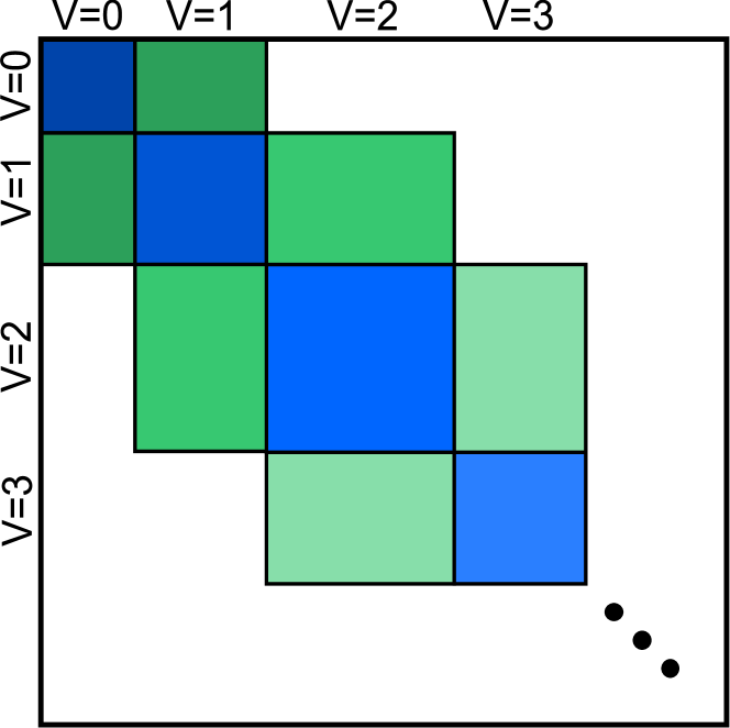
Figure 1: Illustration of the Hamilton matrix of a V-ordered occupation number basis. The blue parts contain the hopping terms inside a partition and the potential on the diagonal and the green parts contain the hopping terms between the partitions.

Note, that the hopping of a particle can only change the number $N_{\kappa}$ by one. Therefore, only neighboring sectors are coupled and the matrix has a tridiagonal block-structure.

3.1 Projection Step

We start out with a general projection based idea for solving an eigenvalue problem of a $2\times 2$ block matrix

$$A_{0}x=\begin{pmatrix}A&E\\ E^{\dagger}&B\\ \end{pmatrix}\begin{pmatrix}x_{1}\\ x_{2}\\ \end{pmatrix}=\lambda\begin{pmatrix}x_{1}\\ x_{2}\\ \end{pmatrix}\;.$$ (1)

The blocks correspond to some suitable partitions of the vector space under consideration. The sizes of the two partitions shall be denoted by $p_{1}$ and $p_{2}$, respectively. It is not necessary that the two partitions cover the entire vector space of the original problem.

We assume that $A$ and $E$ are ‘small’ compared to $B$, such that the lowest eigenvalue of $A_{0}$ is predominated by the corresponding eigenvalue of $A$ and the perturbation due to $E$ and $B$ can be included perturbatively. In order to quantify this idea, we will map the influence of the second partition into the first partition by a Schur transformation, similar to the projection technique [9, 10]. I.e. we multiply Eq. 1 from the left with the matrix

$$\begin{pmatrix}I&-EB^{-1}\\ 0&I\\ \end{pmatrix}$$

resulting in

$$\begin{pmatrix}S&0\\ E^{\dagger}&B\\ \end{pmatrix}\begin{pmatrix}x_{1}\\ x_{2}\\ \end{pmatrix}=\lambda\begin{pmatrix}I&-EB^{-1}\\ 0&I\\ \end{pmatrix}\begin{pmatrix}x_{1}\\ x_{2}\\ \end{pmatrix}\;,$$

with $S=A-EB^{-1}E^{\dagger}$ being the Schur-complement. The second line of the eigenvalue equation yields

$$x_{2}=-(B-\lambda)^{-1}E^{\dagger}x_{1}\;.$$ (2)

Inserting $x_{2}$ into the first line leads to

$$S_{\lambda}x_{1}:=(A-E(B-\lambda)^{-1}E^{\dagger})x_{1}=\lambda x_{1}\;.$$ (3)

Note that this equation is in principle exact, no approximations have been made so far. The original problem (Eq. 1) has thus been projected into the subspace of the first partition which is of smaller size, but at the prize of a non-linear eigenvalue problem. By the above procedure we obtain only those eigenvectors $x=(x_{1},x_{2})$ of the $2\times 2$ block matrix with non-vanishing $x_{1}$, i.e. those vectors which evolve perturbatively from those of $A$. There are additional eigenvectors of the form $x=(0,x_{2})$, which can, however, be omitted, since their eigenvalues are of order $O(V)$ instead of $O(t)$.

3.2 Solution of the non-linear eigenvalue problem

In the numerical projection technique, to be outlined below, the second partition will consist of a single sector. Hence $B$ will be the sub-matrix of the Hamiltonian corresponding to basis vectors of that particular sector and it will consist of a kinetic term and an interaction term, $B=\tilde{B}+B_{V}$, with $B_{V}=N_{\kappa}V\bf{I}$, where a $\bf{I}$ is a unit matrix. By virtue of this structure and the fact that $|V|\gg|t|$, the numerical solution of the non-linear problem can be simplified significantly. We can expand the inverse in powers of $B_{V}^{-1}$ or rather $(B_{V}-\lambda)^{-1}$. The latter step is justified, since the lowest eigenvalues are of order $t$ plus corrections of order $V^{-1}$, hence $B_{V}-\lambda=O(V)$. The expansion yields

$$\frac{1}{B-\lambda} = \frac{1}{B_{V}-\lambda+\tilde{B}}$$

$$= \frac{1}{B_{V}-\lambda}-\frac{1}{(B_{V}-\lambda)^{2}}\tilde{B}+\dots$$

$$= \sum_{\nu=0}^{\infty}\frac{1}{(B_{V}-\lambda)^{\nu+1}}(-\tilde{B})^{\nu}\;,$$

and the calculation of $S_{\lambda}$ becomes

$$S_{\lambda}=A+\sum_{\nu=0}^{\infty}(\lambda-B_{V})^{-(\nu+1)}\;E\;{\tilde{B}}^{\nu}\;E^{\dagger}\;.$$ (4)

Note that the expressions $(\lambda-B_{V})^{-(\nu+1)}$ are only numbers. For an iterative solution of the non-linear eigenvalue problem, $S_{\lambda}$ has to be computed repeatedly for different values of $\lambda$, but only the pre-factors $(\lambda-B_{V})^{-(\nu+1)}$ are modified. The matrices $E\tilde{B}^{\nu}E^{\dagger}$, however, are independent of $\lambda$. Therefore, they can be calculated once and stored, since they are in general of moderate size, as will be discussed later on.

This expansion can also be used in Eq. 2 in order to evaluate the second part of the eigenvector, i.e.

$$x_{2}=-(B-\lambda)^{-1}E^{\dagger}=-\sum_{\nu=0}^{\infty}(\lambda-B_{V})^{-(\nu+1)}\tilde{B}^{\nu}E^{\dagger}\;.$$

The non-linear eigenvalue problem can now be solved iteratively, by using an initial approximation for $\lambda$ to build $S_{\lambda}$, then solve the eigenvalue problem by suitable means and use the resulting eigenvalue as a new approximation for $\lambda$. Let $x_{\lambda}$ be the normalized eigenvector of $S_{\lambda}$ to the lowest eigenvalue $\mathcal{E}(\lambda)$. In the next recursion $\lambda^{\text{(new)}}=\mathcal{E}(\lambda)$ is used as new value for the parameter $\lambda$.

A more sophisticated approach to obtain an improved value for $\lambda$ is provided by the Newton-Raphson method. We are actually seeking the roots of $\Phi(\lambda)=\mathcal{E}(\lambda)-\lambda$. The Newton-Raphson approach yields

$$\lambda^{\text{(new)}}=\lambda-\frac{\Phi(\lambda)}{\Phi^{\prime}(\lambda)}=-\frac{1}{\mathcal{E}^{\prime}(\lambda)-1}\mathcal{E}(\lambda)+\frac{\mathcal{E}^{\prime}(\lambda)}{\mathcal{E}^{\prime}(\lambda)-1}\lambda\;.$$

The expression shows that this can be transformed to an equation of form $\lambda^{\text{(new)}}=\alpha\mathcal{E}(\lambda)+(1-\alpha)\lambda$ with

$$\alpha=-\frac{1}{\mathcal{E}^{\prime}(\lambda)-1}\;.$$

Note that in the simple iteration scheme $\alpha=1$. In order to calculate $\mathcal{E}^{\prime}(\lambda)$ we can use the Hellmann-Feynman theorem resulting in

$$\mathcal{E}^{\prime}(\lambda) =x_{\lambda}^{\dagger}S_{\lambda}^{\prime}x_{\lambda}\,.$$

The derivative of $S_{\lambda}$ (Eq. 3) with respect to $\lambda$ therefore reads

$$S_{\lambda}^{\prime}=-E(B-\lambda)^{-2}E^{\dagger}\;,$$ (5)

which, like Eq. 4, can be expressed in a Taylor expansion

$$\mathcal{E}^{\prime}(\lambda)=-\sum_{\nu=0}^{\infty}(\nu+1)(\lambda-B_{V})^{-(\nu+2)}x_{\lambda}^{\dagger}E\tilde{B}^{\nu}E^{\dagger}x_{\lambda}\;.$$ (6)

As before, the stored matrices $E\tilde{B}^{\nu}E^{\dagger}$ can be reused.

3.3 Iterative inclusion of higher sectors

Now we are in the position to describe the numerical projection technique. To begin with, we consider the following two partitions: the first partition may contain the lowest sectors $N_{\kappa}=0,1,\ldots,N^{\prime}$. The second partition consists of merely one sector, namely $N_{\kappa}=N^{\prime}+1$. The sizes of the partitions are $p_{1}$ and $p_{2}$, respectively. The projection step, discussed before, is used to combine the two partitions. This step can now be invoked repeatedly in order to include increasingly higher sectors.

1. We begin with the first partition, solve the eigenvalue problem for $A_{1}$ and determine the corresponding unitary matrix $V_{1}$ containing the corresponding $p_{1}$ eigenvectors.

2. The matrix for the first two partitions has the following block structure

   $$A_{2}=\begin{pmatrix}A_{1}&E_{1}\\ E_{1}^{\dagger}&B_{1}\\ \end{pmatrix}\;.$$

3. Next we perform a unitary transformation on $A_{2}$ provided by the unitary matrix $\text{diag}(V_{1},I)$ resulting in

   $$\tilde{A}_{2}:=\begin{pmatrix}D_{1}&V_{1}^{\dagger}E_{1}\\ E_{1}^{\dagger}V_{1}&B_{1}\\ \end{pmatrix}$$ (7)

   with $D_{1}:=V_{1}^{\dagger}A_{1}V_{1}$ being a $p_{1}$-dimensional diagonal matrix.

4. Now we solve the eigenvalue problem for $\tilde{A}_{2}\tilde{V}_{2}=\tilde{V}_{2}D_{2}$ as outlined in the previous section and construct the eigenvector matrix for the entire matrix $A_{2}$:

   $$V_{2}=\begin{pmatrix}V_{1}&\\ &I\\ \end{pmatrix}\tilde{V}_{2}\;,$$

   with $I$ being a identity matrix of appropriate size. As discussed before $\tilde{V}_{2}$ only contains the lowest $p_{1}$ eigenvectors. Consequently, $D_{2}$ is again a $p_{1}$-dimensional diagonal matrix.

5. Finally we include the blocks $E_{2}$ and $B_{2}$ of the next sector and perform again a unitary transformation with $\text{diag}(V_{2},I)$ as in Eq. 7  leading to

   $$\tilde{A}_{3}=\begin{pmatrix}D_{2}&V_{2}^{\dagger}E_{2}^{\phantom{{\dagger}}}\\ E_{2}^{\dagger}V_{2}^{\phantom{{\dagger}}}&B_{2}\\ \end{pmatrix}\;.$$

The recursion steps (d) and (e) are continued until the desired accuracy is reached.

3.4 Truncation of the first partition

The advantage of the numerical projection technique so far is the fact that (non-linear) eigenvalue problems have to be solved for matrices of a size given by the first partition $p_{1}$, which is obviously smaller then the original size.

→

→

…

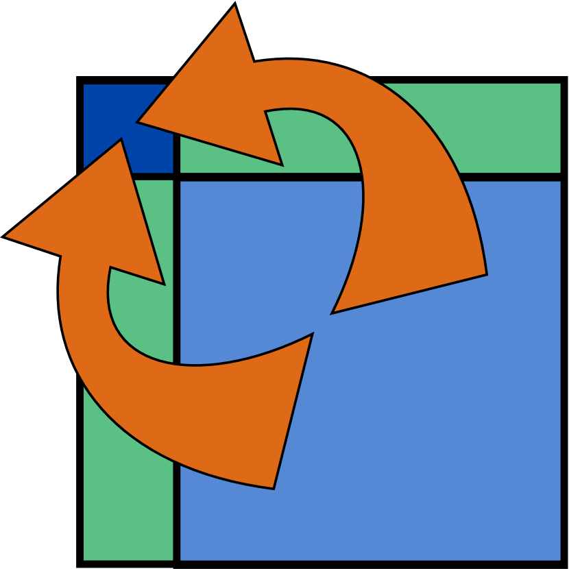
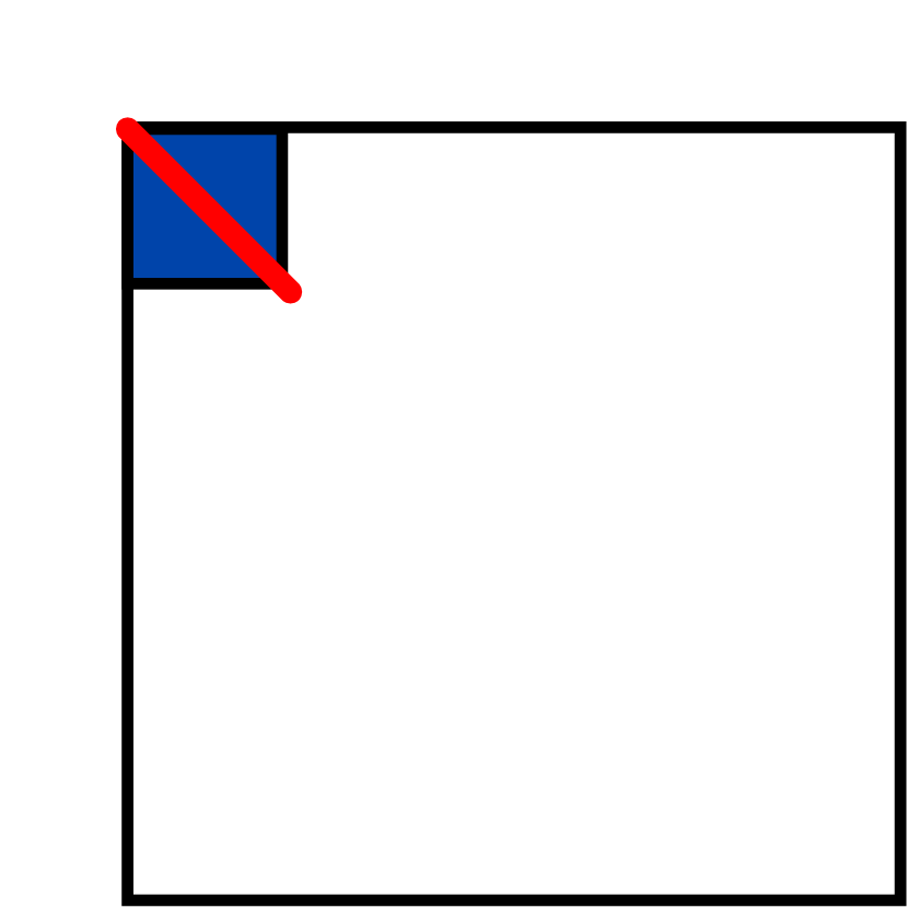
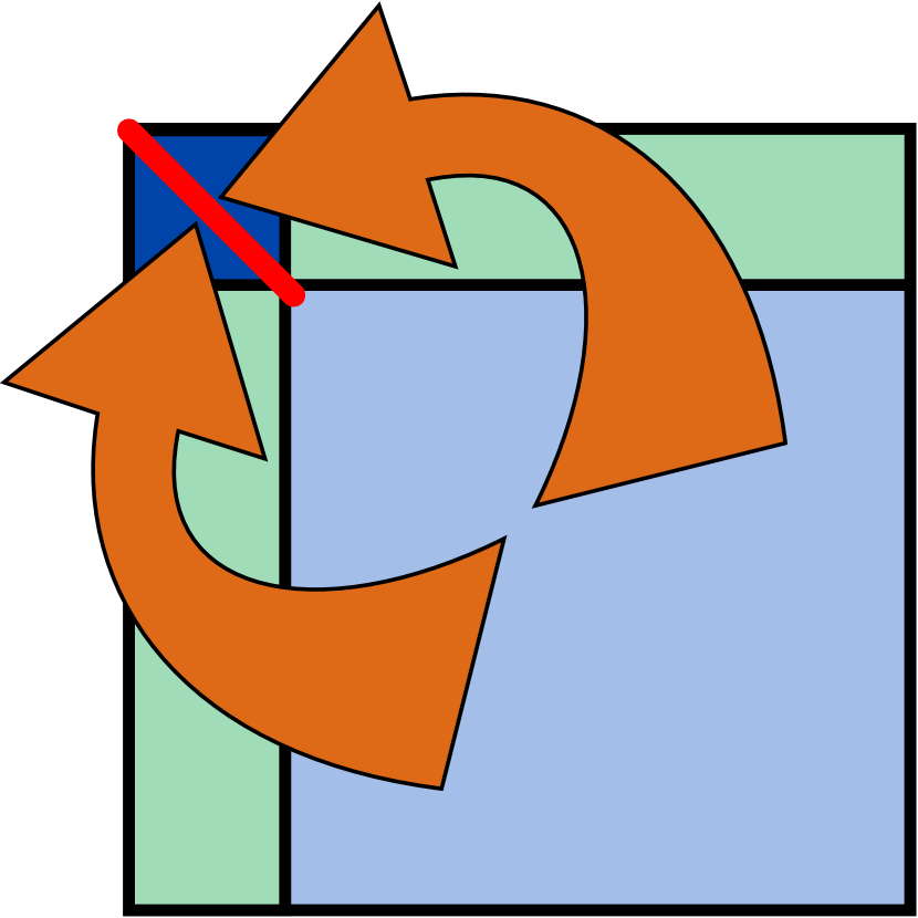
Figure 2: Truncation procedure for the scheme presented in the text. Each partition is consecutively projected onto the original effective matrix and diagonalized.

It may happen that the first partition, even if it covers merely the first sector, is still very large. This is the case in the Hubbard model, where already the lowest sector for $N_{\kappa}=0$ yields $p_{1}={L\choose N_{\uparrow}}{L-N_{\uparrow}\choose N_{\downarrow}}$, which at half-filling becomes $p_{1}={L\choose L/2}$. Next we will try and reduce the size of the first partition. Firstly, we can exploit translational invariance and solve the eigenvalue problem in the individual $k$-space sectors. We can furthermore restrict the number of vectors, which are retained in the first partition, based on some suitable criterion as to there importance for the lowest eigenvalue. We will use only the most obvious and simple criterion, namely to keep those vectors, which belong to the lowest eigenvalues $D_{2}$ of $A_{1}$. More sophisticated criteria as in DMRG are also conceivable.

We will use a predefined value $\tilde{p}_{1}\leq p_{1}$ for the truncation size of the first partition. That means, we solve the eigenvalue problem of $A_{1}$ of size $p_{1}\times p_{1}$ and retain only those $\tilde{p}_{1}$ eigenvectors in $V_{1}$ which correspond to the lowest eigenvalues. According to the recursion procedure, in the following recursion steps the diagonal matrices entering the left-upper block $D_{n}$ will all have the size $\tilde{p}_{1}$ and henceforth only (non-linear) eigenvalue problems of this size occur.

4 Numerical experiments

We begin with the spinless fermion model with periodic boundary condition (pbc) at half-filling. Due to the conservation of the total momentum $k$ only those basis vectors with the same $k$ need to be taken into account. For the spinless fermion model at half-filling the ground state is degenerate and has $k=\pm\frac{\pi}{2}$. We will therefore only take basis vectors into account, that have a total momentum $k=\pm\frac{\pi}{2}$. The selection of the total momentum leads to a significant reduction of the computational effort. On the one hand, the size $p_{1}$ of the initial partition is reduced roughly by $L$ and on the other hand it can be avoided that in the truncation step vectors are retained, that are irrelevant for the ground state of the original system.

To begin with, we choose as first partition the first sector with $N_{\kappa}=0$, which consists of merely 2 states with particles on every other site (charge density wave), i.e. $\tilde{p}_{1}=p_{1}=2$. These two vectors are the real valued linear combinations of the $\pm\frac{\pi}{2}$ basis vectors.

$L$	M	$t_{\text{NPT}}$ [s]	$t_{\text{AR}}$ [s]	$E_{\text{NPT}}$	$\left|\frac{E_{\text{NPT}}-E_{0}}{E_{0}}\right|$
16	12870	0.0	0.2	-1.57	0.007
18	48620	0.0	0.8	-1.76	0.010
20	184756	0.1	4.1	-1.95	0.012
22	705432	0.3	10.4	-2.14	0.014
24	2704156	0.6	87.1	-2.33	0.014

Table 1: Run-time and accuracy comparison between NPT ($t_{\text{NPT}}$, $E_{\text{NPT}}$) and traditional Arnoldi eigensolver (ARPACK, $t_{\text{AR}}$, $E_{0}$ ) for the spinless fermion model ($|V/t|=10$) at half-filling for different system sizes and pbc. The recursion was stopped at an absolute accuracy of $10^{-4}$. The matrices have size $M\times M$. All computations in this paper have been performed on a computer with Intel Core 2 Duo 3GHz, 2GB RAM.

Tab. 1 exhibits a comparison of the run time for various system sizes. It can be seen that NPT is significantly faster than the highly optimized ARPACK routine (Arnoldi implementation) for increasing system size. We observe that even for $10^{6}\times 10^{6}$-matrices the CPU time is less than 1 sec. and more than a hundred times faster than the highly optimized ARPACK code.

4.1 Dependence on the size of the initial partition

In Fig. 3 the upper curve (green squares) corresponds to the case that the initial partition consists of the first sector ($N_{\kappa}=0$) only, with $\tilde{p}_{1}=p_{1}=2$ and shows the dependence of the lowest eigenvalue on the maximum number of sectors, specified by $N_{\kappa}^{\text{max}}$, included in the recursion. We observe that the recursion rapidly levels off at a moderate relative accuracy of 1 percent. The reason is due to the fact, that the vectors that are omitted during the recursion procedure, are relevant for a higher accuracy.

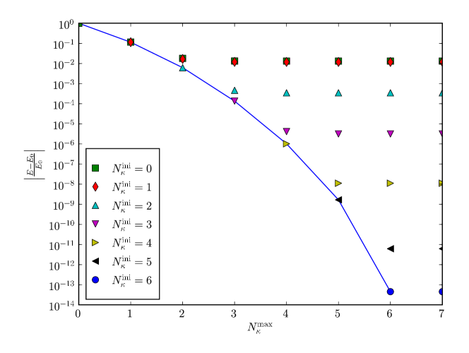
Figure 3: Convergence of the lowest eigenvalue with the largest sector ($N_{\kappa}^{\text{max}}$) included in the recursion, depending on the initial partition. In all cases, $\tilde{p}_{1}=2$ was used, i.e. the 2 lowest eigenvectors of the initial partition where kept. The blue solid line indicates the exact values corresponding the various subspaces (see text). The results are compared with the exact eigenvalue $E_{0}$ of the original matrix on a logarithmic scale. System parameters are $L=20,N=10,|V/t|=10$.

One way to increase the accuracy is to choose a greater initial partition upon including all sectors up to $N_{\kappa}^{\text{ini}}$, but still using a truncation size of the first partition $\tilde{p}_{1}=2$. The results are also depicted in Fig. 3. The turquoise upward triangles, e.g., depict the results for $N_{\kappa}^{\text{ini}}=2$, i.e. the initial partition contains sectors up to $N_{\kappa}=2$ and the subsequent recursions mix in $N_{\kappa}=3,\ldots,N_{\kappa}^{\text{max}}$. The relative accuracy increases by one order of magnitude but is still restricted. In all curves we observe that the result is converged when two more sectors are included beyond the ones present in the initial partition, which is obviously a consequence of the small truncation size $\tilde{p}_{1}=2$. The blue solid line indicates the result of the lowest eigenvalue obtained in the subspace spanned by the vectors of the sectors $N_{\kappa}=0,\ldots,N_{\kappa}^{\text{max}}$.

4.2 Dependence on the truncation size

So far we have seen that the accuracy is limited when the truncation size is restricted to 2, even if the size of the initial partition is increased and all sectors are iteratively included. One is therefore driven to study the dependence on the truncation size. To this end we consider one particular system ($L=20,N=10,|V/t|=10$) and choose as initial partition the lowest two sectors with $N_{\kappa}=0$ and $N_{\kappa}=1$. The size of the initial partition is $p_{1}=182$. In Tab. 2 the energies are listed for different truncation sizes $\tilde{p}_{1}$. In all cases NPT is iterated until an absolute accuracy of $\epsilon_{\lambda}=10^{-4}$ is reached. We observe a clear improvement as compared to the case $\tilde{p}_{1}=2$, although the accuracy is certainly limited by the fact, that only the first two sectors are included in the initial partition. We find that the accuracy achieved by using three sectors can never be reached.

$\tilde{p}_{1}$	$E_{\text{NPT}}$	$\left|\frac{E_{\text{NPT}}-E_{0}}{E_{0}}\right|$	$t_{\text{iters.}}[s]$
2	-1.9565	0.012	0.66
4	-1.9573	0.011	1.34
6	-1.9594	0.010	2.25
10	-1.9629	0.008	3.76
14	-1.9713	0.004	6.79
16	-1.9749	0.003	9.21
3 sectors	-1.9793	0.001
exact	-1.9800

Table 2: Dependence of the lowest eigenvalue on the truncation size $\tilde{p}_{1}$ for a system with $L=20$, $N=10$, $|V/t|=10$, $\epsilon_{\lambda}=10^{-4}$. Here, the initial partition consists of the first two sectors. In addition the exact lowest eigenvalue is given for a) the sub-matrix including the first three sectors and b) the original matrix.

5 Three-partition Projection

As discussed in the introduction, the central goal of the projection techniques is to describe the low-lying generic physics of the original quantum many-body system. We have seen, that NPT as opposed to standard projection techniques resulting in effective models, even yields quantitatively good agreement with the result of the the original model. If still higher accuracy is the ultimate goal, then one can do even better then what has been discussed so far. It is possible to include in each recursion step two sectors at a time with little more CPU effort. To this end we consider a matrix which has $3\times 3$ tridiagonal block structure, that results, if we add in each recursion (projection) step two additional sectors to the first partition. The matrix has the structure

$$\begin{pmatrix}A&E&0\\ E^{\dagger}&B&F\\ 0&F^{\dagger}&C\end{pmatrix}\;.$$

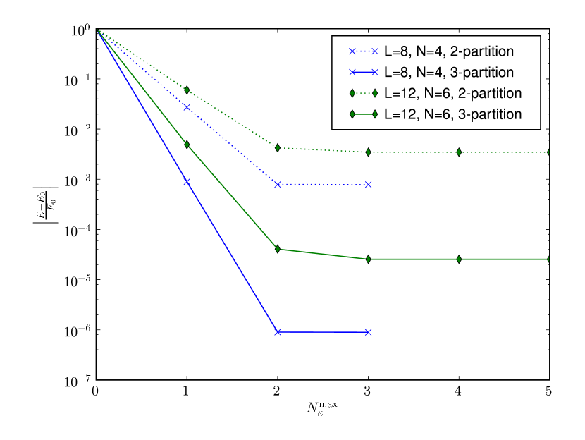
Figure 4: Comparison of the 2-partition and 3-partition approach for two different system sizes. The convergence of the relative uncertainty of the lowest eigenvalue is shown versus the maximum number of sectors included.

Here, an equivalent relation to Eq. 3 can be obtained:

$$\left(A-E\left(B-\lambda I-F(C-\lambda I)^{-1}F^{\dagger}\right)^{-1}E^{\dagger}\right)\vec{x}_{1}=\lambda x_{1}\;.$$

The contribution of the matrix $C$ shall be expanded up to the linear inverse term:

$$A-\lambda I- E\left(B-\lambda I\right)^{-1}E^{\dagger}$$

$$- E(B-\lambda I)^{-1}F(C-\lambda I)^{-1}F^{\dagger}(B-\lambda I)^{-1}E^{\dagger}$$

Again, the expression is expanded in terms of the kinetic part:

$$E(B-\lambda I)^{-1}F(C-\lambda I)^{-1}F^{\dagger}(B-\lambda I)^{-1}E^{\dagger}=\\ \sum_{\nu\mu\rho}\frac{1}{(B_{V}-\lambda)^{\nu+1}}\frac{1}{(B_{V}-\lambda)^{\mu+1}}\frac{1}{(C_{V}-\lambda)^{\rho+1}}\times\\ E(-\tilde{B})^{\nu}F(-\tilde{C})^{\rho}F^{\dagger}(-\tilde{B})^{\mu}E^{\dagger}\;.$$ (8)

Using this extension, the numerical result can be improved by orders of magnitude as is shown in Fig. 4. The results are for the spinless fermion model at strong coupling $|V/t|=10$ and half-filling. In both case the initial partition is given by the lowest sector without further truncation, i.e. $p_{1}=\tilde{p}_{1}=2$.

6 Results for the Hubbard model

Next we present some results for the Hubbard model.

system	model	$E_{\text{NPT}}$	$\left|\frac{E-E_{0}}{E_{0}}\right|$
$L=8$, $N_{\uparrow}=N_{\downarrow}=4$, $U=10$	Hubbard	-2.1767
	NPT ($\tilde{p}_{1}=20$)	-2.1526	0.0110
	Heisenberg	-2.2604	0.0385
$L=10$, $N_{\uparrow}=N_{\downarrow}=5$, $U=10$	Hubbard	-2.7037
	NPT ($\tilde{p}_{1}=26$)	-2.6572	0.0172
	Heisenberg	-2.8062	0.0379
$L=10$, $N_{\uparrow}=N_{\downarrow}=4$, $U=10$	Hubbard	-5.6698
	NPT ($\tilde{p}_{1}=80$)	-5.7303	0.0107
	tJ	-5.5282	0.0250
$L=10$, $N_{\uparrow}=N_{\downarrow}=5$, $U=5$	Hubbard	-4.9334
	NPT ($\tilde{p}_{1}=26$)	-4.6032	0.0669
	Heisenberg	-5.6123	0.1376

Table 3: Comparison of the lowest eigenvalue obtained by NPT with those of the Heisenberg or $tJ$-model and the exact result for the original Hubbard model. Periodic boundary conditions are assumed. Details of the NPT parameters are given in the text. One sectors were taken as initial partition ($N_{\kappa}^{\text{ini}}=1$).

Standard projection technique leads in the case of half-filling to the Heisenberg model and away from half-filling to the $tJ$-model [9]. These models correspond in NPT to the situation that the initial partition is the first sector with $N_{\kappa}=0$ (no double occupancies) and only the second sector is mixed in the projection step. On top of that, the non-linear eigenvalue problem is replaced by the linear one with $\lambda=0$ in Eq. 2. In Tab. 3 the lowest eigenvalues for different system sizes and particle numbers are given. In the half-filled case the NPT results are compared with the exact results for the corresponding Heisenberg model and away from half-filling with those of the $tJ$-model. In NPT we use the first sector ($N_{\kappa}=0$) as initial partition, restricted to $k=0$. For the truncation size in the projection steps we used $\tilde{p}_{1}=2$. The NPT recursion steps are stopped at an absolute accuracy $\varepsilon_{\lambda}=10^{-4}$.

We compare NPT results and those of the effective models with the exact lowest eigenvalue of the Hubbard model. We see that even in the strong coupling case ($|U/t|=10$), investigated here, NPT yields quantitatively better results than the effective models.

7 Conclusions

The numerical projection technique (NPT), presented in this paper, is a numerical generalization of standard projection technique, routinely used to derive effective models for qualitative description of the generic low-energy physics of strongly correlated systems. The standard projection technique corresponds to an approximate evaluation of second order perturbation theory in the inverse interaction parameter.

NPT on the one hand a systematic application of the projection techniques to any many-body Hamiltonian, irrespective of the complexity of the original model, also in cases where the analytic approach would lead to unmanageable effective models. On the other hand it is also applicable for moderate coupling parameters, where second order perturbation theory is not reliable enough.

We have demonstrated that NPT yields fairly accurate results with little CPU-effort as compared to state-of-the-art exact diagonalization. Furthermore, by solving the non-linear eigenvalue problem and including higher order terms the approach yields significantly better results than traditional projection technique.

References

- Lanczos [1950] C. Lanczos, An iteration method for the solution of the eigenvalue problem of linear differential and integral operators, Journal of Research of the National Bureau of Standards 45 (1950) 255–282.
- Parlett [1998] B. N. Parlett, The Symmetric Eigenvalue Problem, SIAM, Philadelphia, USA, 1998.
- Schollwöck [2005] U. Schollwöck, The density-matrix renormalization group, Rev. Mod. Phys. 77 (2005) 259–315.
- Cirac and Verstraete [2009] J. I. Cirac, F. Verstraete, Renormalization and tensor product states in spin chains and lattices, Journal of Physics A-Mathematical and Theoretical 42 (2009) 504004.
- Sénéchal et al. [2002] D. Sénéchal, D. Perez, D. Plouffe, Cluster perturbation theory for hubbard models, Phys. Rev. B 66 (2002) 075129.
- Potthoff [2003] M. Potthoff, Self-energy-functional approach: Analytical results and the mott-hubbard transition, The European Physical Journal B - Condensed Matter and Complex Systems 36 (2003) 335–348.
- von der Linden [1992] W. von der Linden, A quantum monte carlo approach to many-body physics, Physics Reports 220 (1992) 53 – 162.
- Evertz [2003] H. G. Evertz, The loop algorithm, Advances in Physics 52 (2003) 1.
- Fulde [1991] P. Fulde, Electron Correlations in Molecules and Solids, Springer series in solid-state sciences, Springer-Verlag, Berlin, Germany, 1991.
- Becker and Fulde [1988] K. W. Becker, P. Fulde, Ground-state energy of strongly correlated electronic systems, Zeitschrift für Physik B Condensed Matter 72 (1988) 423 – 427.
- M. et al. [2006] D. M., O. A. M., N. D. R., von der Linden W., Doping dependence of spin and orbital correlations in layered manganites, Phys. Rev. B 73 (2006) 104451.
- Imada et al. [1998] M. Imada, A. Fujimori, Y. Tokura, Metal-insulator transitions, Rev. Mod. Phys. 70 (1998) 1039–1263.
- Dagotto [1994] E. Dagotto, Correlated electrons in high-temperature superconductors, Rev. Mod. Phys. 66 (1994) 763–840.
- Dagotto et al. [2001] E. Dagotto, T. Hotta, A. Moreo, Colossal magnetoresistant materials: the key role of phase separation, Physics Reports 344 (2001) 1 – 153.
- Negele and Orland [1988] J. W. Negele, H. Orland, Quantum Many-Particle Systems, Westview Press, 1988.