The magnetic structure of Gd₂Ti₂O₇

Abstract

We attempt to solve the magnetic structure of the gadolinium analogue of ‘spin-ice’, using a mixture of experimental and theoretical assumptions. The eventual predictions are essentially consistent with both the Mössbauer and neutron measurements but are unrelated to previous proposals. We find two possible distinct states, one of which is coplanar and the other is fully three-dimensional. We predict that close to the initial transition the preferred state is coplanar but that at the lowest temperature the ground-state becomes fully three-dimensional. Unfortunately the energetics are consequently complicated. There is a dominant nearest-neighbour Heisenberg interaction but then a compromise solution for lifting the final degeneracy resulting from a competition between longer-range Heisenberg interactions and direct dipolar interactions on similar energy scales.

I Introduction

‘Spin-ice’ is now a well studied experimental system with interesting fundamental aspects1 . Originally the experimental investigation was undertaken to try to shed light on magnetic frustration. The lattice geometry is that of a pyrochlore: a three-dimensional network of corner-sharing tetrahedra. Although the triangle is geometrically frustrated a tetrahedron is much more so, culminating in an extensive degeneracy for the antiferromagnetic ground-state manifold for a Heisenberg bonded pyrochlore2 . ‘Spin-ice’ has the required geometry, but has a strong orbital and dipolar character that mean that the interactions are not Heisenberg-like and the ground-state is not even locally antiferromagnetic. This ‘failure’ has led to the current interest1 , but the original issue of pyrochlore magnetism remained. Other rare-earth atoms are much more Heisenberg-like, with gadolinium being archetypal. It is spherically symmetric as a consequence of having a half filled shell and, therefore, can be modeled as just a large fairly classical spin. The analogue ‘spin-ice’ material Gd₂Ti₂O₇3 has now been studied and the original issue of a Heisenberg pyrochlore has been investigated, subject to any residual dipolar issues.

The magnetic structure determination for Gd₂Ti₂O₇ and Gd₂Sn₂O₇ is currently a mess. The neutron scatterers predict bizarre states4 ; 5 , with different spins ordering with different moments and the system making no attempt to minimise the natural interactions. In contrast, the Mössbauer studies6 offer a simple picture of all sites equally ordered and the additional restriction that the moments lie in a particular plane perpendicular to a natural local crystallographic direction. In this article we try to rationalise both types of experiment and achieve a consistent magnetic structure.

The neutron scattering provides a magnetic state indexed by $\Big{(}\frac{1}{2},\frac{1}{2},\frac{1}{2}\Big{)}$. Since the system has an intrinsic four atoms per unit cell, this leads to thirty-two atoms per magnetic cell, rather more than is comfortable. We consequently start from the Mössbauer experiments which suggest that at low temperatures all moments are ordered with the restriction that they are ordered perpendicular to the natural local crystallographic direction. (Note that for spin-ice the spins are parallel to these local crystallographic directions, which corresponds to a reversal of the sign of the anisotropy interaction.) For a single tetrahedron this restriction is depicted in Fig.1.

Figure 1: Restriction of spins to a plane perpendicular to the local crystallographic directions pointing to the centre of the tetrahedron.

We stress that this restriction is not expected to be a dominant energetic restriction because the spin-orbit/dipolar aspects are likely to be very weak in comparison to the Heisenberg interactions. We are employing these constraints as experimental restrictions which only become fulfilled to extract some extra degeneracy from the choice of ground-state, once all stronger Heisenberg interactions have been optimised. Physically our arguments are consequently dangerous since slight avoidance of our constraints can provide energetic savings but be lost in the noise of the experiments!

We further enforce an energetic constraint that the total spin in each tetrahedron vanishes, which is suggested by the experiment but is not guaranteed by it. This then provides a tractable problem, which annotates the residual degeneracy of the Heisenberg model subject to the additional experimentally observed single-ion anisotropy. Note that this antiferromagnetic constraint is not applicable to spin-ice1 , where the orbital and dipolar complications provide a very non-Heisenberg interaction.

II Magnetic solutions

The solution of our constrained problem is much simplified using the normalised basis:

$${\bf\hat{S}}_{0}=\left[\frac{2}{3}\right]^{\frac{1}{2}}\left[{\bf\hat{x}}\cos x_{0}+{\bf\hat{y}}\cos y_{0}+{\bf\hat{z}}\cos z_{0}\right]$$ (1)

$${\bf\hat{S}}_{1}=\left[\frac{2}{3}\right]^{\frac{1}{2}}\left[{\bf\hat{x}}\cos x_{1}-{\bf\hat{y}}\cos y_{1}-{\bf\hat{z}}\cos z_{1}\right]$$ (2)

$${\bf\hat{S}}_{2}=\left[\frac{2}{3}\right]^{\frac{1}{2}}\left[-{\bf\hat{x}}\cos x_{2}+{\bf\hat{y}}\cos y_{2}-{\bf\hat{z}}\cos z_{2}\right]$$ (3)

$${\bf\hat{S}}_{3}=\left[\frac{2}{3}\right]^{\frac{1}{2}}\left[-{\bf\hat{x}}\cos x_{3}-{\bf\hat{y}}\cos y_{3}+{\bf\hat{z}}\cos z_{3}\right],$$ (4)

which is also subject to

$$x_{\alpha}=z_{\alpha}-\frac{2\pi}{3}\;\;\;\;\;\;\;\;y_{\alpha}=x_{\alpha}-\frac{2\pi}{3}\;\;\;\;\;\;\;\;z_{\alpha}=y_{\alpha}-\frac{2\pi}{3}$$ (5)

all modulo $2\pi$. This guarantees that the spins lie in the appropriate planes and also that they are normalised. The spins may also be decomposed as:

$${\bf\hat{S}}_{0}=\left[\frac{2{\bf\hat{x}}-{\bf\hat{y}}-{\bf\hat{z}}}{\surd 6}\right]\cos x_{0}+\left[\frac{{\bf\hat{y}}-{\bf\hat{z}}}{\surd 2}\right]\sin x_{0}$$ (6)

$${\bf\hat{S}}_{0}=\left[\frac{2{\bf\hat{y}}-{\bf\hat{z}}-{\bf\hat{x}}}{\surd 6}\right]\cos y_{0}+\left[\frac{{\bf\hat{z}}-{\bf\hat{x}}}{\surd 2}\right]\sin y_{0}$$ (7)

$${\bf\hat{S}}_{0}=\left[\frac{2{\bf\hat{z}}-{\bf\hat{x}}-{\bf\hat{y}}}{\surd 6}\right]\cos z_{0}+\left[\frac{{\bf\hat{x}}-{\bf\hat{y}}}{\surd 2}\right]\sin z_{0},$$ (8)

with analogues for the other three spins, which relates the chosen angles to the underlying Cartesian basis.

The solutions to the constraint (see Appendix)

$${\bf\hat{S}}_{0}+{\bf\hat{S}}_{1}+{\bf\hat{S}}_{2}+{\bf\hat{S}}_{3}={\bf 0}$$ (9)

may be characterised by the different ways of pairing the atoms. We have one style of solutions with all the angles equal

$$x_{0}=x_{1}=x_{2}=x_{3}\;\;\;\;\;\; y_{0}=y_{1}=y_{2}=y_{3}$$

$$\;\;\;\;\;\;z_{0}=z_{1}=z_{2}=z_{3}$$ (10)

and then three associated with pairs

$$x_{0}=x_{1}=-x_{2}=-x_{3}\;\;\;\;\;\; y_{0}=-y_{1}=y_{2}=-y_{3}$$

$$\;\;\;\;\;\;z_{0}=-z_{1}=-z_{2}=z_{3}$$ (11)

for the three choices of pairs of pairs.

The restrictions to the anisotropy plane and to antiferromagnetism severely constrain the permitted magnetic states. Once we have fixed one spin then there are (a maximum of) six permitted orientations for each spin in the local basis (a maximum of twenty-four globally). These states are generated by $x_{\alpha}\mapsto-x_{\alpha}$, $y_{\alpha}\mapsto-y_{\alpha}$ and $z_{\alpha}\mapsto-z_{\alpha}$, which are the only possibilities permitted by the Heisenberg model. The possible states are annotated in Fig.2. One can then generate possible

Figure 2: The six possible angles for a particular global spin configuration. This example is ${\bf S}_{0}$ and each spin configuration is described simultaneously by all three angles, $x_{0}$, $y_{0}$ and $z_{0}$.

global states from the initial spin, using one out of the four possible configurations in each subsequent tetrahedron, as depicted in Fig.3,

Figure 3: Possible spin configurations in an optimised tetrahedron, using the notation of Fig.2.

together with the analogues with $n\mapsto\bar{n}$ and independently the inverted tetrahedra.

The next step is to enumerate the possible global configurations. This proves quite difficult, however, so first we set the scene. For spin-ice the spin orientations are quite different, being controlled by ‘two in and two out’ for each tetrahedron. The spins are oriented towards the centres of the tetrahedra which induces less technical problems. All possible ground-states may be generated by propagation parallel to a Cartesian direction. One can place an arbitrary collection of spins in a particular plane of the geometry which places two spins in each participating tetrahedron. Any pairs that are either both in or both out propagate uniquely and each pair that are one in and one out provide two possible continuations. For each possible state we then propagate to the next plane generating an exponentially large number of possible ground-states. Note that this is not a solution to the spin-ice-like anisotropy projected Heisenberg model, which finds all spins in or all spins out and hence only two distinct ground-states because when one spin is chosen then all others are constrained.

For our model we follow a two stage process. Firstly we ignore the ‘bar’ and look only at the integer $n\in\{1,2,3\}$. For the special case of $z_{0}$=0 this distinction becomes moot anyway. Indeed, if we think a bit more physically, then we would not expect the spins to employ arbitrary directions and the special cases of $z_{0}\in\{0,\frac{2\pi}{3},\frac{4\pi}{3}\}$ and $z_{0}\in\{-\frac{\pi}{6},\frac{\pi}{2},\frac{\pi}{6}\}$ offer distinct extra symmetries with both involving only twelve global spin orientations. The first provides a restriction to only three local orientations and the second finds commonality between distinct sublattice configurations leading to the orientations:

$$\{\frac{\pm{\bf\hat{y}}\pm{\bf\hat{z}}}{\surd 2},\frac{\pm{\bf\hat{z}}\pm{\bf\hat{x}}}{\surd 2},\frac{\pm{\bf\hat{x}}\pm{\bf\hat{y}}}{\surd 2}\}.$$ (12)

This second option is probably the best candidate for the experimental systems. By employing propagation along one of the Cartesian directions, we can use a similar argument to the previous to investigate the degeneracy. We focus on a plane perpendicular to the $z$-direction for which Fig.3 provides the restrictions that $1$ and $2$ may not be neighbours in the plane but pairs of $1$ and $2$ may propagate to the next plane using either $1$ or $2$ for the next pair. This provides a large but seemingly not exponential degeneracy, since as well as the new configurations from the choices of $1$ and $2$, there is also an associated loss from discounting states where $1$ and $2$ are neighbours in the next plane. The inclusion of the bar further complicates matters.

We now consider the scattering experiments and include the idea that the scattering can be indexed using $\Big{(}\frac{1}{2},\frac{1}{2},\frac{1}{2}\Big{)}$. At the simplest level this restriction amounts to choosing the sixteen spins of Fig.4, subject to the previous restrictions of Fig.3, combined

Figure 4: Distinct atoms in the magnetic unit cell. $\bar{n}$ are in the reverse direction to $n$.

with the constraint that the ‘barred’ spins are reversed in orientation. In our modeling, this restriction to having reversed spins is also a strong constraint. The easiest way to enforce it is to restrict attention to $z_{0}$=$\frac{\pi}{2}$ and then in Fig.2 the two spins $n$ and $\bar{n}$ are actually in opposite physical directions. The previous problem of annotating permissible configurations in terms of the states $n$ now provides an elementary solution: we find four styles. Firstly, pure solutions where each site has the same $n$. Secondly, alternating solutions where in a particular direction planes alternate between two distinct values of $n$. Thirdly, tetrahedral solutions with alternating tetrahedra alternating between two distinct values of $n$. Fourthly, period-four solutions where one plane in four has a distinct value of $n$. Fig.5 shows the only two examples which are are consistent with $\Big{(}\frac{1}{2},\frac{1}{2},\frac{1}{2}\Big{)}$.

Figure 5: Possible spin configurations for the case $z_{0}$=$\frac{\pi}{2}$.

A second set of solutions may be obtained from $z_{0}$=-$\frac{\pi}{6}$ where now the pairs $\{1,\bar{2}\}$ $\{2,\bar{3}\}$ and $\{3,\bar{1}\}$ correspond to reversed spins. The permitted solutions are depicted in Fig.6,

Figure 6: Possible spin configurations for the case $z_{0}$=-$\frac{\pi}{6}$.

and there are only four physically distinct styles. Clearly by employing symmetry there are a mass of rotation and translationally associated analogues to the depicted states. In total, however, there appear to be only six styles of solutions. Careful investigation of these states demonstrate that in fact there are only two classes unrelated by symmetry, which we can choose to be the $z_{0}$=$\frac{\pi}{2}$ states of Fig.5. The first is coplanar and the second fully three-dimensional.

III Experimental and theoretical issues

There is one critical final piece in the puzzle: the form-factors of the magnetic Bragg spots. The internal structure of our proposed states can be probed by measuring the relative intensities of the different magnetic Bragg spots. In our notation the strengths of the nearest Bragg spots to the origin are directly related to the magnetic moments on each of the four underlying sublattices:

$${\bf B}_{0}={\bf S}_{0}+{\bf S}_{1}+{\bf S}_{2}+{\bf S}_{3}\;\;\;\;\;\;\;{\bf B}_{1}={\bf S}_{4}+{\bf S}_{5}+{\bf S}_{6}+{\bf S}_{7}$$ (13)

$${\bf B}_{2}={\bf S}_{8}+{\bf S}_{9}+{\bf S}_{10}+{\bf S}_{11}\;\;\;\;\;\;\;{\bf B}_{3}={\bf S}_{12}+{\bf S}_{13}+{\bf S}_{14}+{\bf S}_{15}.$$

In all of our states these quantities vanish!

The actual $\Big{(}\frac{1}{2},\frac{1}{2},\frac{1}{2}\Big{)}$ Bragg spot, and its symmetrically related neighbours, correspond to decomposing the lattice into alternating planes of Kagomé connectivity and sparse triangular planes, keeping the phase within such a plane uniform and alternating the phase between neighbouring equivalent geometries. Interestingly, our antiferromagnetic ansatz directly controls this character. The Kagomé planes may be decomposed into two inversion related sets of triangles, as depicted in Fig.7. One set (a) corresponds to a set of triangular faces

Figure 7: Kagomé plane decomposed into the two inversion related triangles. The (a) denote atoms that complete tetrahedra above and the (b) denote atoms that complete tetrahedra below.

of tetrahedra which are completed above the plane, and the other (b) form a set of corresponding tetrahedra which are completed below the plane. These completing atoms form the neighbouring sparse triangular planes. The imposed constraint that each tetrahedron has zero total spin then enforces that the total spin in a Kagomé plane is antiparallel to both neighbouring triangular planes. The phase relationship that ‘neighbouring’ triangular planes should be antiparallel then requires that the total spin in each Kagomé plane must vanish. Consequently the associated Bragg spots must also vanish. Physically the argument only depends on the nearest-neighbour Heisenberg interactions: solving each tertrahedron gives the requirement that that tetrahedron should have vanishing total spin. The Kagomé argument of Fig.7 requires that the total spin of each neighbouring plane along the (1,1,1) direction (or analogues) must be antiparallel. Since the relevant Bragg spots add every second plane with an alternating sign, the appearance of such a Bragg spot is inconsistent with the nearest-neighbour Heisenberg interaction. We have also imposed the additional constraint that our solutions have the observed magnetic periodicity which requires that the total-spin of each plane vanishes.

This argument provides a second important physical consequence. In terms of the original four atoms per unit cell of the underlying pyrochlore structure, the triangular lattices between Kagomé planes provide each of the four sublattices as the orientation of the Kagomé planes is varied. This fact tells us that the total spin of each sublattice independently vanishes. Although we have developed our argument employing spin anisotropy and experimental periodicity, our chosen states automatically minimise spin interactions that we did not impose. To see this we next analyse third-nearest neighbour Heisenberg interactions, which in this case are expected to be stronger than the second-nearest neighbour interactions due to the nature of relavent interaction pathways. We find that the third-nearest neighbour interactions are restricted to connect atoms on the same original sublattice. There are twelve such third-neighbours to each spin and they come in two classes. Firstly, there are six neighbours with a magnetic gadolinium atom lying exactly in the middle between them. Secondly, the other six neighbours have a non-magnetic titanium atom lying between them. The gadolinium chains form the original face-centre-cubic lattice but with bonds omitted between neighbouring atoms lying in planes perpendicular to the appropriate (1,1,1) direction. In our notation, this interaction is optimised by maximising the total spin of the four atoms on the same sublattice rather than minimising it. The chains of alternating gadolinium and titanium atoms yield the sparse triangular lattices in-between the Kagomé planes. Although our vanishing total spin on these planes is a low energy state for these third neighbour interactions, it is only the ground-state of the triangular lattice when there are additional longer-neighbour interactions also present.

We now embark upon a low level analysis of the plausible energetic interactions responsible for our proposed states. There is a sizable literature which we do not do justice to. The most relevant mean-field analysis of the Heisenberg interactions is not compatible with the actual interactions in this system7 , using physical distance instead of active pathways to choose the relevant interactions. The dipolar investigations are more relevant3 ; 8 and indicate that the lowest energy solution should be a q=0 state8 although (q,q,q) states should also be low energy states3 and therefore competitive. We employ much simpler arguments to try to get to grips with the most likely physical explanation for the observed experimental states.

The actual additional Heisenberg interactions probably stem from pathways across titanium atoms, since the hopping matrix elements are so much larger. The cage of atoms depicted in Fig.8

Figure 8: Cage of gadolinium atoms surrounding a tetrahedron of titanium atoms.

are all expected to develop Heisenberg interactions of various strengths between the members, although the bonds between members of the same sublattice should be largest. We employ two new matrix elements for the additional Heisenberg interactions across the hexagons depicted in Fig.8: $\lambda$ for diametric and $\kappa\lambda$ for the remaining two interactions. The structure factor is then controlled by the matrix:

$$\Gamma_{\bf k}=\left[\begin{matrix}\lambda\left(4xyz-1\right)&X+2\lambda\kappa xc_{1}&Y+2\lambda\kappa yc_{2}&Z+2\lambda\kappa zc_{3}\\ X+2\lambda\kappa xc_{1}&\lambda\left(4xYZ-1\right)&z+2\lambda\kappa Zc_{3}&y+2\lambda\kappa Yc_{2}\\ Y+2\lambda\kappa yc_{2}&z+2\lambda\kappa Zc_{3}&\lambda\left(4XyZ-1\right)&x+2\lambda\kappa Xc_{1}\\ Z+2\lambda\kappa zc_{3}&y+2\lambda\kappa Yc_{2}&x+2\lambda\kappa Xc_{1}&\lambda\left(4XYz-1\right)\\ \end{matrix}\right]$$ (14)

with,

$$x=\cos\frac{k_{y}-k_{z}}{2}\;\;y=\cos\frac{k_{z}-k_{x}}{2}\;\;z=\cos\frac{k_{x}-k_{y}}{2}$$ (15)

$$X=\cos\frac{k_{y}+k_{z}}{2}\;\;Y=\cos\frac{k_{z}+k_{x}}{2}\;\;Z=\cos\frac{k_{x}+k_{y}}{2}$$ (16)

$$c_{1}=\cos k_{x}\;\;\;c_{2}=\cos k_{y}\;\;\;c_{3}=\cos k_{z}$$ (17)

as the associated parameterisation. In the absence of the perturbations this structure factor has two degenerate bands at $\Gamma=-1$ which control the spin degeneracy. We treat the additional perturbations as small and solve for the lifting of this degeneracy in the two degenerate bands. Employing the parameter $\epsilon$ to control the eigenvalues:

$$\Gamma=-1-\lambda-2\lambda\epsilon,$$ (18)

we find that the perturbed structure factor satisfies:

$$(1-a_{2})\epsilon^{2}-2\big{(}a_{2}[1+4\kappa]+3a_{2}^{2}-a_{1}[3a_{1}+a_{3}][1+\kappa]\big{)}\epsilon+3a_{2}^{2}[4\kappa^{2}-1]-a_{3}[a_{3}+2a_{1}][1+\kappa]^{2}+9a_{1}^{2}a_{2}[1-\kappa^{2}]+6a_{1}a_{2}a_{3}[1+\kappa]-9a_{2}^{3}=0$$ (19)

in terms of

$$a_{1}=\frac{c_{1}+c_{2}+c_{3}}{3}\;\;\;a_{2}=\frac{c_{2}c_{3}+c_{3}c_{1}+c_{1}c_{2}}{3}\;\;\;a_{3}=c_{1}c_{2}c_{3}.$$ (20)

This can then be minimised to predict the likely positions of the Bragg spots stemming from these physical interactions. Although the observed experimental Bragg scattering is at low energy, there is always a lower energy solution that finds a spiral parallel to one of the Cartesian axes. The ground-state as a function of $\kappa$ involves a solution of the form:

$$c_{1}=c_{2}=-\cos\theta\;\;\;c_{3}=1.$$ (21)

This spiral starts out with $\theta=\frac{\pi}{3}$ when $\kappa=0$ and ends up at the experimental $\theta=\frac{\pi}{2}$ with the unphysical value of $\kappa=1$, as depicted is in Fig.9.

Figure 9: Angle of the spiral measured in units of $\pi$.

The energy of this ground-state is compared to that of the experimental solutions and the zone-centre solution in Fig.10.

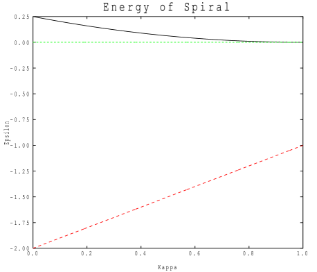
Figure 10: Energies of various states, ground-state (bold), experimentally observed state (dotted) and zone-centre (dashed).

It is clear that the second-neighbour Heisenberg interactions are not sufficient to describe the physics, and that the zone-centre state has a very poor energy. It therefore appears necessary to resort to the dipolar interactions to energetically explain the observed phases.

Dipolar interactions take the generic form

$$\hat{H}=\frac{{\bf S}_{\alpha}.{\bf S}_{\beta}-3{\bf S}_{\alpha}.{\bf\hat{r}}_{\alpha\beta}{\bf\hat{r}}_{\alpha\beta}.{\bf S}_{\beta}}{\mid{\bf r}_{\alpha\beta}\mid^{3}}$$ (22)

where ${\bf r}_{\alpha\beta}\equiv{\bf r}_{\alpha}-{\bf r}_{\beta}$ is the vector connecting the two interacting spins. This interaction is mathematically taxing because it is both long-range and it relates the spin orientation to the lattice directions which breaks spin isotropy. We will extract the initial isotropic Heisenberg interactions which renormalise the existing exchange-based interactions and focus only on the second term. This second term we further restrict to nearest-neighbours:

$$\hat{H}=-3\sum_{\alpha>\beta}{\bf S}_{\alpha}.{\bf\hat{r}}_{\alpha\beta}{\bf\hat{r}}_{\alpha\beta}.{\bf S}_{\beta}.$$ (23)

It is elementary to solve this rescaled dipolar interaction on a single tetrahedron and we find five styles of solution at energies: $\{-\frac{3}{2}(1+\surd 17),-3,3,\frac{3}{2}(\surd 17-1),12\}$. The ground-state has 86.4% of its moments parallel and is consequently a high energy state if the nearest-neighbour Heisenberg interaction dominates. The next state is triply degenerate and as it has zero total-spin it is compatible with the Heisenberg interaction. The third state is doubly degenerate and also has zero total-spin. The fourth state is not compatible as it has 13.6% of its moments parallel. Finally the fifth state also has zero total-spin. The three compatible styles of states are depicted in Fig.11

Figure 11: Total-spin zero eigenstates of the short-range dipolar model, in order of energy.

and the crucial observation is that the two low energy states involve spins which are perpendicular to the natural crystallographic directions (i.e. the spins are in the planes indicated by the Mössbauer experiments).

The planar spin restrictions deduced from the Mössbauer experiments can be derived from the nearest-neighbour dipolar interactions subjected to dominant nearest-neighbour Heisenberg interactions. Enforcing equal length spins and including the Heisenberg constraints, Eq.(9), we may rewrite the dipolar interactions, Eq.(23), as

$$\hat{H}=\frac{3}{4}\big{[}(S_{0}^{x}+S_{0}^{y}+S_{0}^{z})^{2}+(S_{1}^{x}-S_{1}^{y}-S_{1}^{z})^{2}\;\;\;\;\;\;$$

$$+(-S_{2}^{x}+S_{2}^{y}-S_{2}^{z})^{2}+(-S_{3}^{x}-S_{3}^{y}+S_{3}^{z})^{2}\big{]}$$

$$+\frac{3}{8}\big{[}(S_{0}^{x}+S_{1}^{x}-S_{2}^{x}-S_{3}^{x})^{2}\;\;\;\;\;\;\;\;\;\;\;\;\;\;\;\;\;\;\;\;\;\;\;\;$$

$$+(S_{0}^{y}-S_{1}^{y}+S_{2}^{y}-S_{3}^{y})^{2}\;\;\;\;\;\;\;\;\;\;\;\;\;\;\;\;\;\;\;\;$$

$$+(S_{0}^{z}-S_{1}^{z}-S_{2}^{z}+S_{3}^{z})^{2}\big{]}\;.\;\;\;\;\;\;\;\;\;\;\;\;\;$$ (24)

This is clearly minimised by zeroing each of the seven quadratics, which is consistent and indeed uniquely specifies the three states shown later in Fig. 15. In particular we note that the first four quadratics may be represented by

$$\left[{\bf S}_{0}.(1,1,1)\right)]^{2}\;\;\;\;\;\;\;\;\;\;\left[{\bf S}_{1}.(1,-1,-1)\right]^{2}\;\;\;$$

$$\left[{\bf S}_{2}.(-1,1,-1)\right]^{2}\;\;\;\;\;\;\;\;\left[{\bf S}_{3}.(-1,-1,1)\right]^{2}\;.$$ (25)

Orienting the four spins perpendicular to their local crystallographic directions therefore partially minimises the local dipolar energy.

One might now conclude that the problem is solved. We have a dominant nearest-neighbour Heisenberg interaction with a weaker dipolar interaction which stabilises the observed experimental states, but this is not the case. There is a clear solution to the problem of dominant nearest-neighbour Heisenberg and weak nearest-neighbour dipolar forces and it is not the experimentally observed state. Instead all that is required is to repeat the spiral solution of Fig.11 in all directions to provide a compatible solution that has ${\bf k}={\bf 0}$8 . The only way to now rationalise the experiments is to assume that there is a competition between the dipolar forces and the longer-range Heisenberg interactions. The energy of the Heisenberg interactions at ${\bf k}={\bf 0}$ is $\epsilon$=-2+$\kappa$ which is much worse than $\epsilon$=0 for the experimental solutions. We can then argue that dipolar interactions are not strong enough to overcome this energy but are strong enough to select the observed ground-state over the weak preference by the second and third-neighbour Heisenberg interactions.

The next task is to assess the dipolar energies in the language that we have used to describe our solutions. The dipolar states which do not respect zero total-spin can be split into pieces which are parallel and perpendicular to the natural crystallographic directions. We find the ‘two in and two out’ state of spin-ice parallel to the crystallographic directions and a saturated ferromagnetic state parallel to a Cartesian direction. These states are consequently totally irrelevant. The high energy state is also restricted to the crystallographic directions and hence we are restricted to the first two states depicted in Fig.11. Careful calculation of the dipolar energies of the six bonds in a tetrahedron then yields

$$D=\cos x_{0}\cos x_{1}+\cos x_{2}\cos x_{3}\;\;$$

$$+\cos y_{0}\cos y_{2}+\cos y_{1}\cos y_{3}\;\;$$ (26)

$$+\cos z_{0}\cos z_{3}+\cos z_{1}\cos z_{2}\;\;$$

and when we further incorporate our solutions to nearest-neighbour Heisenberg interactions we find

$$D_{0}=3\;\;\;\;\;\;\;\;\;\;\;D_{1}=3\cos(2x_{\alpha})$$

$$D_{2}=3\cos(2y_{\alpha})\;\;\;D_{3}=3\cos(2z_{\alpha})$$ (27)

for each of the configurations depicted in the columns of Fig.3 (where $\alpha\in\{0,1,2,3\}$ is any of the spins). Minimising these energies clearly leads to two of the general dipolar eigenstates (shown in Fig. 11). However, it also highlights the solutions $z_{0}\in\{\frac{\pi}{2},\pm\frac{\pi}{6}\}$ that we previously required, in order to be consistent with $\Big{(}\frac{1}{2},\frac{1}{2},\frac{1}{2}\Big{)}$. We can now, therefore, choose the value of $z_{0}$ to optimise the dipolar interactions rather than to fit the experiments.

The final task in this section is to analyse the solutions that we previously found for their dipolar content. The first half of the states depicted in both Fig.5 and Fig.6 involve half of the tetrahedra being in the dipolar ground-state and the other half being in the high energy state. The second set of states also involve half of the tetrahedra being in the dipolar ground-state but the other half are not in eigenstates of the dipolar interaction at all, but instead are superimposed three-quarters the high energy state and a quarter the ground-state. Consequently the more exotic states are actually lower in dipolar energy and therefore expected to be favoured at low temperatures.

One crucial observation is that for our coplanar states the dipolar interactions are energetically consistent with the nearest-neighbour Heisenberg interactions while for the non-coplanar states they are not. Although the spin state in each tetrahedron is not always the ground-state, for the coplanar state it is always a local eigenstate. For the non-coplanar states, however, half of the tetrahedra have states which are not local eigenstates. Consequently the system would be expected to relax slightly to improve the dipolar energy a little at the expense of the nearest-neighbour Heisenberg energy. This provides a physical mechanism for the magnetic Bragg spots closest to the origin to appear!

IV State characterisation

Our final task is to try to characterise our different solutions so that they might be separated both theoretically and experimentally. The joint issues of quantum fluctuations, thermal disorder and static disorder will all lift degeneracy and prefer particular states. Quantum fluctuations prefer collinear states9 , which allows more coherent fluctuations. Static disorder, however, prefers non-collinear states10 , which allow static distortions in perpendicular directions to the disorder field. Thermal fluctuations prefer the highest density of states at low energies, to optimise entropy, so called ‘order from disorder’11 . This tends to offer similar states to those stabilised by quantum fluctuations. Our states come in two classes, the first half of each set of states in Fig.5 and Fig.6 are coplanar and the second half involve fully three-dimensional spin orientations (although admittedly only eight of the twelve conceivable). We might anticipate the coplanar solutions to be stable at low temperature, on quantum fluctuation grounds, but alternatively we might expect the non-coplanar states on dipolar grounds. It is natural to associate the observed transition in Gd₂Ti₂O₇ as a transition between the two possible states, but we have no overwhelming experimental insights that provide clues as to which order of states one might like to pick.

The experiments do provide an important anomaly. Although in the first investigation4 the Bragg spots closest to the origin were seen to vanish, the more careful investigation5 found small intensities which were attributed to the low temperature phase. As we have pointed out, such spots are inconsistent with the nearest-neighbour Heisenberg model. There are various options. Firstly, the observed scattering might be diffuse and associated with disorder. It is known that diffuse scattering is much larger than usual in non-collinear magnets12 . Secondly, the magnetic state is expected to break the cubic symmetry and hence there is no longer a requirement that the Heisenberg interaction is perfect. Thirdly, the scattering might be nuclear in origin and hence be associated with a tiny structural distortion (although this appears physically quite unlikely). The dipolar forces argument suggests that coplanar states yield no Bragg intensity but that non-coplanar states yield a small one; this is the only clue we have to offer.

The actual spin arrangements are quite complicated and hence are difficult to depict. We have taken half of the magnetic cell and pictured the coplanar and non-coplanar states respectively in Fig.12 and Fig.13.

Figure 12: Coplanar spin arrangement.

Figure 13: Non-coplanar spin arrangement.

The complete spin arrangements are constructed from these by A-B ordering a full cubic super-lattice using the depicted cell and its spin inverse as the decoration for the super-lattice.

V Paradox

We now arrive at a theoretical paradox: our calculations are inconsistent with the current theoretical literature! We have found a complete set of solutions to our assumptions and the local dipolar energy is much worse than the ${\bf q}={\bf 0}$ solution that is expected from the ‘order from disorder’ calculations8 . The entire ethos behind that calculation was the lifting of a degeneracy that remained when the dipolar interaction was included, essentially exactly in the classical limit at zero temperature. In our calculations we ought to have found a solution that was degenerate with the ${\bf q}={\bf 0}$ solution.

There are various possible resolutions. Firstly, we have restricted our calculations to states which are orthogonal to the natural crystal directions and this eliminates two additional zero total-spin states from our optimisation. One is the state with spins pointing to the centre of the cube and the other is the state depicted in Fig.14.

Figure 14: Possible spin configuration ignored so far.

Both of these states are of much higher energy than the ground-state. Use of these additional states, therefore, cannot lift us to the energy of the ${\bf q}={\bf 0}$ solution. Indeed, we can exactly solve the problem of dominant nearest-neighbour Heisenberg and local dipolar interactions: we are restricted to the states depicted in Fig.15.

Figure 15: Local dipolar ground-states when total-spin of tetrahedron vanishes.

These states, which are in the perpendicular subspace, constitute only three of the possible configurations in Fig.3. For the case $z_{0}=0$ they are the three configurations with $\{n,n,\bar{n},\bar{n}\}$, and we can only construct q=0 solutions from these configurations Secondly, we have only considered the local dipolar interaction and the longer-range contributions could overturn our argument. Although the dipolar interaction is long-range, the divergence is irrelevant and we do not anticipate issues here. Thirdly there might be a loop-hole in the previous theoretical arguments. The previous calculations for the Heisenberg and dipolar interactions combined3 calculated the effective structure factor for the classical magnetic problem, but they did not proceed on to provide an actual magnetic solution. It was presumed that an appropriate magnetic solution would exist. Unfortunately, this is not guaranteed. For classical magnetism there are additional constraints: the magnitude of the spin of each atom on each sublattice must independently be normalised13 . For Heisenberg-like exchange models there is always an elementary spiral (in all bar the Ising model) that will provide a solution. In this dipolar problem, however, one needs to make a multiple-q state involving all four appropriate q’s, and there are simply not enough spin dimensions to satisfy all the constraints. It would appear that solving the dipolar problem is harder than first imagined.

VI More experimental and theoretical issues

In this section we range across the main experiments that have been performed on Gd₂Ti₂O₇ and comment on their relationship to our and previous proposals in the literature. We start out with local probes: Mössbauer and muon spin rotation.

The Mössbauer experiments6 offer the assertion that the spins are all the same length and that they are oriented perpendicular to the local crystallographic directions, assumptions that we employed in our modeling. More careful reading exhibits the possibility of two magnetic moments not both in the preferred planes, but only in the initial intermediate temperature phase. An additional degree of freedom always provides a better fit; the improvement is not significant. The second magnetic moment is also much too large to agree with the states proposed by the neutron scatterers. The low temperature phase does not appear to accept a phase with two different moments.

The muon spin-rotation experiment14 offers two clues. Firstly the muon sees two magnetic sites with slightly different fields and a non-magnetic site (or a parallel spin). Secondly there is a sizable relaxation even at very low temperatures. Due to the lack of knowledge about where the muon sits (probably in a low symmetry position close to one of the oxygens) the magnetic information is not easily usable. The relaxation tells us that there are active low energy excitations disturbing the spins even at the lowest temperatures. Also present in this investigation is some specific heat data, which is most instructive. The majority of the entropy is dissipated above the magnetic transitions and the entropy goes to zero at zero temperature with a power law. There is no residual degeneracy at zero temperature and the low temperature behaviour is well represented by some low energy excitations (surprisingly low energy perhaps). It is therefore, not possible that a macroscopic fraction of the spins are locally disordered in the vicinity of the magnetic phase transition. Any disorder must be highly correlated and associated with minimal entropy, viz a few well defined excitations.

There are some very interesting neutron spin-echo measurements15 ; 16 . This pretty experiment gives direct access to the time dependence of the magnetic correlations. The long-time limit clearly shows the expected long-range order. The temporal decay of the measurement exhibits the time-scale on which the fluctuations disorder the initial ‘snapshot’ of the spin correlations. Thermal fluctuations are expected to decay at low temperature and so the measurement flattens at low temperature16 . The most intriguing aspect is the fact that on observable time-scales the signal does not saturate, but appears to converge to three-quarters! This is taken to mean that a quarter of the spins are fluctuating, but from the specific heat data, they would have to be doing this coherently. It is not clear from the papers how this normalisation is accomplished, because naively one takes a very low temperature and zero field to normalise the data, assuming that the system has no residual dynamic fluctuations there. If this result is correct, then it is certainly interesting.

Finally we come to the elastic neutron scattering4 ; 5 , with the proposal of states with spins of different average length. Although it is stated that the neutron scattering promotes only these states, the current paper clearly shows that states exist which are consistent with the elastic neutron scattering and the Mössbauer restrictions that the spins are essentially of the same length. We now consider the theoretical ideas and what they say about the proposed states. The states with spins of different average lengths require fluctuations to explain the reduction in lengths, either thermal or quantum in nature. At low temperature the entropy measurements indicate that thermal fluctuations are irrelevant and so we are left solely with quantum fluctuations. This is a possible explanation, because quantum fluctuations gain energy by making spins locally antiparallel in directions perpendicular to the classical order. They do not require any entropy, as they amount to a particular phase for the fluctuation and not a random one. Low dimensional systems are particularly susceptible to quantum fluctuations, as are frustrated systems, although larger spins are less susceptible as the fractional energy gain is proportional to the inverse of the length of the spin. The situation that we have is abnormal because we anticipate that there are two energy scales: the highest wants all tetrahedra to have zero total-spin and the second lifts the residual degeneracy and promotes the observed long-range order. A study of a single tetrahedron sets the fluctuation scale. The classical energy of a single terahedron is $-2JS^{2}$ and the quantum energy is $-2JS^{2}-2JS$. This means that the quantum fluctuations have access to $\frac{2}{7}$ of the classical energy for our system. Obviously, a fluctuation in one tetrahedron corrupts two others and so only a small fraction of this energy is available to all tetrahedra simultaneously. In our proposed states we would expect quantum fluctuations to exist and to reduce the observable lengths of the ordered moments. There is no expectation that some spins would fluctuate vastly more than others. This is a plausible interpretation for the lack of saturation in the neutron spin-echo experiments. For the variable-length spin states, we need to assume that the quantum fluctuations are strong for some spins and weak for others. Once again, this is not impossible, because the idea of dimerisation can be extended to that of independent tetrahedra with quantum states, at a stretch. The problem is that one needs to gain more than one loses. The states proposed by the elastic neutron scatterers involve some spins with essentially saturated classical moments and some with tiny moments. If the moment is saturated then it cannot fluctuate. The spins with tiny moments are either well separated on sparse triangular planes, or combined on particular tetrahedra. The first possibility is energetically awful, because no coherent fluctuations can develop and incoherent fluctuations gain no energy and contradict the specific heat data. The second possibility is only problematic because the energetics is poor. Each fluctuating tetrahedron has access to $-7J$ of extra energy, but the four connected tetrahedra have three correlated saturated spins in the 120^∘ phase and consequently naturally lose $-24.5J$, a very bad deal! The variable-length spin phases, therefore, are not consistent with the theoretical assumption that the dominant energy is the nearest-neighbour Heisenberg interaction.

Experiments on Gd₂Sn₂O₇ indicate that the ground-state is actually the dipolar preferred ${\bf q}={\bf 0}$ phase17 . At first sight this is surprising, since the degeneracy is on the gadolinium atom and the tin or titanium atom appears passive. However, we need to employ higher-order exchange paths across this ‘passive’ atom and if we assume that the titanium $d$-shell is closer to the chemical potential than the tin $p$-shell, then we can clearly expect a difference in the longer-range Heisenberg interactions. This would indicate that for the tin compound only nearest-neighbour Heisenberg and dipolar interactions are required to explain it.

VII Conclusion

We have employed a hybrid method to determine plausible magnetic ground-states for the pyrochlore magnet Gd₂TI₂O₇. We used the theoretical ansatz that the nearest-neighbour Heisenberg model is minimised, the experimental observations that the magnetic Bragg scattering is indexed by $\big{(}\frac{1}{2},\frac{1}{2},\frac{1}{2}\big{)}$, and that all spins have equivalent moments which are oriented perpendicular to the local natural crystallographic directions. These assumptions provide only two distinct classes of solutions and we expect the system to exhibit one or both of these phases to explain the observed phase diagram. Our best guess is that close to the initial transition the thermal fluctuations prefer a coplanar state but that at low temperature the dipolar interactions energetically stabilise a non-coplanar state. The observed appearance of a very weak intensity to the closest magnetic Bragg spots to the origin only in the low temperature phase is consistent with this prediction. We await more detailed experimental form factor analysis to confirm or deny this proposal.

The field dependent phase diagram18 seems particularly instructive, but currently is too difficult for us to predict.

Appendix A

In this appendix we solve the trigonometric constraints

$$\cos x_{0}+\cos x_{1}-\cos x_{2}-\cos x_{3}=0$$ (28)

$$\cos y_{0}-\cos y_{1}+\cos y_{2}-\cos y_{3}=0$$ (29)

$$\cos z_{0}-\cos z_{1}-\cos z_{2}+\cos z_{3}=0.$$ (30)

Firstly we break the symmetry and focus on $z_{\alpha}$, rewriting the first two equations provides

$$\sin\left(\frac{z_{0}-z_{3}}{2}\right)\sin\left(\frac{z_{0}+z_{3}}{2}-\frac{2\pi}{3}\right)$$

$$+\sin\left(\frac{z_{1}-z_{2}}{2}\right)\sin\left(\frac{z_{1}+z_{2}}{2}-\frac{2\pi}{3}\right) =0$$ (31)

$$\sin\left(\frac{z_{0}-z_{3}}{2}\right)\sin\left(\frac{z_{0}+z_{3}}{2}+\frac{2\pi}{3}\right)$$

$$-\sin\left(\frac{z_{1}-z_{2}}{2}\right)\sin\left(\frac{z_{1}+z_{2}}{2}+\frac{2\pi}{3}\right) =0$$ (32)

and then mixing them offers

$$\sin\left(\frac{z_{0}-z_{3}}{2}\right)\sin\left(\frac{z_{0}+z_{3}}{2}\right)$$

$$+\surd 3\sin\left(\frac{z_{1}-z_{2}}{2}\right)\cos\left(\frac{z_{1}+z_{2}}{2}\right) =0$$ (33)

$$\surd 3\sin\left(\frac{z_{0}-z_{3}}{2}\right)\cos\left(\frac{z_{0}+z_{3}}{2}\right)$$

$$+\sin\left(\frac{z_{1}-z_{2}}{2}\right)\sin\left(\frac{z_{1}+z_{2}}{2}\right) =0.$$ (34)

Including the third original equation as

$$\cos\left(\frac{z_{0}-z_{3}}{2}\right)\cos\left(\frac{z_{0}+z_{3}}{2}\right)$$

$$-\cos\left(\frac{z_{1}-z_{2}}{2}\right)\cos\left(\frac{z_{1}+z_{2}}{2}\right) =0$$ (35)

we can now eliminate $z_{1}$ and $z_{2}$ to provide

$$s_{-}^{2}\left(4s_{+}^{2}-3\right)\left(\left[9-8s_{+}^{2}\right]\left[1-s_{-}^{2}\right]+2s_{+}^{2}\right)=0$$ (36)

in terms of

$$s_{\pm}=\sin\left(\frac{z_{0}\pm z_{3}}{2}\right).$$ (37)

The final complicated solution is unphysical so we generate two independent solutions. Firstly (1)

$$\sin\left(\frac{z_{0}-z_{3}}{2}\right)=0\;\;\;\;\Rightarrow\;\;\;\;\sin\left(\frac{z_{1}-z_{2}}{2}\right)=0$$ (38)

and consequently (modulo $2\pi$)

$$z_{0}=z_{3}\;\;\;\;z_{1}=z_{2}\;\;\;\;\;\cos z_{0}=\cos z_{1}$$ (39)

and the two solutions

$$z_{0}=z_{1}=z_{2}=z_{3}\;\;\;\;\;\;z_{0}=-z_{1}=-z_{2}=z_{3}.$$ (40)

Secondly (2)

$$\sin^{2}\left(\frac{z_{0}+z_{3}}{2}\right)=\frac{3}{4}\;\;\;\;\Rightarrow\;\;\;\;\cos(z_{0}+z_{3})=-\frac{1}{2}$$ (41)

and from Eq.33 and Eq.34

$$\sin\left(\frac{z_{1}-z_{2}}{2}\right)\sin\left(\frac{z_{0}+z_{3}}{2}-\frac{z_{1}+z_{2}}{2}\right)=0.$$ (42)

The solution $z_{1}$=$z_{2}$ provides a subset of the solutions of (1), and the new possibility is

$$z_{0}+z_{3}=z_{1}+z_{2}$$ (43)

leading to two new solutions: (2.i)

$$z_{0}+z_{3}=\frac{4\pi}{3}=z_{1}+z_{2}\;\;\;\;\Rightarrow\;\;\;\;x_{0}+x_{3}=0=x_{1}+x_{2}$$ (44)

which reduces the original equations Eq.29 and Eq.30 to

$$\cos\left(x_{0}-\frac{2\pi}{3}\right)-\cos\left(x_{1}-\frac{2\pi}{3}\right)$$

$$+\cos\left(x_{1}+\frac{2\pi}{3}\right)-\cos\left(x_{0}+\frac{2\pi}{3}\right) =0$$ (45)

$$\cos\left(x_{0}+\frac{2\pi}{3}\right)-\cos\left(x_{1}+\frac{2\pi}{3}\right)$$

$$-\cos\left(x_{1}-\frac{2\pi}{3}\right)+\cos\left(x_{0}-\frac{2\pi}{3}\right) =0$$ (46)

and the unique solution

$$x_{0}=x_{1}=-x_{2}=-x_{3}.$$ (47)

Alternatively we can have: (2.ii)

$$z_{0}+z_{3}=-\frac{4\pi}{3}=z_{1}+z_{2}\;\;\;\;\Rightarrow\;\;\;\;y_{0}+y_{3}=0=y_{1}+y_{2}$$ (48)

which reduces the original equations Eq.28 and Eq.30 to

$$\cos\left(y_{0}+\frac{2\pi}{3}\right)+\cos\left(y_{2}-\frac{2\pi}{3}\right)$$

$$-\cos\left(y_{2}+\frac{2\pi}{3}\right)-\cos\left(y_{0}-\frac{2\pi}{3}\right) =0$$ (49)

$$\cos\left(y_{0}-\frac{2\pi}{3}\right)-\cos\left(y_{2}+\frac{2\pi}{3}\right)$$

$$-\cos\left(y_{2}-\frac{2\pi}{3}\right)+\cos\left(y_{0}+\frac{2\pi}{3}\right) =0$$ (50)

and the unique solution

$$y_{0}=-y_{1}=y_{2}=-y_{3}.$$ (51)

References

- (1) S.T. Bramwell and M.J.P. Gringas, Science 294 1495 (2001)
- (2) J. Villain, Z. Phys. B33 31 1979
- (3) N.P. Radu, M. Dion, M.J.P. Gingras, T.E. Mason and J.E. Greedan, Phys. Rev B59 14489 (1999)
- (4) J.D.M. Champion, A.S. Wills, T. Fennell, S.T. Bramwell, J.S. Gardner and M.A. Green, Phys. Rev. B64 140407(R) (2001);
- (5) J.R. Stewart, G. Ehlers, A.S. Wills, S.T. Bramwell and J.S. Gardner, J. Phys.: Condens. Matter 16 L321 (2004);
- (6) P. Bonville, J.A. Hodges, M. Ocio, J.P. Sanchez, P. Vulliet, S. Sosin and D. Braithwaite, J. Phys.: Condens. Matter 15 7777 (2003);
- (7) J.N. Reimers, A.J.Berlinsky and A.-C. Shi, Phys. Rev. B43 865a(1990);
- (8) S.E. Palmer and J.T. Chalker, Phys. Rev. B62 488 (2001);
- (9) M.W. Long, J. Phys.:Condens. Matter 1 2857 (1989);
- (10) M.W. Long and O. Moze, J. Phys.:Condens. Matter 2 6013 (1990);
- (11) J. Villain, R. Bidaux, J.-P. Carton and R. Conte, J. Phys. (Paris) 41 1263 (1980);
- (12) M.W. Long, J. Phys.:Condens. Matter 2 5383 (1990);
- (13) M.W. Long, Int. J. of Mod. Phys. B7 2981 (1993);
- (14) A. Yaouanc, P. Dalmas de Reotier, V. Glazkov, C. Marin, P. Bonville, J.A. Hodges, P.C.M. Gubbens, S. Sakorya and C. Baines, Phys. Rev. Lett. 95 047203 (2005);
- (15) J.S. Gardner, G. Ehlers, S.T. Bramwell and B.D. Gaulin, J. Phys.:Condens. Matter 16 S643 (2004);
- (16) G. Ehlers, J. Phys.:Condens. Matter 18 R231 (2006);
- (17) J.S. Gardner, (Private communication)
- (18) O.A. Petrenko, M.R. Lees, G. Balakrishnan and D. McK Paul, Phys. Rev. B70 012402 (2004);