Effect of time delay on the onset of synchronization of the stochastic Kuramoto model

Abstract

We consider the Kuramoto model of globally coupled phase oscillators with time-delayed interactions, that is subject to the Ornstein-Uhlenbeck (Gaussian) colored or the non-Gaussian colored noise. We investigate numerically the interplay between the influences of the finite correlation time of noise $\tau$ and the time delay $\tau_{d}$ on the onset of the synchronization process. Both cases for identical and nonidentical oscillators had been considered. Among the obtained results for identical oscillators is a large increase of the synchronization threshold as a function of time delay for the colored non-Gaussian noise compared to the case of the colored Gaussian noise at low noise correlation time $\tau$. However, the difference reduces remarkably for large noise correlation times. For the case of nonidentical oscillators, the incoherent state may become unstable around the maximum value of the threshold (as a function of time delay) even at lower coupling strength values in the presence of colored noise as compared to the noiseless case. We had studied the dependence of the critical value of the coupling strength (the threshold of synchronization) on given parameters of the stochastic Kuramoto model in great details and presented results for possible cases of colored Gaussian and non-Gaussian noises.

I Introduction

Since the pioneering works on coupled phase oscillators by Winfree winfree and Kuramoto kuramoto , synchronization in nonlinear systems has been systematically studied and attracted much attention. Recent reviews on the developments can be found in strogatz ; pikovsky ; mikhailov ; acebron . The systems where the phenomena of synchronization have been observed include biological clocks winfree , chemical oscillators kuramoto , coupled map lattices kaneko ; pecora ; gade , coupled random frequency oscillators 07TangLH , cardiorespiratory coupled system 06pre-syn , etc.

The model first introduced by Kuramoto kuramoto is one of the basic models that describes the synchronization process when initially independent oscillators begin to move coherently. It was thoroughly studied and successfully applied in several systems which were modeled by an ensemble of coupled phase oscillators acebron . Another model of interest is the Kuramoto model with a time-delay niebur ; nakamura ; yeung ; choi et al . The model shows a number of interesting phenomena including, e.g., the effect of bistability as discovered in yeung where the Kuramoto model with time-delayed interactions was also considered to be subject to a white noise. Note that both time-delayed interactions and noise play very important role in nature (see, e.g., haken ).

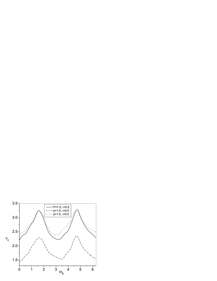
Figure 3: Plot of the critical value of coupling strengths $(\epsilon_{c})$ vs the frequency of identical oscillators $\omega_{0}$ for $D=1.0$ and $\tau_{d}=2.0$.

In this paper we consider the Kuramoto model of globally coupled (all-to-all) phase oscillators with a time delay and subject to the Ornstein-Uhlenbeck (OU) colored noise gardiner , that is a Gaussian process with a finite correlation time, and a non-Gaussian colored noise fuen ; 06preBag ; 07preBag ; bph . The focus in our study is on the interplay between the influence of noise and the time delay on the synchronization process. Our previous study on the stochastic Kuramoto model bph showed that the influence of the OU noise qualitatively differs from the case of white noise as the former allows for the full synchronization despite the fact that the system is subject to a noise, see e.g. Fig. 3 in bph .

Generally speaking, the time delay introduces de-phasing among the oscillators. This de-phasing is to interfere with the intrinsic correlations caused by the finite correlation time of the noise. As a result, we have found that the de-phasing plays important role in the dynamics of the system when the intrinsic correlations are small. We also investigate the effect of the time delay on the onset of synchronization for different noise strengths for both OU and non-Gaussian noises. But before doing that we show that the effect of time delay for the noiseless Kuramoto model is qualitatively equivalent to the effect of frequency fluctuations of the phase oscillators. Meanwhile we demonstrate that for the stochastic Kuramoto model the critical coupling grows nonlinearly with the increase of the time delay that is due to the additional de-phasing caused by the time delay. We also investigate how the transition from the Gaussian to a non-Gaussian noise changes the dynamical properties of the system.

II Stochastic Kuramoto model with time-delayed interactions

Let us consider the stochastic Kuramoto model with time-delayed interactions. This model describes $N$ coupled phase oscillators with dynamics governed by the following equations

$$\frac{d\theta_{i}(t)}{dt}=\omega_{i}+\frac{\epsilon}{N}\sum_{i<j}^{N}\sin[\theta_{j}(t-\tau_{d})-\theta_{i}(t)]+\eta_{i}(t),$$ (1)

where $\theta_{i}$ and $\omega_{i}$ are, respectively, the phase and the frequency of the $i$-th oscillators ($i=1,\dots,N$), $\epsilon$ is the coupling constant, and $\tau_{d}$ is the time delay. The independent noise processes $\eta_{i}(t)$ are governed by

$$\frac{d\eta_{i}(t)}{dt}=-\frac{1}{\tau}\frac{d}{d\eta_{i}}U_{p}(\eta_{i})+\frac{\sqrt{D}}{\tau}\xi_{i}(t).$$ (2)

The potential function is

$$U_{p}(\eta_{i})=\frac{D}{\tau(p-1)}\ln[1+\alpha(p-1)\eta_{i}^{2}/2]$$

with $\alpha=\tau/D$. $\xi_{i}(t)$ is the Gaussian white noise process defined via

$$\langle\xi_{i}(t)\xi_{j}(t^{\prime})\rangle=2\delta_{ij}\delta(t-t^{\prime})$$

and $\langle\xi_{i}(t)\rangle=0$. $D$ and $\tau$ measure the intensity and the correlation time of the noise process. Shortly we will discuss more about them. In the noise term in Eq. (1) it is apparent that in the present problem we assume the homogenous diffusion of phase oscillators.

The form of the noise $\eta_{i}$ allows us to control the deviation from the Gaussian behavior by changing a single parameter $p$. For $p=1$, Eq.(2) becomes

$$\frac{d\eta_{i}}{dt}=-\frac{\eta_{i}}{\tau}+\frac{\sqrt{D}}{\tau}\xi_{i}(t)$$ (3)

which is a well-known time evolution equation for the OU noise process gardiner for which the auto correlation function is given by

$$<\eta_{i}(t)\eta_{i}(t^{\prime})>=\frac{D}{\tau}\exp(-\frac{|t-t^{\prime}|}{\tau})\;\;.$$ (4)

Thus $D$ and $\tau$ are the noise strength and correlation time of the OU noise. The factor $[1+\alpha(p-1)\eta_{i}^{2}/2]$ in the first term of Eq.(2) leads to producing colored non Gaussian noise whose effective noise strength and correlation time are different from $D$ and $\tau$. However, to make the present paper self-consistent we would like to mention here salient features of the non-Gaussian noise only fuen .

The stationary probability distribution of the noise process is given by

$$P(\eta_{i})=\frac{1}{Z_{ip}}\left[1+\alpha(p-1)\frac{\eta_{i}^{2}}{2}\right]^{\frac{-1}{p-1}},$$ (5)

where $Z_{ip}$ is the normalization constant which equals to

$$Z_{ip}=\int_{-\infty}^{\infty}d\eta_{i}\left[1+\alpha(p-1)\frac{\eta_{i}^{2}}{2}\right]^{\frac{-1}{p-1}}$$

$$=\sqrt{\frac{\pi}{\alpha(p-1)}}\frac{\Gamma_{1}(1/(p-1)-1/2)}{\Gamma_{1}(1/(p-1))}\;\;\;,$$ (6)

with $\Gamma_{1}$ being the Gamma function. This distribution can be normalized only for $p<3$. Since $P(\eta_{i})$ is an even function of $\eta_{i}$, the first moment, $\langle\eta_{i}\rangle$, is always 0, and the second moment (variance) is given by

$$\langle\eta_{ip}^{2}\rangle=\frac{2D}{\tau(5-3p)}\;\;\;,$$ (7)

which is finite only for $p<5/3$. Furthermore, for $p<1$, the distribution has a cut-off and it is only defined for $|\eta_{i}|<\eta_{ic}\equiv\sqrt{\frac{2D}{\tau(1-p)}}$.

However, it is difficult to determine the auto correlation function (ACF) of the non Gaussian noise $\eta_{i}$ exactly. To have an idea about this we have calculated it numerically and presented the result in Fig. 1. The two time correlation function for the non Gaussian noise (solid curve) is fitted well by bi-exponentially decaying function $<\eta_{i}(t)\eta_{i}(0)>=ae^{-t/37}+be^{-t}$ having two correlation times 37 and 1, respectively, for $\tau=1.0$, where $a$ and $b$ are constants related to the noise intensity. In the same figure we have plotted numerically calculated ACF for Gaussian colored noise. It exactly mimics the function given in Eq.(4). Figure 1 clearly shows that the effective noise strength and correlation time for non Gaussian noise are greater compared to those of colored Gaussian one. The correlation time of non-Gaussian noise $\tau_{p}$ at the stationary regime of the process $\eta_{i}(t)$ diverges near $p=5/3$ and it can be approximated fuen over the range $1\leq p<5/3$ as

$$\tau_{p}\simeq 2\tau/(5-3p)\;\;.$$ (8)

This equation is qualitatively consistent with Fig.1. However, for this approximate correlation time, Eq.(7) becomes

$$\langle\eta_{ip}^{2}\rangle\simeq\frac{4D}{\tau_{p}(5-3p)^{2}}\;\;\;.$$ (9)

Equations (7-9) imply that when $p\rightarrow 1$, we recover the limit that $\eta_{i}$ is a Gaussian colored noise since at this limit Eqs.(7,9) correspond to the variance of Colored Gaussian noise as given in Eq.(4) and $\tau_{p}$ in Eq.(8) becomes $\tau$ which is the correlation time of the Gaussian noise. Another check in this context can be obtain in the following way. In this limit the term in the square bracket of Eq.(5) can be written as

$$1+\alpha(p-1){\eta_{i}^{2}}/{2}=\exp(\alpha(p-1){\eta_{i}^{2}}/{2})\;\;.$$ (10)

Then Eq.(5) becomes

$$P(\eta)=\frac{1}{Z_{1}}\exp(-\alpha\eta_{i}^{2}/2)\;\;\;,$$ (11)

with $Z_{1}=\sqrt{\pi/\alpha}$, which is a Gaussian distribution function. However, Eq.(7) shows that for a given external noise strength $D$ and the noise correlation time $\tau$, the variance of the non-Gaussian noise is higher than that of the Gaussian noise for $p>1$, i.e. $\langle\eta_{ip}^{2}\rangle>\langle\eta_{i1}^{2}\rangle$. Similarly, Eq.(8) implies that $\tau_{p}>\tau$ for $p>1$. These are consistent with the message of Fig. 1. Before leaving this issue we like to emphasize that in the present study we have considered continuous distribution of the non-Gaussian noise which is more relevant to the natural systems rather than two-state or discrete distributions as mostly used in the literature to study the noise driven dynamical systems doer .

The quantity of interest in the present study is

$$Z=\Gamma e^{i\Theta}=\frac{1}{N}\sum_{i=1}^{N}e^{i\theta_{i}}$$ (12)

which is the order parameter that measures the extent of synchronization in the system of $N$ phase oscillators. Its absolute value $\Gamma$ determines the degree of synchronization. It can be seen that in case of all the oscillators having the same phase the quantity equals to one ($\Gamma=1$) that corresponds to the full synchronization. The degree of synchronization is equal to zero ($\Gamma=0$) when all the oscillators are independent and have different phases. $\Theta$ defines an average phase of the oscillators. For the initial distribution of frequencies we choose the Lorentzian distribution

$$g(w)=\frac{1}{\pi}\frac{\lambda}{(\omega-\omega_{0})^{2}+\lambda^{2}}.$$ (13)

III Results and discussion

We have computed the order parameter $\Gamma$ as well as the critical coupling strength numerically since it is very difficult to study the problem analytically due to the colored noise and nonlinearity in terms of $\eta_{i}$ in its time evolution equation. Using Heun’s method (a stochastic version of the Euler method which reduces to the second order Runge-Kutta method in the absence of noise) we have solved the Eqs. (1) and (2) simultaneously rt . Based on the above method, we have studied time evolution of $N=5000$ coupled phase oscillators. In Ref. bph , we have showed that such a $N$ value is large enough so that the calculated quantities can represent those for systems in the thermodynamic limit.

For a given frequency distribution of the phase oscillators and environment of specific characteristic there exists a threshold value of the coupling strength $(\epsilon_{c})$ above which the coherent (synchronized) state is the stable state. If the $\epsilon$ is smaller than $\epsilon_{c}$, then the incoherent state is the stable one. $\epsilon_{c}$ is called critical coupling strength. To calculate the value of $\epsilon_{c}$, we first obtain the dependence of ensemble average of $\Gamma$ ($<\Gamma>$) on $\epsilon$. From this we determine numerically the derivative of $<\Gamma>$ with respect to $\epsilon$ at stationary state. The $\epsilon$ corresponding to the maximum value of the derivative is identified as the critical coupling strength. Our numerical study satisfies all the known limiting results, i.e., (i) $\epsilon_{c}=2\lambda$ in the absence of noise ($D=0$) and $\tau_{d}=0$ (ii) $\epsilon_{c}=2(\lambda+D)$ for white noise and $\tau_{d}=0$ (results are not shown here). We would also like to mention here that we chose stationary time to be a linear function of time delay ($\tau_{d}$) with the proportionality constant 100 and integration step length $h=0.01$.

We start our numerical study to determine how stability of both coherent and incoherent states depends on the time delay. Stability of these states of white-noise driven coupled oscillators in the Kuramoto model with a time delay has been studied by Young and Strogatz yeung . They have considered two cases. In the first case, all the oscillators are identical. In the second case, they have chosen Lorentzian distribution, Eq.(13), of frequency of the coupled oscillators. In the present paper, we extend this study to colored-noise driven coupled oscillators. The noise may be OU Gaussian or non Gaussian in characteristics. However, the critical coupling strength as mentioned above indicates that up to that value of coupling strength, the incoherent state can survive at long time. This range corresponds the stability zone of the incoherent state of the coupled phase oscillators. Thus critical coupling strength is a measure to imply how stability of incoherent or coherent states of the coupled oscillators depends on time delay and other parameters of the system. To demonstrate the dependence of the critical coupling strength $\epsilon_{c}$ on the time delay $\tau_{d}$ for various noise properties, we have reproduced Fig.2 of Ref. yeung for identical oscillators in the absence of noise (i.e. $D=0$) and presented it by the solid curve in Fig.2. In the presence of noise the phase oscillators become non identical and the time delay is effective in the dynamics even at its low value compared to the case where noise is absent. Since the variance of the non-Gaussian noise is higher compared to the Gaussian one, the shift of the damped oscillating curve towards the larger critical coupling strength from the noiseless case, is very big for former than latter at low noise correlation time, $\tau\approx 0.1$. Their difference reduces remarkably at large noise correlation time, $\tau\approx 2$. The reason may be the following. Effective noise correlation time of the colored non-Gaussian noise is much higher than the Gaussian one at large $\tau$. Increase of noise correlation time leads to develop better phase relationship among the oscillators reducing the phase diffusion. Thus at large $\tau$ the difference in critical coupling strength is small for a given time delay. It is apparent in Fig.2 that the interplay of noise correlation time and the time delay plays some constructive role to have a synchronized state particularly at large $\tau$ and around the first maximum of the damped oscillation curve. It also shifts a little bit the position of the maximum towards the left and reduces the oscillation amplitude at large time delay values. Thus colored noise plays a role beyond the induction of diffusion behavior.

Before going to the next case we would like to demonstrate the variation of critical coupling strength as a function of frequency of the coupled identical oscillators in the presence of time delay. In Fig.3 we have presented this. It exhibits that the variation is periodic as a result of interplay of the time delay and the frequency of the oscillator. However, again it shows how noise correlation can reduce the stability of incoherent state. Because of higher effective noise strength of the non-Gaussian noise, the critical coupling strength for the case $p=1.5$ and $\tau=0.5$ is comparable to white Gaussian noise.

For the second case of non-identical phase oscillators, we have done calculations similar to those for Fig. 2 for identical oscillators, and the results are presented in Fig. 4. Again, the solid curve in Fig.4 is a reproduction of Fig. 4 of Ref.yeung . All the features of Fig. 2 in the presence of colored noise has appeared in Fig. 4. Here one important point to be noted is that around the maximum, the incoherent state is unstable even at lower coupling strength in the presence of colored noise compared to the case without noise. Thus colored noise can effect the nonlinear coupling among the phase oscillators. It is quite similar to the modification of the dynamics by the colored noise in the presence of nonlinear potential han1 ; mb .

In the next step we demonstrate how the critical coupling strength varies as a function of noise parameters. First, we consider the dependence of $\epsilon_{c}$ on the noise strength (D). To identify the signature of the time delay in this context we have determined a ratio of critical coupling strengths $\epsilon_{c}(\tau_{d}=0)/\epsilon_{c}(\tau_{dm})$ for a given noise intensity, where $\tau_{dm}$ is the location of the first maximum in the $\tau_{d}$ axis. For identical oscillators we have chosen $\tau_{dm}=2$ from Fig. 2 and for nonidentical oscillators we have considered $\tau_{dm}=1$ from Fig. 4. It is not difficult to anticipate that this choice will incorporate the maximum effect of time delay. However, the ratio had been calculated for different values of the noise strength for the white noise and is presented in Fig.5. At first it rapidly increases both for identical (dotted curve) and nonidentical (solid curve) oscillators then the growth rate slows down. The initial growth rate is higher for identical oscillators compared to nonidentical oscillators because at low noise strength $\epsilon_{c}(\tau_{d}=0)$ is close to zero for the former and it grows at a faster rate. If the noise strength is appreciably large then the ratio is higher for identical oscillators than for the nonidentical case even if $\tau_{dm}$ is greater for the former than the latter. Thus time delay is more effective in the dynamics for nonidentical oscillators compared to the case of identical oscillators. Similar features are also observed for the colored noise and are demonstrated in insets (a) and (b) for the Gaussian and non-Gaussian noises. At large noise intensities the ratio of critical coupling strengths is smaller for the colored Gaussian noise compared to other noises for the case of nonidentical oscillators. Thus on switching from the white Gaussian to colored Gaussian or non-Gaussian characteristics of noise the time delay begins to play an important role in the dynamics.

The variation of the ratio of critical coupling strengths with the non-Gaussian parameter $p$ is demonstrated in Fig.6. It shows that the ratio increases as a function of $p$ for both cases of identical and nonidentical oscillators. The rate of growth is higher for the former than the latter case. The ratio is lower for the identical oscillators compared to the case of nonidentical oscillators at low $p$. However at large $p$ the situation turns around, it becomes inverse. These aspects can be understood if one keeps in mind that the effective noise strength increases as $p$ grows. Therefore Fig.5 is essentially similar to Fig.6 and it can be explained in the same way as we have explained the results presented in Fig.6.

Finally, in Fig.7 we have presented the variation of the ratio of critical coupling strength as a function of noise correlation time. It shows that the ratio decreases with increase of $\tau$. Since phase diffusion reduces as the noise becomes more colored, the critical coupling strength decreases as $\tau$ grows both in the presence and the absence of time delay. The ratio decreases because in the absence of time delay the colored noise is more effective in the dynamics. Similarly, the rate of decrease is a little bit higher for identical oscillators than for nonidentical ones. These kind of features are also observed for the colored non-Gaussian noise and are presented in the inset of the Fig. 7. In both cases the ratio is higher for the identical oscillators compared to the nonidentical oscillators for a given noise correlation time. Thus it again supports the statement that the time delay is more effective in the dynamics for the latter than for the former.

IV Conclusion

We have considered the stochastic Kuramoto model including time-delayed interaction with a delay time $\tau_{d}$ subject to both OU Gaussian or non-Gaussian colored noise with a correlated time $\tau$. The main focus of our study was on the interplay between the effects of finite correlation time $\tau$ and the time delay $\tau_{d}$ and their influence on the onset of the synchronization. Our results can be summarized as follows.

(i) The shift of the damped oscillating curve (for the critical coupling strength as a function of time delay $\tau_{d}$) towards the larger critical coupling strength from the noiseless case is very large for the non-Gaussian noise than for the Gaussian one at low noise correlation time, $\tau\approx 0.1$. Their difference reduces remarkably at large noise correlation times, $\tau\approx 2$ (Fig. 2).

(iii) Due to the present intrinsic correlations, the colored noise plays a role beyond the induction of diffusive behavior.

(iii) The incoherent (unsynchronized) state may be unstable around the maximum even at lower coupling strength values in the presence of colored noise compared to the noiseless case (Fig. 4).

(iv) The ratio of critical coupling strengths $\epsilon_{c}(\tau_{d}=0)/\epsilon_{c}(\tau_{dm})$ first rapidly increases as a function of noise intensity $D$ for both the identical and nonidentical oscillators and then slows down. The initial growth rate is higher for identical oscillators compared to the case of nonidentical oscillators. If the noise strength is appreciably large then the ratio is higher for identical oscillators than for the nonidentical case even if $\tau_{dm}$ is greater for the former than the latter case. At large values of noise intensity the ratio of critical coupling strength is smaller for the colored Gaussian noise than for the other noises for the case of nonidentical oscillators (Fig. 5).

(vi) The ratio of critical coupling strengths increases as a function of non-Gaussian parameter $p$ for both cases of identical and nonidentical oscillators. The rate of growth is higher for the former case than the latter one. The ratio is lower for identical oscillators compared to nonidentical oscillators at low $p\geq 1$. However at large values of $p$ it becomes inverse (Fig. 6).

(v) The above ratio decreases with increase of $\tau$. The rate of decrease is higher for the case of identical oscillators compared to the one for nonidentical oscillators (Fig. 7).

We anticipate that investigation of influence of time-delayed interactions and (generally non-Gaussian) noise in complex systems would lead to important insights into their stochastic dynamics, e.g., for the process of intercellular synchronization in biology zhou (see also systems biology models mentioned as possible applications in bph ). The time-delayed interaction also plays an important role in a molecular model of biological evolution 10pre06evo .

This work was supported by the National Science Council in Taiwan under Grant Nos. NSC 96-2911-M 001-003-MY3 & NSC 98-2811-M-001-066, and National Center for Theoretical Sciences in Taiwan.

Figure 1: Two-time correlation function vs. $t$ of both Gaussian ($p=1$) and non-Gaussian ($p=1.5$) colored noises for parameters $\tau=1.0$ and $D=0.5$.

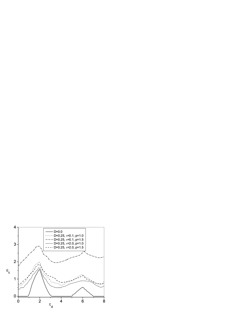
Figure 2: Plot of the critical value of coupling strength $\epsilon_{c}$ vs the time delay $\tau_{d}$ for the identical oscillators for $\omega_{0}=\pi/2$.

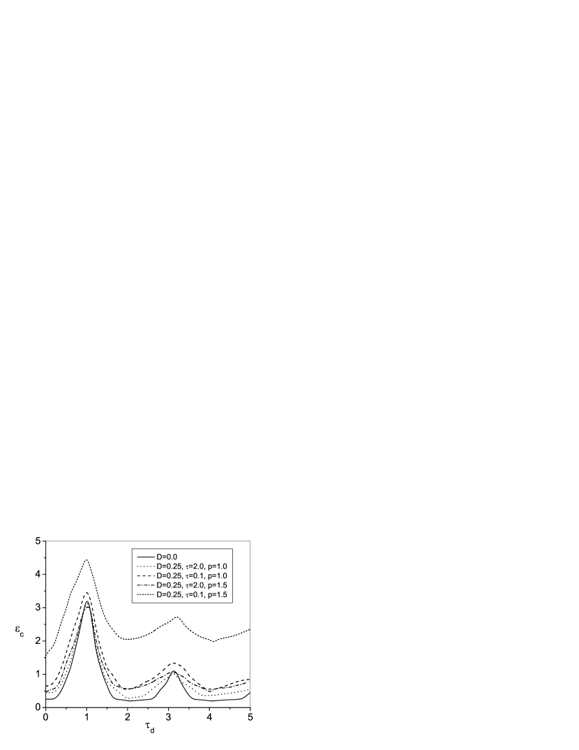
Figure 4: Plot of the critical value of coupling strength $\epsilon_{c}$ vs the time delay $\tau_{d}$ for the nonidentical oscillators for the parameter set $\omega_{0}=3.0$ and $\lambda=0.1$.

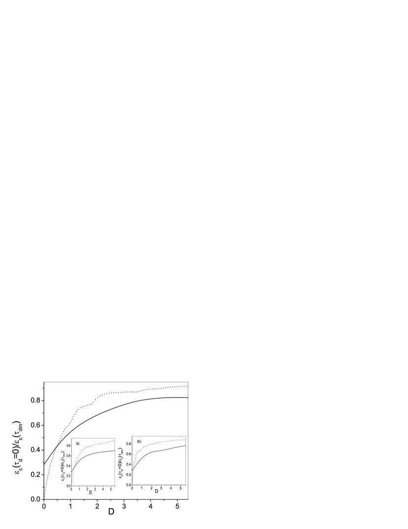
Figure 5: Plot of the ratio of the critical value of coupling strengths $\epsilon_{c}(\tau_{d}=0)/\epsilon_{c}(\tau_{dm})$ vs the noise intensity $D$ for the parameter set $p=1.0$ and $\tau=0.0$. For identical oscillators $\omega_{0}=\pi/2$ and that of nonidentical oscillators, $\omega_{0}=3.0$, $\lambda=0.5$. Solid and dotted curves correspond to nonidentical and identical oscillators, respectively. The insets contain results for different parameter sets: (a) $p=1.0$ and $\tau=0.5$, (b) $p=1.5$ and $\tau=0.5$

Figure 6: Plot of the ratio of the critical value of coupling strengths $\epsilon_{c}(\tau_{d}=0)/\epsilon_{c}(\tau_{dm})$ vs the non-Gaussian parameter $p$ for the parameter set $\tau=0.5$ and $D=0.25$. For identical oscillators $\omega_{0}=\pi/2$ and that of nonidentical oscillators $\omega_{0}=3.0$ and $\lambda=0.5$. Solid and dotted curves correspond to nonidentical and identical oscillators, respectively.

Figure 7: Plot of the ratio of the critical value of coupling strengths $(\epsilon_{c}(\tau_{d}=0)/\epsilon_{c}(\tau_{dm}))$ vs the noise correlation time $\tau$ for the parameter set $p=1.0$ and $D=1.0$. For identical oscillators $\omega_{0}=\pi/2$ and that of nonidentical oscillators $\omega_{0}=3.0$ and $\lambda=0.5$. Solid and dotted curves correspond to nonidentical and identical oscillators, respectively. In the inset, $p=1.5$.

References

- (1) Winfree A T 1967 J. Theor. Biol. 16 15 Winfree A T 1980 The Geometry of Biological Time (Springer, New York)
- (2) Kuramoto Y 1984 Prog. Theor. Phys. Suppl. 79 223 Kuramoto Y 1984Chemical Oscillations, Waves, and Turbulence (Springer-Verlag, New York) Kuramoto Y and Nishikawa I 1987 J. Stat. Phys. 49 569
- (3) Strogatz S H 2000 Physica (Amsterdam) 143D 1
- (4) Pikovsky A, Rosenblum M, and Kurths J 2001 Synchronization - A Universal Concept in Nonlinear Sciences (Cambridge University Press, Cambridge)
- (5) Manrubia S C, Mikhailov A S and Zanette D H 2004 Emergence of Dynamical Order: Synchronization Phenomena in Complex Systems (World Scientific, Singapore)
- (6) Acebron J J, Bonilla L L, Perez-Vicente C J, Ritort F and Spigler R 2005 Rev. Mod. Phys. 77 137
- (7) Kaneko K 1990 Phys. Rev. Lett. 65 1391
- (8) Pecora L M and Caroll T L 1998 Phys. Rev. Lett. 80 2109
- (9) Gade P M and Hu C-K 1999 Phys. Rev. E. 60 4966 Gade P M and Hu C-K 2000 Phys. Rev. E. 62 6409 Gade P M and Hu C-K 2006 Phys. Rev. E. 73 036212 Jalan S, Amritkar R E and Hu C-K 2005 Phys. Rev. E. 72 016211 Amritkar R E, Jalan S and C.-K. Hu C-K 2005 Phys. Rev. E 72 016212 Hung Y-C, Huang Y-T, Ho M-C, and Hu C-K 2008 Phys. Rev. E 77 016202
- (10) Hong H, Choi M Y and Kim B J 2002 Phys. Rev. E 65 026139 Hong H, Chate H, Park H and Tang LH 2007 Phys. Rev. Lett. 99 184101 Hong H, Park H and Tang LH 2007 Phys. Rev. E 76 066104
- (11) Wu M-C and Hu C-K 2006 Phys. Rev. E 73 051917
- (12) Niebur E, Schuster H G, and Kammen D M 1991 Phys. Rev. Lett. 67 2753
- (13) Nakamura Y, Tominaga F and Munakata T 1994 Phys. Rev. E 49 4849
- (14) Yeung M K S and Strogatz S H 1999 Phys. Rev. Lett. 82 648
- (15) Choi M Y, Kim H J, Kim D and Hong H 2000 Phys. Rev. E 61 371
- (16) Haken H 2002 Brain Dynamics: Synchronization and Activity Patterns in Pulse-Coupled Neural Nets with Delays and Noise (Springer-Verlag, Berlin)
- (17) Gardiner C W 2004 Handbook of Stochastic Methods, 3rd ed. (Springer-Verlag, Berlin)
- (18) See Fuentes M A, Wio H S and Toral R 2002 Physica A 303 91 for details on the non-Gaussian noise
- (19) Bag B C and Hu C-K 2006 Phys. Rev. E 73 061107
- (20) Bag B C and Hu C-K 2007 Phys. Rev. E 75 042101
- (21) Bag B C, Petrosyan K G and Hu C-K 2007 Phys. Rev. E 76 056210
- (22) Hänggi P, Talkner P and Borkovec M 1990 Rev. Mod. Phys. 62 251 Doering C R and J. C. Gadoua J C 1992 Phys. Rev. Lett 69, 2318 Reimann P 2002 Phys. Rep. 361 265
- (23) Toral R 1995 in Computational Physics, Lecture Notes in Physics, Vol.448 (Springer-Verlag, Berlin) Eds. Garrido P and Marro J
- (24) Hänggi P 1994 Chem. Phys. 180 157
- (25) Sen M K and Bag B C 2009 Euro. Phys. J. B 68 253
- (26) Zhou T, Chen L and Aihara K 2005 Phys. Rev. Lett. 95 178103
- (27) Saakian D B, Martirosyan A S and Hu C-K 2010 Phys. Rev. E 81 061913