Moments of GPDs and transverse-momentum dependent PDFs from the lattice

Abstract:

I review lattice-QCD calculations of the electromagnetic and generalized form factors (GFFs), which determine the transverse structure of the nucleon, and briefly comment on recent calculations related to transverse-momentum dependent parton distribution functions (TMDPDFs).

Lattice QCD calculations of hadron structure have been carried out for two decades, see [1] for a recent review. As the up- and down-quark masses are gradually lowered toward the physical point (isospin symmetry is assumed), new questions have arisen on the way. The calculations have reached a certain degree of maturity and consensus among different collaborations down to about $m_{\pi}=300$MeV. With the goal in mind of confronting the lattice results with hadron phenomenology, it is useful to first discuss the quantities that are well determined experimentally. Such quantities include the axial charge of the nucleon, the isovector momentum fraction and the electromagnetic (e.m.) form factors (FFs). One may then focus on quantities where the lattice can be a discovery tool, such as the generalized form factors.

I therefore start by discussing the calculation of e.m. FFs, both because they are a special case of the GFFs and because they represent a benchmark calculation of experimentally well-determined functions. The matrix elements of the e.m. current between two nucleon states are parametrized by the Dirac and Pauli form factors ($q=P^{\prime}-P$, $Q^{2}=-q^{2}$),

$$\langle P^{\prime},\Lambda^{\prime}|J^{\mu}|P,\Lambda\rangle=\bar{U}(P^{\prime},\Lambda^{\prime})\Gamma^{\mu}(q^{2})U(P,\Lambda)\,,~{}~{}~{}~{}~{}~{}~{}\Gamma^{\mu}(q^{2})=\gamma^{\mu}{F_{1}}(Q^{2})+i\sigma^{\mu\nu}\frac{q_{\nu}}{2m}{F_{2}}(Q^{2}).$$ (1)

The result of a calculation at $m_{\pi}=300$MeV by the LHP collaboration is displayed in Fig. (1, top row). It uses 2+1 flavors of domain-wall fermions at a lattice spacing of $a=0.084$fm. Several other collaborations have obtained the FFs at similar pion masses [2]. A common point among these calculations is that the dipole form fits the data well, but the radii extracted from the fits are significantly smaller than the phenomenological radii. Secondly, chiral effective theory predicts a strong pion mass dependence of the Dirac and Pauli radii, but the lattice data exhibits a much milder dependence. It may be that the $m_{\pi}$-range of applicability of the chiral formulae is much smaller than 300MeV. Finite-volume effects need to be investigated in more detail too.

The approximate dipole behavior of the phenomenological FF $F_{1}(Q^{2})=\frac{1}{1+Q^{2}/0.71{\rm GeV}^{2}}$ can be understood as being due to the contribution of two nearby vector meson poles with opposite residua [3]. Figure (1, bottom row) illustrates the fact that in Nature, the Dirac dipole mass lies within $10\%$ of the $\rho$ meson mass. In QCD at larger $m_{u,d}$ however, lattice results show that the Dirac dipole mass is significantly larger than the vector meson mass in the same theory. We note that, since both the Dirac and Pauli radii diverge in the chiral limit, the latter must become very large compared to the $\rho$ Compton wavelength approaching the chiral limit.

The numerical evaluation of Wick-connected and -disconnected diagrams that contribute to three-point functions (Fig. (1), bottom row) proceeds in a rather different way. Most collaborations have focused on the more tractable connected contributions, thus restricting themselves to isovector quantities. Consider in this respect the flavor structure of the e.m. FFs of the proton,

$$F_{1,2} = {\textstyle\frac{2}{3}}F^{u}-{\textstyle\frac{1}{3}}F^{d}-{\textstyle\frac{1}{3}}F^{s}={\textstyle\frac{1}{2}}F^{u-d}+{\textstyle\frac{1}{6}}F^{u+d-2s}={\textstyle\frac{1}{2}}F^{u-d}_{\rm conn}+{\textstyle\frac{1}{6}}F^{u+d}_{\rm conn}+{\textstyle\frac{1}{6}}(F^{u+d}_{\rm disc}-2F^{s}_{\rm disc}).$$

Figure (1, middle row), displaying the strangeness FFs [4], suggests that disconnected diagrams contribute less than $0.01$ to $F_{1}$, which is negligible at low $Q^{2}$ compared to the other uncertainties.

   

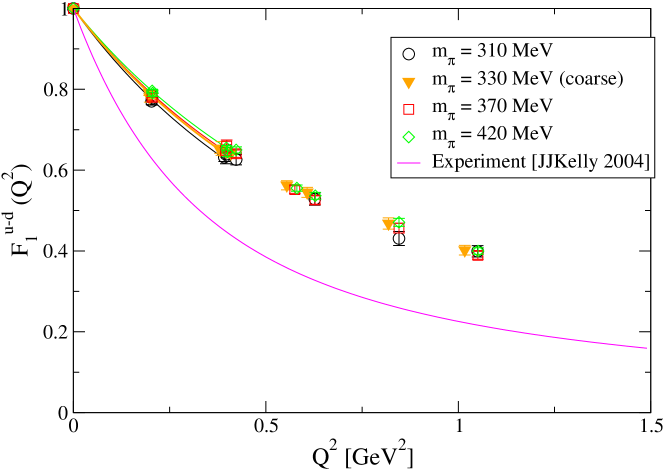
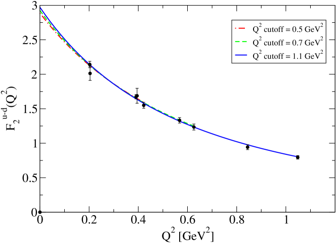
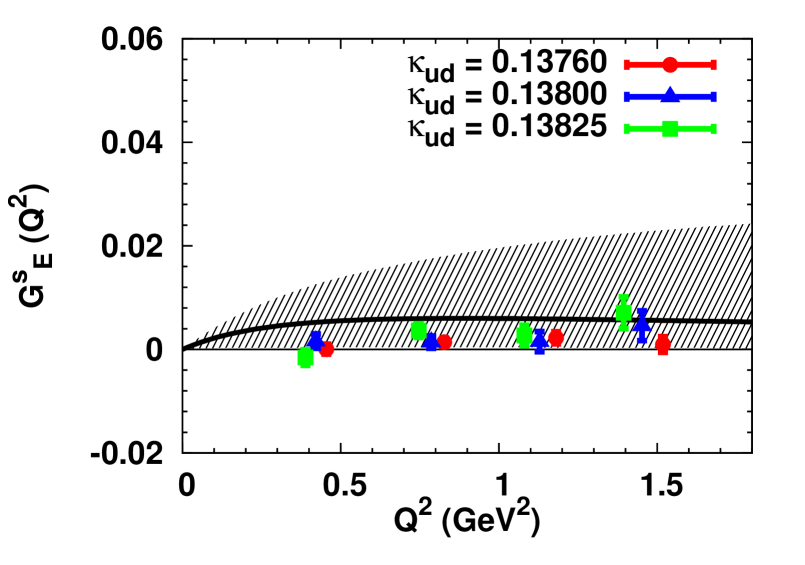
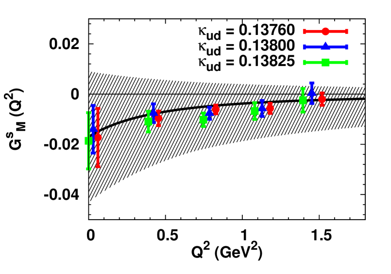
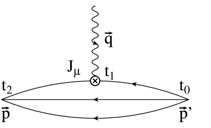
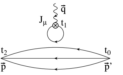
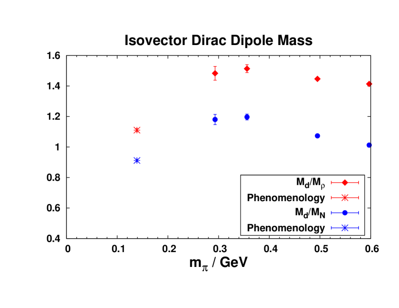
Figure 1: Top row: the e.m. FFs in an $\mathop{N_{\rm f}}=2+1$ calculation using domain-wall fermions at a lattice spacing 0.084fm (0.114fm in the ‘coarse’ case). The right plot displays the Pauli FF calculated at $m_{\pi}=300$MeV [5]. Middle row: calculation of the strangeness FF of the nucleon by the $\chi$QCD collaboration [4] ($N_{\rm f}=2+1$, $a=0.12$fm, $m_{\pi}\geq 600$MeV). Bottom row: connected and disconnected Wick contractions contributing to hadronic matrix elements (fig. from [4]). Right, the nucleon Dirac dipole mass [6].

I now briefly describe the connection between the generalized parton distributions (GPDs), which govern Deeply Virtual Compton Scattering, and the GFFs that can be computed on the lattice. The GPDs parametrize the matrix elements of the operators

$${\cal O}_{\Gamma}(x)=\int\!\frac{d\lambda}{4\pi}e^{i\lambda x}\overline{q}(\frac{-\lambda n}{2})\Gamma\,{\cal P}e^{-ig\int_{-\lambda/2}^{\lambda/2}d\alpha\,n\cdot A(\alpha n)}\!q(\frac{\lambda n}{2})\,.$$ (2)

Here $n$ is a light cone vector, $/\!\!\!{n}\equiv n_{\mu}\gamma_{\mu}$, and in the following $x$ is the momentum fraction, $\Delta\equiv P^{\prime}-P$, $t=\Delta^{2}$ and $\xi=-n\cdot\Delta/2$. Different $\Gamma$ matrices lead to different GPDs,

$$\Gamma=/\!\!\!{n}\leadsto(H,E),~{}~{}~{}~{}~{}\Gamma=/\!\!\!{n}\gamma_{5}\leadsto(\widetilde{H},\widetilde{E}),~{}~{}~{}~{}~{}\Gamma=n_{\mu}\sigma^{\mu j}\leadsto(H_{T},E_{T})~{}{\rm and}~{}(\widetilde{H}_{T},\widetilde{E}_{T}).$$ (3)

For $\Gamma\doteq/\!\!\!{n}$, the ‘unpolarized’ case, the parametrization at a renormalization scale $\mu$ takes the form

$$\left\langle P^{\prime},\Lambda^{\prime}\right|{\cal O}_{\not n}(x,\mu)\left|P,\Lambda\right\rangle=\langle\!\langle/\!\!\!{n}\rangle\!\rangle H(x,\xi,t,\mu)+\frac{n_{\mu}\Delta_{\nu}}{2m}\langle\!\langle i\sigma^{\mu\nu}\rangle\!\rangle E(x,\xi,t,\mu)\,,$$ (4)

where $\langle\!\langle\Gamma\rangle\!\rangle\equiv\overline{U}(P^{\prime},\Lambda^{\prime})\Gamma U(P,\Lambda)$ and $U(P,\Lambda)$ is a spinor that solves the free Dirac equation. GPDs determine the distribution of partons and their helicities in impact parameter space [7],

$$q(x,{\bf b}_{\perp})={\textstyle\int\frac{\,\mathrm{d}^{2}{\bf b}_{\perp}}{(2\pi)^{2}}}\,e^{-i\Delta_{\perp}\cdot{\bf b}_{\perp}}\,H(x,\xi=0,-\Delta_{\perp}^{2})\,,~{}~{}~{}\Delta q(x,{\bf b}_{\perp})={\textstyle\int\frac{\,\mathrm{d}^{2}{\bf b}_{\perp}}{(2\pi)^{2}}}\,e^{-i\Delta_{\perp}\cdot{\bf b}_{\perp}}\,\widetilde{H}(x,\xi=0,-\Delta_{\perp}^{2})\,.$$

Mellin-moments of the GPDs, $H^{n}(\xi,t)\equiv{\textstyle\int_{-1}^{1}}\,\mathrm{d}x\,x^{n-1}H(x,\xi,t)$, are given by polynomials in the longitudinal momentum transfer $\xi$,

$$\begin{array}[]{l@{~~}l@{~~}l@{~~}l}H^{n=1}(\xi,t)\hfil~{}~{}&={A_{10}(t)},\hfil~{}~{}&E^{n=1}(\xi,t)\hfil~{}~{}&={B_{10}(t)},\\ H^{n=2}(\xi,t)\hfil~{}~{}&={A_{20}(t)}+(2\xi)^{2}{C_{20}(t)},\hfil~{}~{}&E^{n=2}(\xi,t)\hfil~{}~{}&={B_{20}(t)}-(2\xi)^{2}{C_{20}(t)},\\ H^{n=3}(\xi,t)\hfil~{}~{}&={A_{30}(t)}+(2\xi)^{2}{A_{32}(t)}\,,\hfil~{}~{}&E^{n=3}(\xi,t)\hfil~{}~{}&={B_{30}(t)}+(2\xi)^{2}{B_{32}(t)}\,,~{}\dots\end{array}$$ (5)

The coefficients of these polynomials are the GFFs calculated on the lattice. In the $n=1$ case, $A_{10}$ and $B_{10}$ coincide with $F_{1}$ and $F_{2}$. In the $n=2$ unpolarized case, the operator is ${\cal O}_{\mu_{1}\mu_{2}}(x)=\frac{1}{2}\bar{q}(\gamma_{\mu_{1}}{D}_{\mu_{2}}+\gamma_{\mu_{2}}{D}_{\mu_{1}})q\,$ and, with $\bar{P}\equiv(P+P^{\prime})/2$,

$$\langle P^{\prime}|{\cal O}_{\mu_{1}\mu_{2}}(q)|P\rangle=\bar{P}_{\{\mu_{1}}\langle\!\langle\gamma_{\mu_{2}\}}\rangle\!\rangle\,{A_{20}(t)}+{\textstyle\frac{i}{2m}}\bar{P}_{\{\mu_{1}}\langle\!\langle\sigma_{\mu_{2}\}\alpha}\rangle\!\rangle\Delta_{\alpha}\,{B_{20}(t)}+{\textstyle\frac{1}{m}}\Delta_{\{\mu_{1}}\Delta_{\mu_{2}\}}\,{C_{20}(t)}\,.$$ (6)

The forward-limit of $A_{20}$ and $B_{20}$ determine the momentum and spin decomposition of the nucleon in terms of quark and gluon contributions [8]. In practice, only the first few moments $n\leq 3$ are accessible on the lattice. The impact-parameter dependence ${\bf b}_{\perp}$ can be obtained more easily, currently $(0.4{\rm GeV})^{2}<\Delta_{\perp}^{2}<(2.0{\rm GeV})^{2}$. The lower end of this interval is limited by momentum quantization in a finite box, $P=\frac{2\pi k}{L}$, $k\in\mathbb{Z}$. It can potentially be overcome with twisted boundary conditions, whereby $P=\frac{\theta}{L}+\frac{2\pi k}{L}$ [9]. The upper end is limited by the inverse lattice spacing.

Figure (2, left panel) displays the $n=1,2$ and 3 GFFs of the nucleon (isovector, unpolarized case). This particular calculation is performed in a (3.5fm)³ box at a pion mass of 355MeV. For the purpose of the comparison, the FFs have been normalized by their forward value. It is clearly seen that the FFs become flatter as $n$ increases. This translates into decreasing transverse radii, (right panel). The latter have been obtained by performing dipole fits to the FF data with $|t|\leq 0.5{\rm GeV}^{2}$. The simulations are performed in boxes of size (2.5fm)³, with in addition a (3.5fm)³ simulation at $m_{\pi}=355$MeV. In the $n=1$ case, a gradual increase in the (Dirac) radius is observed as the pion mass is lowered toward its physical value. For $n\geq 2$, this growth in the transverse size of the nucleon is not observed in the range of explored pion masses. This is qualitatively consistent with the expectation from chiral effective theory, which predicts a logarithmic divergence in the $n=1$ case, but finite values for the radii corresponding to higher $n$. However, at $m_{\pi}=355$MeV one also observes a statistically significant difference between the radii extracted from volumes (2.5fm)³ and (3.5fm)³. Since the finite-size effect is expected to increase when the pion mass decreases, it appears necessary to check the observed trends by using large-volume simulations.

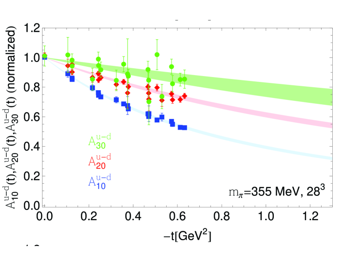
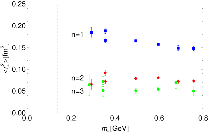
Figure 2: Left: Unpolarized isovector GFFs. Right: the corresponding radii [6].

In conclusion, GPDs play a central role in describing quantitatively the three-dimensional structure of the nucleon. Lattice QCD is ideally suited to determine the GFFs associated with their low Mellin-moments. A handful of lattice collaborations have published results for the nucleon structure for pion masses down to about 300MeV. A general observation is that many observables show a very mild pion mass dependence. The non-analytic pion-mass dependence predicted by chiral effective theory is not yet visible in the data; presumably it sets in at a lower pion mass. The next step will therefore be to go down to 200MeV [10] with controlled uncertainties, in particular a solid understanding of the finite-volume effects in the simulations is crucial.

The formalism to study transverse-momentum dependent PDFs on the lattice, relevant to semi-inclusive DIS, has recently been studied [11]. One important aspect of the calculation is the renormalization of non-local operators of the type $\bar{q}(x)\Gamma\,U_{x,0}q(0)$, where $U_{x,0}$ is a Wilson line. A second essential issue is the connection between the matrix elements of this operator with $U_{x,0}$ along the light-cone and with $U$ in the Euclidean domain. I expect to see further developments in this field in the near future.

References

- [1] P. Hagler, Hadron structure from lattice quantum chromodynamics, Phys. Rept. 490 (2010) 49–175, [arXiv:0912.5483].
- [2] T. Yamazaki et. al., Nucleon form factors with 2+1 flavor dynamical domain-wall fermions, Phys. Rev. D79 (2009) 114505, [arXiv:0904.2039].
- [3] C. F. Perdrisat, V. Punjabi, and M. Vanderhaeghen, Nucleon electromagnetic form factors, Prog. Part. Nucl. Phys. 59 (2007) 694–764, [hep-ph/0612014].
- [4] T. Doi et. al., Nucleon strangeness form factors from Nf=2+1 clover fermion lattice QCD, Phys. Rev. D80 (2009) 094503, [arXiv:0903.3232].
- [5] S. N. Syritsyn et. al., Nucleon Electromagnetic Form Factors from Lattice QCD using 2+1 Flavor Domain Wall Fermions on Fine Lattices and Chiral Perturbation Theory, Phys. Rev. D81 (2010) 034507, [arXiv:0907.4194].
- [6] LHPC Collaboration, J. D. Bratt et. al., Nucleon structure from mixed action calculations using 2+1 flavors of asqtad sea and domain wall valence fermions, arXiv:1001.3620.
- [7] M. Burkardt, Impact parameter dependent parton distributions and off- forward parton distributions for zeta –¿ 0, Phys. Rev. D62 (2000) 071503, [hep-ph/0005108].
- [8] X.-D. Ji, Gauge invariant decomposition of nucleon spin, Phys. Rev. Lett. 78 (1997) 610–613, [hep-ph/9603249].
- [9] QCDSF and UKQCD Collaboration, M. Gockeler et. al., Nucleon structure with partially twisted boundary conditions, PoS LATTICE2008 (2008) 138.
- [10] QCDSF/UKQCD Collaboration, M. Gockeler et. al., Lattice Investigations of Nucleon Structure at Light Quark Masses, arXiv:0912.0167.
- [11] P. Hagler, B. U. Musch, J. W. Negele, and A. Schafer, Intrinsic quark transverse momentum in the nucleon from lattice QCD, Europhys. Lett. 88 (2009) 61001, [arXiv:0908.1283].