Spontaneous breaking of superconformal invariance in (2+1)D supersymmetric Chern-Simons-matter theories in the large N limit

Abstract

In this work we study the spontaneous breaking of superconformal and gauge invariances in the Abelian ${\cal N}=1,2$ three-dimensional supersymmetric Chern-Simons-matter (SCSM) theories in a large $N$ flavor limit. We compute the Kählerian effective superpotential at subleading order in $1/N$ and show that the Coleman-Weinberg mechanism is responsible for the dynamical generation of a mass scale in the ${\cal{N}}=1$ model. This effect appears due to two-loop diagrams that are logarithmic divergent. We also show that the Coleman-Weinberg mechanism fails when we lift from the ${\cal{N}}=1$ to the ${\cal{N}}=2$ SCSM model.

I Introduction

The $AdS/CFT$ correspondence which relates a special weak (strong) coupled string theory to a strong (weak) coupled superconformal field theory Maldacena:1997re , opened a new freeway in the direction of the understanding of strong coupled gauge field theories. Several aspects of the correspondence have been studied  Gubser:1998bc ; Witten:1998qj . In particular, the $AdS_{4}/CFT_{3}$ correspondence have attracted great attention in the literature due to its contribution for the development of the understanding of some condensed matter effects, especially the superfluidity sf and the superconductivity sc ; Aprile:2010yb . Recently, Gaiotto and Yin suggested that various ${\cal{N}}=2,3$ three-dimensional SCSM theories are dual to open or closed string theories in $AdS4$ Gaiotto:2007qi . These SCSM model are superconformal invariants, an essential ingredient to relate them to $M2$ branes Bagger:2006sk ; Krishnan:2008zm ; Gustavsson:2007vu .

On the other hand, it is known that in a three-dimensional non-supersymmetric Chern-Simons-matter theory the conformal symmetry is dynamically broken Dias:2003pw by the Coleman-Weinberg mechanism  Coleman:1973jx in two loop approximation; the same is also true for the superconformal invariance of the Abelian, $D=(2+1)$, ${\cal{N}}=1$ SCSM model  Ferrari:2010ex , after two loops corrections to the effective (super) potential. For the ${\cal{N}}=2$ model, on the other hand, this mechanism fails to induce a breakdown of this symmetry.

In this work we study the spontaneous breaking of the superconformal and gauge invariances in the three-dimensional Abelian ${\cal{N}}=1,2$ SCSM theories in the large $N$ flavor limit approximation. In the section II it is shown that the dynamical breaking of superconformal and gauge invariances in the ${\cal{N}}=1$ SCSM model is compatible with $1/N$ expansion, determining that the matter self-interaction coupling constant $\lambda$ must be of the order of $g^{6}/N$, while no restriction to the gauge coupling $g$ has to be imposed. In the section III, it is discussed that similarly to what happens in the perturbative approach  Ferrari:2010ex the Coleman-Weinberg mechanism in the $1/N$ expansion is not feasible for the ${\cal{N}}=2$ extension of SCSM model. This happens because the coupling constants are constrained by the conditions that minimize the effective superpotential. In the section IV the last comments and remarks are presented.

II ${\cal{N}}=1$ SUSY Chern-Simons-matter model

The ${\cal{N}}=1$ three-dimensional supersymmetric Chern-Simons-matter model (SCSM) is defined by the classical action

$$S=\int{d^{5}z}\Big{\{}-\frac{1}{2}\Gamma^{\alpha}W_{\alpha}-\frac{1}{2}\overline{\nabla^{\alpha}\Phi_{a}}\nabla_{\alpha}\Phi_{a}+\lambda(\bar{\Phi}_{a}\Phi_{a})^{2}\Big{\}}\leavevmode\nobreak\ ,$$ (1)

where $W^{\alpha}=(1/2)D^{\beta}D^{\alpha}\Gamma_{\beta}$ is the gauge superfield strength with $\Gamma_{\beta}$ being the gauge superfield, $\nabla^{\alpha}=(D^{\alpha}-ig\Gamma^{\alpha})$ is the supercovariant derivative, and $a$ is an index that assume values from $1$ to $N$, where $N$ is the number of flavors of the complex superfields $\Phi$. We use the notations and conventions as in Gates:1983nr . When a mass term $\mu(\bar{\Phi}_{a}\Phi_{a})$, with $\mu>0$, is present in the matter sector, the SCSM model exhibits spontaneous breaking of gauge invariance and a consequent generation of mass for the scalar and gauge superfields at tree level Lehum:2007nf .

We are dealing with a classically superconformal model, and our aim in this work is to look for the possibility of dynamical breaking of the superconformal and gauge invariances in the $1/N$ expansion. To do this, let us redefine our coupling constants, $\lambda\rightarrow\dfrac{\lambda}{N}$, $g\rightarrow\dfrac{g}{\sqrt{N}}$, and shift the $N$-th component of the set of superfields $\Phi_{a}$ ($\bar{\Phi}_{a}$) by the classical background superfield $\sigma_{cl}=\sigma_{1}-\theta^{2}\sigma_{2}$ as follows

$$\bar{\Phi}_{N} = \frac{1}{\sqrt{2}}\Big{(}\Sigma+\sqrt{N}\sigma_{cl}-i\Pi\Big{)}\leavevmode\nobreak\ ,$$

$$\Phi_{N} = \frac{1}{\sqrt{2}}\Big{(}\Sigma+\sqrt{N}\sigma_{cl}+i\Pi\Big{)}\leavevmode\nobreak\ ,$$ (2)

with the vacuum expectation values (VEV) of the quantum superfields, i.e., $\langle\Sigma\rangle=\langle\Pi\rangle=\langle\Phi_{j}\rangle=0$ vanishing at any order of $1/N$. The index $j$ runs over: $j=1,2,\cdots(N-1)$. To investigate the possibility of spontaneous breaking of gauge/superconformal symmetry is enough to obtain the Kählerian superpotential Burgess:1983nu ; Ferrari:2010ex , i.e., to consider the the contributions to the superpotential, where supersymmetric derivatives ($D^{\alpha}$,$D^{2}$) acts only on the background superfield $\sigma_{cl}$.

The action written in terms of the real quantum superfields $\Sigma$ and $\Pi$ and the $(N-1)$ complex superfields $\Phi_{j}$ with vanishing VEVs is given by

$$S = \int{d^{5}z}\Big{\{}-\dfrac{1}{2}\Gamma^{\alpha}W_{\alpha}-\frac{g^{2}\sigma_{cl}^{2}}{2}\Gamma^{2}+\frac{g}{2}\left(\sigma_{cl}D^{\alpha}\Pi\Gamma_{\alpha}+\Pi\Gamma_{\alpha}D^{\alpha}\sigma_{cl}\right)+\bar{\Phi}_{j}(D^{2}+\lambda\sigma_{cl}^{2})\Phi_{j}+\frac{1}{2}\Sigma(D^{2}+3\lambda\sigma_{cl}^{2})\Sigma$$ (3)

$$+\frac{1}{2}\Pi(D^{2}+\lambda\sigma_{cl}^{2})\Pi+i\frac{g}{2\sqrt{N}}\Big{(}D^{\alpha}\bar{\Phi}_{j}\Gamma_{\alpha}\Phi_{j}+\bar{\Phi}_{j}\Gamma_{\alpha}D^{\alpha}\Phi_{j}\Big{)}+\frac{g}{2\sqrt{N}}\left(D^{\alpha}\Pi\Gamma_{\alpha}\Sigma+\Pi\Gamma_{\alpha}D^{\alpha}\Sigma\right)$$

$$-\dfrac{g^{2}}{2N}\left(2\bar{\Phi}_{j}\Phi_{j}+\Sigma^{2}+\Pi^{2}\right)\Gamma^{2}+\dfrac{\lambda}{N}\left(\bar{\Phi}_{j}\Phi_{j}\right)^{2}+\dfrac{\lambda}{4N}\left(\Sigma^{2}+\Pi^{2}\right)^{2}+\dfrac{\lambda}{N}\left(\Sigma^{2}+\Pi^{2}\right)\bar{\Phi}_{j}\Phi_{j}$$

$$+\dfrac{\lambda}{\sqrt{N}}\sigma_{cl}\Sigma\left(2\bar{\Phi}_{j}+\Sigma^{2}+\Pi^{2}-\dfrac{g^{2}}{\lambda}\Gamma^{2}\right)+\sqrt{N}\left(\lambda\sigma_{cl}^{3}+D^{2}\sigma_{cl}\right)\Sigma+N\sigma_{cl}D^{2}\sigma_{cl}+N\dfrac{\lambda}{4}\sigma_{cl}^{4}$$

$$-\frac{1}{4\alpha}(D^{\alpha}\Gamma_{\alpha}+\alpha{g\sigma_{cl}}\Pi)^{2}+\bar{c}D^{2}c+\alpha\frac{g^{2}\sigma_{cl}^{2}}{2}\bar{c}c+\frac{\alpha}{2\sqrt{N}}{g^{2}\sigma_{cl}}\bar{c}\Sigma c+\mathcal{L}_{ct}\Big{\}}\leavevmode\nobreak\ ,$$

where the last line of above equation is the $R_{\xi}$ gauge-fixing term and the corresponding Faddeev-Popov terms, plus counterterms of renormalization represented by $\mathcal{L}_{ct}$. The term $\dfrac{-g\sigma_{cl}}{2}D^{\alpha}\Pi\Gamma_{\alpha}$ is responsible for the mixing between the scalar superfield $\Pi$ and the gauge superfield $\Gamma^{\alpha}$. The introduction of an $R_{\xi}$ gauge-fixing eliminate this mixing, in the approximation considered.

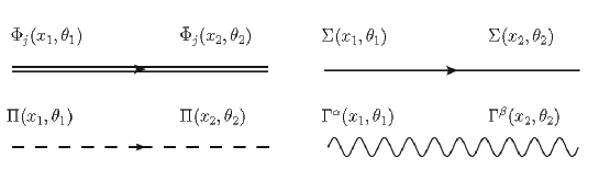
Figure 1: Propagators.

From the action above, Eq.(3), we can compute the free propagators, Figure1, of the model as

$$\langle T\leavevmode\nobreak\ \Phi_{i}(k,\theta)\bar{\Phi}_{j}(-k,\theta^{\prime})\rangle = -i\delta_{ij}\frac{D^{2}-M_{0}}{k^{2}+M_{0}^{2}}\delta^{(2)}(\theta-\theta^{\prime})\leavevmode\nobreak\ ,$$

$$\langle T\leavevmode\nobreak\ \Sigma(k,\theta)\Sigma(-k,\theta^{\prime})\rangle = -i\frac{D^{2}-M_{1}}{k^{2}+M_{1}^{2}}\delta^{(2)}(\theta-\theta^{\prime})\leavevmode\nobreak\ ,$$

$$\langle T\leavevmode\nobreak\ \Pi(k,\theta)\Pi(-k,\theta^{\prime})\rangle = -i\frac{D^{2}-M_{2}}{k^{2}+M_{2}^{2}}\delta^{(2)}(\theta-\theta^{\prime})\leavevmode\nobreak\ ,$$ (4)

$$\langle T\leavevmode\nobreak\ \Gamma_{\alpha}(k,\theta)\Gamma_{\beta}(-k,\theta^{\prime})\rangle = -\frac{i}{2}\Big{[}\frac{(D^{2}-M_{A})D^{2}D_{\beta}D_{\alpha}}{k^{2}(k^{2}+M_{A}^{2})}$$

$$- \alpha\frac{(D^{2}-\alpha M_{A})D^{2}D_{\alpha}D_{\beta}}{k^{2}(k^{2}+\alpha^{2}M_{A}^{2})}\Big{]}\delta^{(2)}(\theta-\theta^{\prime})\leavevmode\nobreak\ ,$$

$$\langle T\leavevmode\nobreak\ c(k,\theta)\bar{c}(-k,\theta^{\prime})\rangle = -i\frac{D^{2}+\alpha M_{A}}{k^{2}+\alpha^{2}M_{A}^{2}}\delta^{(2)}(\theta-\theta^{\prime})\leavevmode\nobreak\ ,$$

where

$$M_{0}=\lambda\sigma_{cl}^{2},\quad M_{1}=3\lambda\sigma_{cl}^{2},\quad M_{A}=\frac{g^{2}\sigma_{cl}^{2}}{2},\quad M_{2}=\lambda\sigma_{cl}^{2}-\frac{\alpha}{2}M_{A}\leavevmode\nobreak\ .$$ (5)

It is important to notice that these propagators are obtained as an approximation, where we are neglecting any superderivative acting on background superfield $\sigma_{cl}$. This approximation is the enough to obtain the three-dimensional Kählerian effective superpotential, as described in Ferrari:2009zx . It does not allow us to evaluate the higher order quantum corrections of the auxiliary field $\sigma_{2}$. One way to do this, is to approach the effective superpotential by using the component formalism, as was done in the Wess-Zumino model in Lehum:2008vn . Even though our aim is to study the SCSM model in the large $N$ limit, one more approximation will be considered: we will restrict to small values of the coupling $\lambda$, a choice to be justified later, when we will show that $\lambda$ must be of the order of $g^{6}/N$.

The $1/N$ expansion is characterized by a mixing of loop contributions at the same level in the $1/N$ approximation. The leading order in $1/N$ expansion is given by the tree level contribution,

$$\Gamma_{tree}=\int{d^{5}z}N\dfrac{\lambda}{4}\sigma_{cl}^{4},$$ (6)

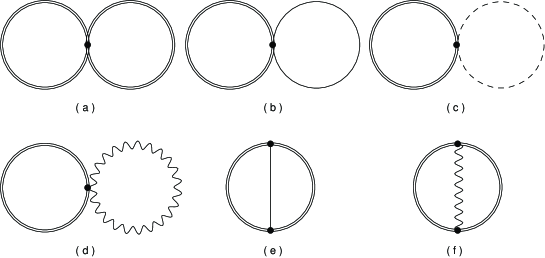
Figure 2: Diagram $(a)$ contributes to leading and subleading orders, while the other diagrams are of subleading order in the large $N$ expansion.

plus the one-loop contribution that come from the trace of the superdeterminants of the complex superfields, plus a two-loop contribution that comes from the diagram Figure2(a). The traces of superdeterminants are given by:

$$\Gamma_{1loop} = \dfrac{i}{2}(N-1)\mathrm{Tr}\ln[D^{2}+M_{0}]+\dfrac{i}{2}\mathrm{Tr}\ln[D^{2}+M_{1}]$$ (7)

$$+\dfrac{i}{2}\mathrm{Tr}\ln[D^{2}+M_{2}]+\dfrac{i}{2}\mathrm{Tr}\ln[D^{2}+\alpha M_{A}]$$

$$+ \dfrac{i}{2}\mathrm{Tr}\ln\left[-\dfrac{i}{2}\left(1-\dfrac{1}{\alpha}\right){\partial^{\beta}}_{\alpha}+\dfrac{{C^{\beta}}_{\alpha}}{2}\left(1+\dfrac{1}{\alpha}\right)D^{2}+{C^{\beta}}_{\alpha}M_{A}\right].$$

Proceeding as described in Ferrari:2009zx , this one-loop contribution to the effective action can be written:

$$\Gamma_{1loop} = \dfrac{1}{16\pi}\int{d^{5}z}\Big{\{}(N-1)\left[\lambda\sigma_{cl}^{2}\right]^{2}+\left[3\lambda\sigma_{cl}^{2}\right]^{2}+|\lambda\sigma_{cl}^{2}-\alpha\dfrac{g^{2}\sigma_{cl}^{2}}{4}|^{2}$$ (8)

$$+\left[\dfrac{g^{2}\sigma_{cl}^{2}}{2}\right]^{2}+\left[\alpha\dfrac{g^{2}\sigma_{cl}^{2}}{2}\right]^{2}\Big{\}}.$$

The two-loop contributions, drawn in Figure2, are given by

$$\Gamma_{2loop} = \int{d^{5}z}\Big{\{}(N+2)\dfrac{\lambda^{3}}{16\pi}+\dfrac{\lambda}{16\pi}|\lambda||\lambda+\dfrac{\alpha}{2}g^{2}|-\dfrac{1}{64\pi^{2}}g^{4}|\lambda|\left(1+\alpha|\alpha|\right)$$ (9)

$$+\dfrac{g^{2}}{64\pi^{2}}\left[C_{2}(\epsilon,\lambda,g)+\left(2\lambda^{2}(1+\alpha)+\dfrac{g^{4}}{16}(3-\alpha^{2})-\alpha^{2}\lambda g^{2}\right)\ln\left(\dfrac{\sigma_{cl}^{2}}{\mu}\right)\right]$$

$$-\dfrac{\lambda^{3}}{2\pi^{2}}\left[C_{1}(\epsilon,\lambda)+\ln\left(\dfrac{\sigma_{cl}^{2}}{\mu}\right)\right]\Big{\}}\sigma_{cl}^{4},$$

where

$$C_{1}(\epsilon,\lambda) = -\dfrac{1}{2}\left[\dfrac{1}{\epsilon}-\gamma+1-\ln\left(\dfrac{25\lambda^{2}}{4\pi}\right)\right],$$

$$C_{2}(\epsilon,\lambda,g) = \dfrac{1}{8}\Big{\{}6|\lambda|g^{2}(1+\alpha|\alpha|)-2\lambda^{2}(3-\alpha)+2\left(8\lambda^{2}+\dfrac{3}{4}g^{4}\right)\ln\left(\dfrac{g^{2}+4|\lambda|}{2}\right)$$ (10)

$$+\left(\dfrac{1}{\epsilon}-\gamma+\ln{4\pi}+1\right)\left[8\lambda^{2}(1+\alpha)+\dfrac{g^{4}}{4}(3-\alpha^{3})-4\alpha^{2}\lambda g^{2}\right]$$

$$-2\alpha\left(8\lambda^{2}-4\alpha\lambda g^{2}-\dfrac{\alpha^{2}}{4}g^{4}\right)\ln\left(\dfrac{g^{2}+4|\lambda|}{2}\right)\Big{\}}.$$

The integrals were evaluated using the regularization by dimensional reduction Siegel:1979wq . In three dimensions this regularization scheme avoids any divergence at one-loop level, and so, no mass renormalization is necessary.

The effective action at subleading order is obtained by adding Eqs. (6), (8) and (9) and can be cast as

$$\Gamma = \int{d^{5}z}\Big{\{}N\frac{\lambda}{4}+(N+8)\frac{\lambda^{2}}{16\pi}+\frac{1}{16\pi}|\lambda-\alpha\frac{g^{2}}{4}|^{2}+(1+4\alpha^{2})\frac{g^{4}}{256\pi}$$ (11)

$$+(N+2)\dfrac{\lambda^{3}}{16\pi^{2}}+\dfrac{\lambda}{16\pi^{2}}|\lambda||\lambda+\dfrac{\alpha}{2}g^{2}|-\dfrac{1}{64\pi^{2}}g^{4}|\lambda|\left(1+\alpha|\alpha|\right)$$

$$+\dfrac{g^{2}}{64\pi^{2}}\left[C_{2}(\epsilon,\lambda,g)+\left(2\lambda^{2}(1+\alpha)+\dfrac{g^{4}}{16}(3-\alpha^{2})-\alpha^{2}\lambda g^{2}\right)\ln\left(\dfrac{\sigma_{cl}^{2}}{\mu}\right)\right]$$

$$-\dfrac{\lambda^{3}}{2\pi^{2}}\left[C_{1}(\epsilon,\lambda)+\ln\left(\dfrac{\sigma_{cl}^{2}}{\mu}\right)\right]+B\sigma_{cl}^{4}\Big{\}}\sigma_{cl}^{4}$$

$$= -\int{d^{5}z}\leavevmode\nobreak\ K_{eff},$$

where $K_{eff}$ is the Kählerian effective superpotential; $B$ is a convenient counterterm to renormalize the model. It is well known that the effective (super) potential is a gauge-dependent quantity Jackiw:1974cv .

Following the renormalization procedure as described in Coleman:1973jx , and observing that divergences larger than logarithmic does not show up, which constrains the mass counterterm to be trivial, the only necessary condition to renormalize the ${\cal{N}}=1$ $SCSM$ model can be cast as

$$\dfrac{\partial^{4}K_{eff}}{\partial\sigma_{cl}^{4}}\Big{|}_{\sigma_{cl}=v}=-4!\dfrac{N\lambda}{4}\leavevmode\nobreak\ ,$$ (12)

where $v$ is a mass scale independent of the Grassmanian coordinate $\theta$. This feature means that we are evaluating the derivatives on $K_{eff}$ at $\sigma_{cl}=\sigma_{1}=v$.

We determine $B$ by solving the Eq.(12). Substituting the result in Eq.(11) we obtain the following expression for the Kählerian effective superpotential

$$K_{eff} = -N\dfrac{\lambda}{4}\sigma_{cl}^{4}+\dfrac{e}{1024\pi^{2}}\sigma_{cl}^{4}\left[-\dfrac{25}{6}+\ln\dfrac{\sigma_{cl}^{2}}{v^{2}}\right],$$ (13)

where

$$e=(\alpha^{2}-3)g^{6}+16\alpha^{2}g^{4}\lambda-32(\alpha+1)g^{2}\lambda^{2}+512\lambda^{3}.$$ (14)

The renormalization of $K_{eff}$ requires the introduction of the mass scale, $v$, at sub-leading order in $1/N$, dynamically breaking the superconformal invariance of the model.

To analyze the possibility of a dynamical breaking of the gauge symmetry we have to determine if the superfield $\sigma_{cl}$ acquires a non-vanishing vacuum expectation value (VEV). For this we must determine the conditions for the minimum of the effective scalar potential $V_{eff}=\int{d^{2}\theta}K_{eff}$. So, after integrating over the Grassmaniann coordinates, $V_{eff}$ can be cast as

$$V_{eff}=-N\lambda\sigma_{2}\sigma_{1}^{3}+\dfrac{e}{512\pi^{2}}\sigma_{2}\sigma_{1}^{3}\left[-\dfrac{22}{3}+\ln{\dfrac{\sigma_{1}}{v}}\right]\leavevmode\nobreak\ .$$ (15)

The conditions that minimize $V_{eff}$ are

$$\dfrac{\partial V_{eff}}{\partial\sigma_{1}} = 3\sigma_{2}\sigma_{1}^{2}\left[-N\lambda+\dfrac{e}{512\pi^{2}}\left(-\dfrac{19}{3}+\ln\dfrac{\sigma_{1}}{v}\right)\right]=0\leavevmode\nobreak\ ,$$ (16)

$$\dfrac{\partial V_{eff}}{\partial\sigma_{2}} = \sigma_{1}^{3}\left[-N\lambda+\dfrac{e}{512\pi^{2}}\left(-\dfrac{22}{3}+\ln\dfrac{\sigma_{1}}{v}\right)\right]=0\leavevmode\nobreak\ .$$ (17)

We can see that $\sigma_{2}=0$ gives a vanishing $V_{eff}$ (supersymmetric vacuum) in the minimum only if Eqs. (16) and (17) are both satisfied. The Eq.(16) is readily satisfied for $\sigma_{2}=0$, and the condition Eq.(17) possesses two solutions:

$$\sigma_{1} = 0\leavevmode\nobreak\ ,$$ (18)

$$\sigma_{1} = v\leavevmode\nobreak\ \exp\Big{\{}\dfrac{11}{6}+\dfrac{128N\pi^{2}\lambda}{e}\Big{\}}.$$ (19)

The first one is the trivial solution, and the complex scalar matter superfield $\Phi_{N}$ does not acquire a non-vanishing VEV. This solution represents a gauge invariant phase. The other solution, Eq.(19), represents a non-vanishing VEV for the superfield $\Phi_{N}$, generating masses for the gauge superfield $\Gamma$, the scalar complex superfield $\Phi_{j}$ and for the real scalar superfield $\Sigma$.

To be consistent with the approximation we used, the minimum of effective potential must lay around $\sigma_{cl}\sim v$, constraining the exponential function to be approximately $1$. Therefore, the coupling $\lambda$ should satisfy

$$\lambda = -\dfrac{11}{48\pi^{2}N}\left[\dfrac{(\alpha^{2}-3)}{16}g^{6}+\alpha^{2}g^{4}\lambda-2(\alpha+1)g^{2}\lambda^{2}+32\lambda^{3}\right].$$ (20)

We can see that in first order the coupling $\lambda$ is very small, of order $1/48N$. This result justifies our choice of studying the model in the $1/N$ approximation and truncating the expansion in powers of $\lambda$. Thus, the dynamical breaking of gauge and superconformal invariances in the ${\cal{N}}=1$ SCSM model is compatible with $1/N$ expansion presented here. The compatibility between $1/N$ expansion of ${\cal{N}}=1$ SCSM model and the Coleman-Weinberg mechanism is not a big surprise, once this effect was shown to be possible in a perturbative approach in the supersymmetric Ferrari:2010ex and non-supersymmetric Dias:2003pw variations of the model, where we have the freedom to play with the two independent gauge and self-interaction coupling constants, as in the original work of Coleman and Weinberg. But here we have a crucial difference. Beyond self-interaction and gauge couplings we have the parameter $N$, doing that no restriction on the order of gauge coupling $g$ be necessary.

III ${\cal{N}}=2$ SUSY Chern-Simons-matter model

One case of interest is the extension of the number of supersymmetries of the SCSM model to ${\cal{N}}=2$ Siegel:1979fr ; Gates:1991qn ; Nishino:1991sr . This step is given just identifying the coupling constants $\lambda=\dfrac{g^{2}}{4}$ to eliminate fermion-number violating terms in the action written in terms of component fields, as discussed in Lee:1990it ; Ivanov:1991fn . Performing this identification and a similar renormalization procedure through a condition like the Eq.(12), the expression of the effective Kählerian superpotential can be cast as

$$K_{eff} = -N\dfrac{g^{2}}{16}\sigma_{cl}^{4}+c(\alpha)\dfrac{g^{6}}{1024\pi^{2}}\sigma_{cl}^{4}\left[-\dfrac{25}{6}+\ln\dfrac{\sigma_{cl}^{2}}{v^{2}}\right],$$ (21)

where $c(\alpha)=[3+\alpha(5\alpha-2)]$ is non-null for any real $\alpha$. So, for the ${\cal{N}}=2$ SCSM model, the scalar effective potential $V_{eff}$ is given by

$$V_{eff2}=-N\frac{g^{2}}{4}\sigma_{2}\sigma_{1}^{3}+c(\alpha)\dfrac{g^{6}}{512\pi^{2}}\sigma_{2}\sigma_{1}^{3}\left[-\dfrac{22}{3}+\ln{\dfrac{\sigma_{1}}{v}}\right]\leavevmode\nobreak\ .$$ (22)

Just as for ${\cal{N}}=1$ case, the conditions that minimize $V_{eff2}$ are

$$\dfrac{\partial V_{eff2}}{\partial\sigma_{1}} = 3g^{2}\sigma_{2}\sigma_{1}^{2}\left[-\frac{N}{4}+c(\alpha)\dfrac{g^{4}}{512\pi^{2}}\left(-\dfrac{19}{3}+\ln\dfrac{\sigma_{1}}{v}\right)\right]=0\leavevmode\nobreak\ ,$$ (23)

$$\dfrac{\partial V_{eff2}}{\partial\sigma_{2}} = g^{2}\sigma_{1}^{3}\left[-\frac{N}{4}+c(\alpha)\dfrac{g^{4}}{512\pi^{2}}\left(-\dfrac{22}{3}+\ln\dfrac{\sigma_{1}}{v}\right)\right]=0\leavevmode\nobreak\ .$$ (24)

Again $\sigma_{2}=0$ gives a vanishing $V_{eff2}$ in the minimum only if Eqs. (23) and (24) are satisfied. Once $\sigma_{2}=0$ is the supersymmetric solution, we just have to compute the solution of Eq.(24), that are given by:

$$\sigma_{1} = 0\leavevmode\nobreak\ ,$$ (25)

$$\sigma_{1} = v\leavevmode\nobreak\ \exp\Big{\{}\dfrac{11}{6}+\dfrac{32N\pi^{2}}{c(\alpha)g^{4}}\Big{\}}.$$ (26)

Of course, $\sigma_{1}=0$ is the gauge symmetric solution just like ${\cal{N}}=1$ case. For the second solution, if the minimum of effective superpotential lies around $\sigma_{cl}\sim v$, the coupling $g$ should satisfy

$$\dfrac{g^{4}}{N}=-\dfrac{192\pi^{2}}{11c(\alpha)}\approx-\frac{172}{c(\alpha)}\leavevmode\nobreak\ ,$$ (27)

This fact determines $g$ to be of the order of $\left(\dfrac{N}{c(\alpha)}\right)^{1/4}$. If we observe that in the classical action every time that the coupling constant $g$ appears it is accompanied of a factor $1/\sqrt{N}$, we can see that we have an effective coupling of the order of $1/N^{1/4}$. But, the trilinear terms proportional to $\lambda/\sqrt{N}$, when we lift from ${\cal{N}}=1$ to ${\cal{N}}=2$, will be of order of $\lambda/\sqrt{N}\rightarrow-g^{2}/2\sqrt{N}\approx-1/2$. Therefore, our $1/N$ expansion loses its sense. This situation is similar to what happens in the perturbative (loop) expansion, where the Coleman-Weinberg mechanism for the ${\cal{N}}=2$ SCSM model is not compatible with perturbation theory Ferrari:2010ex . This result is in agreement with previous works Gaiotto:2007qi ; Buchbinder:2009dc ; Buchbinder:2010em , where several aspects of $N=2,3$ SCSM models were studied. Moreover, the above condition constrains $g^{2}$ to be imaginary, compromising the unitarity of the theory.

IV Concluding remarks

Summarizing, in this Letter we studied the spontaneous breaking of the superconformal and gauge invariances in the three-dimensional Abelian ${\cal{N}}=1,2$ SCSM theories in the large $N$ limit approximation. It is shown that the dynamical breaking of superconformal and gauge invariances in the ${\cal{N}}=1$ SCSM model is compatible with $1/N$ expansion, if the matter self-interaction coupling constant $\lambda$ is of the order of $g^{6}/N$, while no restriction to the order of gauge coupling $g$ has to be imposed. In the ${\cal{N}}=2$ extension of SCSM model it is observed that as in the perturbative approach, the Coleman-Weinberg mechanism is not possible in the $1/N$ expansion, due to the constraint between the coupling constants. It is expected that non-Abelian extensions of the SCSM model share the same properties discussed here, once that the presence of logarithmic divergent Feynman diagrams of two-loop contributions that appear at subleading order in the $1/N$ expansion will also be present in such extensions.

Acknowledgments. This work was partially supported by the Brazilian agencies Conselho Nacional de Desenvolvimento Científico e Tecnológico (CNPq) and Fundação de Amparo à Pesquisa do Estado de São Paulo (FAPESP).

References

- (1) J. M. Maldacena, Adv. Theor. Math. Phys. 2, 231 (1998) [Int. J. Theor. Phys. 38, 1113 (1999)].
- (2) S. S. Gubser, I. R. Klebanov and A. M. Polyakov, Phys. Lett. B 428, 105 (1998).
- (3) E. Witten, Adv. Theor. Math. Phys. 2, 253 (1998).
- (4) R. A. Janik and R. B. Peschanski, Phys. Rev. D 73, 045013 (2006); C. P. Herzog, P. K. Kovtun and D. T. Son, Phys. Rev. D 79, 066002 (2009); C. P. Herzog and A. Yarom, Phys. Rev. D 80, 106002 (2009).
- (5) S. A. Hartnoll, C. P. Herzog and G. T. Horowitz, Phys. Rev. D 80, 106002 (2009); S. S. Gubser, C. P. Herzog, S. S. Pufu and T. Tesileanu, Phys. Rev. Lett. 103, 141601 (2009).
- (6) F. Aprile, S. Franco, D. Rodriguez-Gomez and J. G. Russo, JHEP 1005, 102 (2010).
- (7) D. Gaiotto and X. Yin, JHEP 0708, 056 (2007).
- (8) J. Bagger and N. Lambert, Phys. Rev. D 75, 045020 (2007); Phys. Rev. D 77, 065008 (2008).
- (9) C. Krishnan and C. Maccaferri, JHEP 0807, 005 (2008).
- (10) A. Gustavsson, Nucl. Phys. B 811, 66 (2009).
- (11) A. G. Dias, M. Gomes and A. J. da Silva, Phys. Rev. D 69, 065011 (2004).
- (12) S. R. Coleman and E. Weinberg, Phys. Rev. D 7, 1888 (1973).
- (13) A. F. Ferrari, E. A. Gallegos, M. Gomes, A. C. Lehum, J. R. Nascimento, A. Y. Petrov and A. J. da Silva, Phys. Rev. D 82, 025002 (2010).
- (14) S. J. Gates, M. T. Grisaru, M. Rocek and W. Siegel, Front. Phys. 58, 1 (1983).
- (15) A. C. Lehum, A. F. Ferrari, M. Gomes and A. J. da Silva, Phys. Rev. D 76, 105021 (2007).
- (16) C. P. Burgess, Nucl. Phys. B 216, 459 (1983).
- (17) A. F. Ferrari, M. Gomes, A. C. Lehum, J. R. Nascimento, A. Y. Petrov, E. O. Silva and A. J. da Silva, Phys. Lett. B 678, 500 (2009).
- (18) A. C. Lehum, Phys. Rev. D 77, 067701 (2008).
- (19) W. Siegel, Phys. Lett. B 84, 193 (1979).
- (20) R. Jackiw, Phys. Rev. D 9, 1686 (1974).
- (21) W. Siegel, Nucl. Phys. B 156, 135 (1979).
- (22) S. J. J. Gates and H. Nishino, Phys. Lett. B 281, 72 (1992).
- (23) H. Nishino and S. J. J. Gates, Int. J. Mod. Phys. A 8, 3371 (1993).
- (24) C. K. Lee, K. M. Lee and E. J. Weinberg, Phys. Lett. B 243, 105 (1990).
- (25) E. A. Ivanov, Phys. Lett. B 268, 203 (1991).
- (26) I. L. Buchbinder, E. A. Ivanov, O. Lechtenfeld, N. G. Pletnev, I. B. Samsonov and B. M. Zupnik, JHEP 0910, 075 (2009).
- (27) I. L. Buchbinder, N. G. Pletnev and I. B. Samsonov, JHEP 1004, 124 (2010).