Multi-frequency, thermally coupled radiative transfer with TRAPHIC: Method and tests

Abstract

We present an extension of traphic, the method for radiative transfer of ionising radiation in smoothed particle hydrodynamics simulations that we introduced in Pawlik & Schaye (2008). The new version keeps all advantages of the original implementation: photons are transported at the speed of light, in a photon-conserving manner, directly on the spatially adaptive, unstructured grid traced out by the particles, in a computation time that is independent of the number of radiation sources, and in parallel on distributed memory machines. We extend the method to include multiple frequencies, both hydrogen and helium, and to model the coupled evolution of the temperature and ionisation balance. We test our methods by performing a set of simulations of increasing complexity and including a small cosmological reionisation run. The results are in excellent agreement with exact solutions, where available, and also with results obtained with other codes if we make similar assumptions and account for differences in the atomic rates used. We use the new implementation to illustrate the differences between simulations that compute photoheating in the grey approximation and those that use multiple frequency bins. We show that close to ionising sources the grey approximation asymptotes to the multi-frequency result if photoheating rates are computed in the optically thin limit, but that the grey approximation breaks down everywhere if, as is often done, the optically thick limit is assumed.

1 Introduction

New telescopes such as Planck, LOFAR, MWA, ALMA and JWST will soon open up new windows onto the epoch of reionisation (e.g., Barkana & Loeb, 2001; Ciardi & Ferrara, 2005; Fan, Carilli, & Keating, 2006; Furlanetto, Oh, & Briggs, 2006 for reviews of this epoch). Data collected by these telescopes is expected to shed light on many unresolved issues in our current understanding of how galaxies form and evolve and interact with their surroundings. Detailed theoretical studies, however, will be needed to interpret it. Amongst the most promising techniques to perform such studies are cosmological simulations of reionisation.

Modern simulations of reionisation aim to combine the first-principle modelling of the gravitational growth of density fluctuations and of the hydrodynamical evolution of the cosmic gas in the expanding Universe with recipes for star formation and associated feedback and to follow also the propagation of ionising radiation emitted by the first ionising sources. The computationally efficient, but accurate implementation of the radiative transfer (RT) is currently one of the biggest challenges for simulating reionisation.

Computing the ionising intensity throughout the simulation box requires solving the seven-dimensional (three space coordinates, two directional coordinates, frequency and time) RT equation. This is a formidable task, not only because of the high dimensionality of the problem, but also because of the large number of ionising sources contained in typical cosmological volumes. To accomplish it, existing approaches (e.g., Abel, Norman, & Madau, 1999; Gnedin & Abel, 2001; Ciardi et al., 2001; Nakamoto, Umemura, & Susa, 2001; Maselli, Ferrara, & Ciardi, 2003; Razoumov & Cardall, 2005; Mellema et al., 2006; Susa, 2006; Ritzerveld & Icke, 2006; McQuinn et al., 2007; Semelin, Combes, & Baek, 2007; Trac & Cen, 2007; Pawlik & Schaye, 2008; Aubert & Teyssier, 2008; Altay, Croft, & Pelupessy, 2008; Petkova & Springel, 2009; Finlator, Özel, & Davé, 2009; Gritschneder et al., 2009; Paardekooper, Kruip, & Icke, 2010; Hasegawa & Umemura, 2010; Cantalupo & Porciani, 2010; Partl et al., 2010) to transport ionising photons must often resort to a number of approximations.

The accuracy of several ionising (cosmological) RT codes has been assessed in test simulations that were performed as part of a series of comparison projects (Iliev et al., 2006a; Iliev et al., 2009). The results of the comparisons are encouraging and indicate that the participating codes have reached a certain level of maturity (Iliev et al., 2009). The design of most of the test simulations was kept simple in order to facilitate comparisons between different RT codes. More recently, the performance of different RT codes has been compared in cosmological simulations of reionisation with an equally promising degree of agreement (Zahn et al., 2010). However, the inclusion of RT in state-of-the-art simulations of structure formation remains a tough computational challenge, as we now explain.

RT codes that are both spatially adaptive and parallel on distributed memory are still rare (see, e.g., Table 1 in Iliev et al., 2006a and Table 1 in Iliev et al., 2009). Nearly all reionisation simulations are therefore performed on uniform grids. Combined with the fact that large simulation boxes are needed to model representative volumes of the Universe, this means that the spatial resolution of state-of-the-art RT simulations of reionisation is typically far below that of the underlying spatially adaptive hydrodynamical simulations. In fact, many RT simulations of reionisation ignore hydrodynamical effects altogether and assume the gas traces the dark matter. Small-scale structure in the cosmic gas is therefore often ignored or included only in a statistically sense.

Cosmological simulations of reionisation typically contain millions of star particles (e.g., Iliev et al., 2006b). Large numbers of ionising sources pose a challenge to simulations of reionisation because for most of the existing RT methods the computation times increases linearly with the source number. The usual practice of reducing the number of ionising sources by combining sources that fall into the same cell of a superimposed mesh renders reionisation simulations feasible, but also reduces the spatial resolution at which the RT is performed. Note that the inclusion of diffuse ionising radiation emitted by recombining ions further increases the number of ionising sources. To reduce the computational effort, this recombination radiation is therefore usually treated using the on-the-spot approximation (e.g., Osterbrock, 1989), which assumes it to be re-absorbed in the immediate vicinity of the recombining ion. However, the validity of this approximation remains to be assessed (e.g., Ritzerveld, 2005; Williams & Henney, 2009, Hasegawa & Umemura, 2010).

RT simulations of reionisation are still often performed by post-processing pre-computed static density fields. This static approximation is appropriate for simulating the initial phase of rapid growth of ionised regions or the propagation of ionisation fronts on cosmological scales (see, e.g., the discussion in Iliev et al., 2006b). Once the speed of ionisation fronts becomes comparable to the sound speed of the ionised gas, the static approximation, however, becomes inapplicable and a full radiation-hydrodynamical treatment is required. In any case, the static approximation breaks down after about a sound-crossing time, as the Jeans filtering of the gas can then no longer be ignored (e.g., Gnedin, 2000). Although radiation-hydrodynamical feedback from reionisation is known to play a key role, most of the large-scale reionisation simulations performed to date ignore it.

In Pawlik & Schaye (2008, hereafter Paper I) we presented the RT method traphic (TRAnsport of PHotons In Cones) for use in Smoothed Particle Hydrodynamics (SPH; Gingold & Monaghan, 1977; Lucy, 1977) simulations. traphic can be used to solve both the time-independent and the time-dependent RT equation in an explicitly photon-conserving manner. It employs the full spatial resolution of the underlying SPH simulation because it works directly on the unstructured grid formed by the discrete set of SPH particles. It achieves directed transport of radiation on the irregular distribution of SPH particles by tracing photon packets inside cones. The solid angle of these cones thereby sets the angular resolution at which the RT is performed. traphic is by construction parallel on distributed memory machines if the SPH simulation itself is parallel on distributed memory machines.

The computational cost for simulations with traphic is independent of the number of ionising sources. It merely scales with the product of the number of spatial and angular resolution elements, i.e. with the number of SPH particles and the number of cones needed to tessellate the sky. For comparison, the computational cost of conventional ray and photon tracing methods scales with the product of the number of spatial resolution elements (gas particles or gas cells) and the number of sources. Since the number of sources is typically proportional to the number of spatial resolution elements, conventional ray and photon tracing methods face an expensive scaling with the square of the number of spatial resolution elements. In contrast, a relatively small number of angular resolution elements is typically sufficient to obtain converged results (Paper I; see also, e.g., Trac & Cen, 2007; Paardekooper, Kruip, & Icke, 2010), and this, in combination with the independence of the computational cost of the source number, makes traphic ideal for simulations containing large numbers of sources (as is the case for, e.g., reionisation simulations) as well as for an explicit treatment of the diffuse radiation component.

In Paper I we presented an implementation of traphic for use on (sets of) static density fields in the SPH code gadget (Springel, 2005). We applied this implementation to the transport of monochromatic ionising radiation in hydrogen-only gas at a fixed temperature. We demonstrated its excellent performance in several (static density field) test problems that were designed to allow a detailed comparison to results obtained with other RT codes. Here we describe, test and discuss an extension of this implementation. The new implementation of traphic allows for the transport of multi-frequency radiation in primordial gas, i.e., in gas consisting of both hydrogen and helium. In addition to the computation of the ionisation state, it also allows for the self-consistent computation of the temperature of photoionised gas. The new implementation still solves the RT equation only on static density fields. The radiation-hydrodynamical coupling of traphic will be described in a future work.

Because the computational cost for RT simulations is typically proportional to the number of frequencies at which the RT equation is solved, many RT simulations of ionising radiation discretize the RT problem using only a single frequency bin. In the grey approximation (e.g., Mihalas & Weibel Mihalas, 1984), ionising radiation within this bin is then assigned an effective absorption cross-section and an effective photoenergy that is injected in the gas upon absorption (for examples see, e.g., Iliev et al., 2006a). The corresponding photoionisation heating rates can be computed assuming the optically thin or the optically thick limit. We use our new implementation to show that RT simulations which employ the grey approximation yield gas temperatures that agree with the exact multi-frequency solution only if grey photoheating rates are computed in the optically thin limit and then only close to the ionising sources. Grey RT simulations that compute photoheating rates in the optically thick limit significantly overestimate the typical temperatures of the photo-heated gas. A related treatment of this subject and a discussion of its astrophysical implications can be found in Abel & Haehnelt (1999).

The structure of this paper is as follows. In Sec. 2 we present a brief review of the main concepts behind traphic. In Sec. 3 we then discuss the equations that govern the evolution of the ionisation state and temperature of gas exposed to ionising radiation. With these preparations in hand we are ready to present our new implementation of traphic in Sec. 4 (and in the appendix). We discuss an extensive set of tests of this implementation (on static density fields) in Sec. 5. There we also investigate the applicability of the grey approximation by comparing simulations using the grey approximation with simulations using multiple frequency bins. We conclude with a brief summary in Sec. 6.

2 TRAnsport of PHotons In Cones

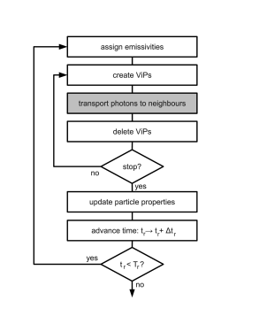
Figure 1: Flow charts. Left chart: overview of traphic. The RT simulation starts with the assignment of emissivities to source particles. Thereafter, photon packets are transported from all particles to their neighbours (see right chart for details). ViPs, if needed, are created in advance of the transport and are deleted immediately afterwards. The transport cycle continues until the user-defined stopping criterion is satisfied. Then, the properties of the particles are updated according to the photon-gas interactions that occurred. Finally, the RT time step is advanced. The RT simulation ends at time $T_{\rm r}$. Right chart: details of the transport of photons to neighbours (grey box in the left chart). Photons in photon packets are distribute amongst the $\tilde{N}_{\rm ngb}$ neighbouring particles inside $N_{\rm c}$ (tessellating) emission or (regular) transmission cones with solid angle $4\pi/N_{\rm c}$ centred on the corresponding propagation directions. The optical depth to each neighbour is computed and the fraction of transmitted and absorbed/scattered photons is determined. Multiple photon packets received by individual neighbours are merged in $N_{\rm c}$ (tessellating) reception cones separately for each frequency $\nu$, which limits the number of photon packets stored at each particle to at most $N_{\rm c}\times N_{\nu}$.

In this section we briefly summarise the basic concepts underlying the RT method traphic and introduce some of the notation that will be frequently employed in the following sections. The reader is referred to the original description in Sec. 4 of Paper I for more details as that description remains valid. The extensions presented in this work concern only the application of traphic to the transport of ionising photons, which will be described in Sec. 4.

To introduce essential notation we briefly recall that SPH is a Lagrangian numerical method to solve the Euler equations of fluid dynamics through the representation of continuum fluids by discrete sets of particles (for reviews see, e.g., Monaghan, 2005; Springel, 2010). Any property, say $A_{i}$, of any given particle $i$ is determined by performing a weighted average, or smoothing, $A_{i}=\sum_{j}m_{j}/\rho_{j}A_{j}W_{ij}(h)$ of the corresponding property $A_{j}$ of all other particles $j$, where $m_{j}$ and $\rho_{j}$ are the mass and density of particle $j$, and $W_{ij}(h)$ is the SPH kernel that depends on the SPH smoothing length $h$.

In the following we make the common assumption that the kernel $W_{ij}$ is compact so that there is a finite number $N_{\rm ngb}$ of neighbouring particles $j$ within a sphere of radius $h$ around particle $i$. If the smoothing lengths, which represent the spatial resolution elements of the SPH simulation, are allowed to vary in space such that the number of neighbours $N_{\rm ngb}$ remains fixed, then SPH enables simulations whose spatial resolution adapts to the fluid geometry. It is this feature that makes simulations with a large dynamic range possible and that is perhaps the main reason for the numerous and successful applications of SPH to solve multi-scale astrophysical problems such as galaxy formation and reionisation.

traphic transports photons directly on the SPH particles (i.e. without interpolation to a superimposed numerical grid) and hence the full dynamic range of the SPH simulation is employed. The photon transport can be decomposed into the emission of photon packets by source particles followed by their directed propagation on the irregular set of SPH particles. We now briefly describe both these parts in turn.

Photon packets, each of which carries photons of a characteristic frequency $\nu$, are emitted from source particles to their $\tilde{N}_{\rm ngb}$ neighbouring SPH particles (residing in a sphere of radius $\tilde{h}$ centred on the source) using a tessellating set of $N_{\rm c}$ emission cones. The number of neighbours $\tilde{N}_{\rm ngb}$ is a parameter that determines the spatial resolution and is usually matched to the number of neighbours $N_{\rm ngb}$ (residing in the sphere of radius $h$) used in the computation of the SPH particle properties, i.e., $\tilde{N}_{\rm ngb}\lesssim N_{\rm ngb}$. The number of cones $N_{\rm c}$ is a parameter that determines the angular resolution of the RT. Emission cones are necessary to achieve an isotropic emission despite the generally highly irregular distribution of SPH particles (see App. A in Paper I). The last parameter that controls the emission of photon packets by source particles is the number $N_{\nu}$ of frequency bins that are used to discretize the associated radiation spectrum.

Each of the emitted photon packets (of frequency $\nu$) has an associated propagation direction. This propagation direction is chosen to be parallel to the central axis of the corresponding emission cone. After emission, the photon packets are traced downstream along their propagation directions. The packets thereby remain confined to the solid angle of the emission cone into which they were originally emitted thanks to the use of transmission cones with solid angle $4\pi/N_{\rm c}$. The transmission cones prevent the unconfined diffusion of photon packets on the unstructured grid of SPH particles that would otherwise occur and they ensure that the transport is directed. Because the transmission cones are defined locally (i.e., at the positions of the transmitting particles) and because photon packets are only transmitted to the subset of the $\tilde{N}_{\rm ngb}$ nearest neighbours that are inside the transmission cones, the angular resolution at which photon packets are transferred is independent of the distance from the source (even though the surface areas implied by the solid angles of the original emission cones increase with the square of the distances from the corresponding sources). As a result, the sharpness of the shadows cast by opaque objects such as dense neutral clumps and filaments is independent of their distances from the sources.

Virtual particles (ViPs) are introduced to accomplish the photon transport along directions for which no neighbouring SPH particle in the associated emission or transmission cones could be found. The properties of the ViPs (like, e.g., their densities) are determined through SPH interpolation from the $\tilde{N}_{\rm ngb}$ neighbouring SPH particles. Their name refers to the fact that ViPs are temporary constructs that are only invoked to accomplish the transport of photon packets in empty cones. They do not hold permanent information, they do not affect the SPH simulation and they are deleted as soon as they have fulfilled this task.

The photon transport is supplemented with a photon packet merging procedure that respects the chosen angular resolution and renders the RT computation time independent of the source number. The merging is done by binning photon packets in angle (according to their propagation directions) using $N_{\rm c}$ (tessellating) reception cones. Binned photon packets define a single new photon packet per reception cone whose propagation direction is given by the weighted sum of the propagation directions of photon packets received in that cone. The merging is done separately for photon packets of different frequencies. Thus, it does not change the mean free path of the photon packets, which is important for simulations that contain radiation sources with a broad range of spectral properties (e.g., quasars and stellar sources). Thanks to the merging, at each particle at most $N_{\rm c}\times N_{\nu}$ photons packets need to be stored.

The photon transport is performed using RT time steps $\Delta t_{\rm r}$ (see Sec. 5.2.3 in Paper I for a detailed discussion of the size of time steps in reionisation simulations). During each such time step, photons are propagated and their interactions with the gas are computed until a certain stopping criterion is satisfied. The criterion depends on whether one aims to solve the time-independent or the time-dependent RT equation. In the first case, photons are propagated until they are absorbed or have left the computational domain. In the second case, photon clocks associated with each photon packet are used to synchronise the packet’s travel time with the simulation time such that photon packets travel at the speed of light.

After each time step, the state of the SPH particles is updated according to the interactions (absorptions, scatterings) with photon packets they experienced. In Sec. 4 we will explain, for the example of absorption of ionising radiation, how to combine the photon transport discussed here with the evaluation of the interactions according to the optical depth encountered by photon packets. Finally, the RT time is advanced, which concludes the algorithm. A schematic summary of the RT method is depicted in the flow chart in Fig. 1.

3 Ionising photons in primordial gas: theory

In this section we outline the physical processes that determine the evolution of the ionisation state (Sec. 3.1) and temperature (Sec. 3.2) of primordial gas exposed to ionising radiation. We discuss the underlying equations and present the references to atomic data required to evaluate them. The description of the numerical implementation used to solve these equations is deferred to Sec. 4.

Readers familiar with the physics of ionisation, recombination, heating and cooling may wish to skip Secs. 3.1 and 3.2 and refer to them only when needed. For those readers we have summarised the physical processes that we include in the computations of the ionisation and thermal state of gas in the RT simulations presented later in this work, together with the references to the (fits to) atomic data sets employed for their numerical evaluation, in Table 1. A detailed discussion of our choice for certain (fits to) atomic data sets and a comparison with other works can be found in Pawlik (2009).

We start with some definitions that we will employ throughout the rest of this work. We consider an atomic gas of total number density $n=n_{\rm e}+\sum n_{\alpha}$, where $n_{\alpha}$ is the number density of species $\alpha$ and $n_{\rm e}$ is the number density of free electrons. The number density $n_{\alpha}$ is related to the total mass density $\rho$ through $n_{\alpha}=X_{\alpha}\rho/(\mu_{\alpha}m_{\rm H})$, where $X_{\alpha}$ is the mass fraction of species $\alpha$ and $\mu_{\alpha}=m_{\alpha}/m_{\rm H}$ is its mass $m_{\alpha}$ in units of the hydrogen mass $m_{\rm H}$. We assume that the gas is of primordial composition, i.e. $\alpha\in\{\rm HI$, $\rm HII$, $\rm HeI$, $\rm HeII$, $\rm HeIII\}$ and $X_{\rm H}+X_{\rm He}=1$. We will set $X_{\rm H}=0.25$. We will make frequent use of the species number density fractions with respect to the hydrogen number density, $\eta_{\alpha}\equiv n_{\alpha}/n_{\rm H}$ and the electron fraction $\eta_{\rm e}=n_{\rm e}/n_{\rm H}$.

3.1 Ionisation and recombination

The evolution of the ionisation state of primordial gas in the presence of a photoionising radiation background of mean intensity $J_{\nu}(\nu)$ is determined by the set of rate equations

$$\frac{d\eta_{\rm HI}}{dt} = \alpha_{\rm HII}n_{\rm e}\eta_{\rm HII}-\eta_{\rm HI}(\Gamma_{\gamma\rm HI}+\Gamma_{\rm eHI}n_{\rm e})$$ (1)

$$\frac{d\eta_{\rm HeI}}{dt} = \alpha_{\rm HeII}n_{\rm e}\eta_{\rm HeII}-\eta_{\rm HeI}(\Gamma_{\gamma\rm HeI}+\Gamma_{\rm eHeI}n_{\rm e})$$ (2)

$$\frac{d\eta_{\rm HeIII}}{dt} = \eta_{\rm HeII}(\Gamma_{\gamma\rm HeII}+\Gamma_{\rm eHeII}n_{\rm e})-\alpha_{\rm HeIII}n_{\rm e}\eta_{\rm HeIII},$$ (3)

supplemented with the closure relations

$$\eta_{\rm HI}+\eta_{\rm HII} = 1$$ (4)

$$\eta_{\rm HeI}+\eta_{\rm HeII}+\eta_{\rm HeIII} = \eta_{\rm He}$$ (5)

$$\eta_{\rm HII}+\eta_{\rm HeII}+2\eta_{\rm HeIII} = \eta_{\rm e},$$ (6)

where $\Gamma_{\gamma\alpha}$ is the photoionisation rate implied by the mean intensity $J_{\nu}$ of the ionising background and $\Gamma_{{\rm e}\alpha}$ and $\alpha_{\alpha}$ are the collisional ionisation and recombination rate coefficients for species $\alpha$; $\eta_{\rm He}\equiv n_{\rm He}/n_{\rm H}=X_{\rm He}(m_{\rm H}/m_{\rm He})/(1-X_{\rm He})$ denotes the helium abundance (by number); $m_{\rm H}$ and $m_{\rm He}$ are the masses of the hydrogen and helium atoms, respectively.

The ionisation and recombination rates are discussed in more detail below.

3.1.1 Ionisation

The photoionisation rate $\Gamma_{\gamma\alpha}$ determines the number of photoionisations of species $\alpha$ per unit time and unit volume $\eta_{\alpha}n_{\rm H}\Gamma_{\gamma\alpha}$. It is defined by (e.g., Osterbrock, 1989)

$$\Gamma_{\gamma\alpha}=\int_{\nu_{\alpha}}^{\infty}~{}d\nu\frac{4\pi J_{\nu}(\nu)}{h_{\rm p}\nu}\sigma_{\gamma\alpha}(\nu),$$ (7)

where $\alpha\in\{\rm HI$, $\rm HeI$, $\rm HeII\}$, $h_{\rm p}$ is Planck’s constant, $\sigma_{\gamma\alpha}(\nu)$ is the photoionisation cross-section and $h_{\rm p}\nu_{\alpha}$ is the ionisation potential. We use the fits to the photoionisation cross-section from Verner et al. (1996). Note that $h_{\rm p}\nu_{\rm HI}=13.6~{}\mbox{eV}$, $h_{\rm p}\nu_{\rm HeI}=24.6~{}\mbox{eV}$ and $h_{\rm p}\nu_{\rm HeII}=54.4~{}\mbox{eV}$.

The photoionisation rates can be written as

$$\Gamma_{\gamma\alpha}=\langle\sigma_{\gamma\alpha}\rangle\int_{\nu_{\alpha}}^{\infty}~{}d\nu\frac{4\pi J_{\nu}(\nu)}{h_{\rm p}\nu},$$ (8)

where $\langle\sigma_{\gamma\alpha}\rangle$ is the average, or grey, photoionisation cross-section,

$$\langle\sigma_{\gamma\alpha}\rangle\equiv\int_{\nu_{\alpha}}^{\infty}~{}d\nu\frac{4\pi J_{\nu}(\nu)}{h_{\rm p}\nu}\sigma_{\gamma\alpha}(\nu)\times\left[\int_{\nu_{\alpha}}^{\infty}~{}d\nu\frac{4\pi J_{\nu}(\nu)}{h_{\rm p}\nu}\right]^{-1}.$$ (9)

We will employ the grey photoionisation cross-section of hydrogen in some of our RT simulations in Sec. 5. For reference we note that its value for a blackbody spectrum of temperature $T_{\rm bb}=10^{5}~{}\mbox{K}$ is $\langle\sigma_{\gamma\rm HI}\rangle=1.63\times 10^{-18}~{}\mbox{cm}^{2}$.

In addition to photoionisations we include collisional ionisation of HI, HeI and HeII by electron impact. To compute the corresponding ionisation rates, we employ the fits to the collisional ionisation coefficients provided by Theuns et al. (1998).

3.1.2 Recombination

We write the number of radiative recombinations per unit time and unit volume of species $\alpha$ (with $\alpha\in\{\rm HII,$ $\rm HeII$, $\rm HeIII\}$) to energy level $l$ of the recombined species as $n_{\rm e}n_{\alpha}\alpha_{\alpha l}$.

Two radiative recombination coefficients are of special interest and are referred to as case A and case B. The case A recombination coefficient $\alpha_{{\rm A}\alpha}\equiv\sum_{l=1}\alpha_{\alpha l}$ is the sum of all the recombination coefficients $\alpha_{\alpha l}$. On the other hand, the case B recombination coefficient is defined as $\alpha_{{\rm B}\alpha}\equiv\sum_{l=2}\alpha_{\alpha l}$ and thus does not include the contribution from recombinations to the ground state.

The introduction of the case B recombination coefficient is motivated by the observation that for pure hydrogen gas that is optically thick to ionising radiation, recombinations to the ground state are cancelled by the immediate re-absorption of the recombination photon by a neutral atom in the vicinity of the recombining ion. RT simulations of ionising radiation in an optically thick hydrogen-only gas may therefore work around the (generally computationally expensive) explicit transfer of recombination photons by simply employing the case B (instead of the full, i.e. case A) recombination coefficient. Note that this on-the-spot approximation (e.g, Osterbrock, 1989) is only strictly valid when considering the transport of ionising radiation in optically thick gas, whereas the gas in RT simulations typically shows a range of optical depths, from optically thick to optically thin.

To keep the description of our method and its test simple and to allow for a detailed comparison with published reference results, we will also assume the on-the-spot approximation and use case B recombination rates. The explicit transport of recombination radiation will be the subject of future work. We use the following coefficients to describe radiative recombinations (Table 1). For HII and HeIII radiative recombination, we employ the fits from Hui & Gnedin (1997). For the HeII radiative recombination coefficient, we employ the tabulated coefficients of Hummer & Storey (1998) using linear interpolation in log-log.

We have not yet discussed the dielectronic contribution to the HeII recombination coefficient. Dielectronic HeII recombination (e.g. Savin, 2000; Badnell, 2001 for a review) is the dominant recombination process for temperatures $T\gtrsim 10^{5}~{}\mbox{K}$. We therefore add the dielectronic contribution to the HeII recombination rates, making use of the fit presented in Aldrovandi & Pequignot (1973).

3.2 Heating and cooling

Our main goal in this work is to present and test an implementation of traphic to compute, in addition to the ionisation state, the evolution of the temperature of gas exposed to ionising radiation. For the discussion it is helpful to review the relevant thermodynamical relations, which is the subject of this section.

The internal energy per unit mass for gas composed of monoatomic species that are at the same temperature $T$ is

$$u=\frac{3}{2}\frac{nk_{\rm B}T}{\rho}=\frac{3}{2}\frac{k_{\rm B}T}{\mu m_{\rm H}},$$ (10)

where $k_{\rm B}$ is the Boltzmann constant and $\mu=\rho/(nm_{\rm H})$ is the mean particle mass in units of the hydrogen mass.

From the first law of thermodynamics

$$d(u\rho V)=-PdV+n_{\rm H}^{2}(\mathcal{H}-\mathcal{C})V,$$ (11)

where $P$ is the pressure, $V$ the volume and $\mathcal{H}$ and $\mathcal{C}$ are the radiative heating and radiative cooling rates, normalised such that the rates of energy gain and loss per unit volume are described by $n_{\rm H}^{2}\mathcal{H}$ and $n_{\rm H}^{2}\mathcal{C}$, respectively. Assuming that $d(\rho V)=0$, as is the case for an SPH particle, it follows that

$$\frac{du}{dt}=-\frac{P}{\rho V}\frac{dV}{dt}+\frac{n_{\rm H}^{2}}{\rho}(\mathcal{H}-\mathcal{C}).$$ (12)

3.2.1 Cooling

The normalised cooling rate $\mathcal{C}$ is the sum of the normalised rates of the individual radiative cooling processes. We include all standard cooling processes: collisional ionisation by electron impact, radiative and dielectronic recombination, collisional excitation by electron impact, bremsstrahlung and Compton scattering. The expressions for the corresponding cooling rates are taken from the references listed in Table 1.

3.2.2 Heating

The normalised heating rate $\mathcal{H}$ is the sum of the rates of the individual radiative heating processes. In the following we only consider the contribution from photoionisation heating, which will be the main contributor to the heating rate for the high-redshift RT simulations of interest. We, however, note that Compton heating by X-rays may not be negligible (Madau & Efstathiou, 1999).

We write the heating rate due to photoionisation as

$$n_{\rm H}^{2}h_{\gamma}=(\eta_{\rm HI}\mathcal{E}_{\gamma\rm HI}+\eta_{\rm HeI}\mathcal{E}_{\gamma\rm HeI}+\eta_{\rm HeII}\mathcal{E}_{\gamma\rm HeII})n_{\rm H},$$ (13)

where

$$\mathcal{E}_{\gamma\alpha}=\int_{\nu_{\alpha}}^{\infty}~{}d\nu\frac{4\pi J_{\nu}(\nu)}{h_{\rm p}\nu}\sigma_{\gamma\alpha}(\nu)(h_{\rm p}\nu-h_{\rm p}\nu_{\alpha})$$ (14)

is the heating rate per particle of species $\alpha$. Using Eq. 7, we can write

$$\mathcal{E}_{\gamma\alpha}=\Gamma_{\gamma\alpha}\langle\epsilon_{\alpha}\rangle,$$ (15)

where

$$\langle\epsilon_{\alpha}\rangle = \left[\int_{\nu_{\alpha}}^{\infty}~{}d\nu\frac{4\pi J_{\nu}(\nu)}{h_{\rm p}\nu}\sigma_{\gamma\alpha}(\nu)(h_{\rm p}\nu-h_{\rm p}\nu_{\alpha})\right]$$ (16)

$$\times \left[\int_{\nu_{\alpha}}^{\infty}~{}d\nu\frac{4\pi J_{\nu}(\nu)}{h_{\rm p}\nu}\sigma_{\gamma\alpha}(\nu)\right]^{-1}$$

is the average excess energy of absorbed ionising photons. For reference, the average excess energy for photoionisation of hydrogen, assuming a blackbody spectrum of temperature $T_{\rm bb}=10^{5}~{}\mbox{K}$, is $\langle\epsilon_{\rm HI}\rangle=6.32~{}\mbox{eV}$.

Sometimes, e.g. when considering the energy balance of entire HII regions, one is interested in the total photoheating rate integrated over a finite volume, assuming all photons entering this volume are absorbed within it. The average excess energy injected at each photoionisation in this optically thick limit is also obtained from Eq. 16, but after setting $\sigma_{\gamma\alpha}(\nu)=1$, since all photons are absorbed (e.g., Spitzer, 1978, p.135),

$$\langle\epsilon_{\alpha}^{\rm thick}\rangle = \left[\int_{\nu_{\alpha}}^{\infty}~{}d\nu\frac{4\pi J_{\nu}(\nu)}{h_{\rm p}\nu}(h_{\rm p}\nu-h_{\rm p}\nu_{\alpha})\right]$$ (17)

$$\times \left[\int_{\nu_{\alpha}}^{\infty}~{}d\nu\frac{4\pi J_{\nu}(\nu)}{h_{\rm p}\nu}\right]^{-1}.$$

For reference, the value of the average excess energy for photoionisation of hydrogen in the optically thick limit, assuming a blackbody spectrum of temperature $T_{\rm bb}=10^{5}~{}\mbox{K}$, is $\langle\epsilon_{\rm HI}^{\rm thick}\rangle=16.01~{}\mbox{eV}$.

In writing Eqs. 16 and 17 we assumed that all of the photon excess energy is used to heat the gas, corresponding to a complete thermalization of the electron kinetic energy. In reality, (very energetic) photo-electrons may lose some of their energy due to the generation of secondary electrons (e.g., Shull & van Steenberg, 1985; Furlanetto & Stoever, 2010).

Table 1: References to (fits to) the atomic data used to calculate photoionisation rates, collisional ionisation rates, recombination rates and cooling rates in the simulations presented in this work. See Pawlik (2009) for detailed discussions and comparisons of our choices in favour of certain references.

Photoionisation	HI, HeI, HeII photoionisation cross-sections	Verner et al. (1996)
Collisional ionisation	HI, HeI, HeII collisional ionisation rate coefficients	Theuns et al. (1998)
Recombination	HII, HeIII recombination rate coefficients	Hui & Gnedin (1997)
	HeII recombination rate coefficient	Hummer & Storey (1998)
	HeII dielectronic recombination rate coefficient	Aldrovandi & Pequignot (1973)
Collisional ionisation cooling	HI, HeI, HeIII collisional ionisation cooling rate	Shapiro & Kang (1987)
Collisional excitation cooling	HI, HeI, HeIII collisional excitation cooling rate	Cen (1992)
Recombination cooling	HII, HeIII recombination cooling rate (case A and B)	Hui & Gnedin (1997)
	HeII recombination cooling rate (case A and B)	Hummer & Storey (1998)
	HeII dielectronic recombination cooling rate	Black (1981)
Cooling by bremsstrahlung	Bremsstrahlung cooling rate	Theuns et al. (1998)
Compton cooling	Compton cooling rate	Theuns et al. (1998)

4 Ionising photons in primordial gas: implementation

Here we extend the description of traphic given in Sec. 2 to the transport of ionising photons by describing our implementation of the absorption of ionising photons and the subsequent computation of the species fractions and gas temperatures.

4.1 Absorption of ionising photons

The number of ionising photons that are absorbed during the propagation of a photon packet over distance $d_{ij}$ between neighbouring particles $i$ and $j$ is given by $\delta N_{\rm abs,\nu}=\delta N_{\rm in,\nu}[1-\exp(-\tau(\nu))]$, where $\delta N_{\rm in,\nu}$ is the number of photons inside the photon packet before propagation and the optical depth $\tau(\nu)$ is the sum $\tau(\nu)=\sum_{\alpha}\tau_{\alpha}(\nu)$ of the optical depths of each absorbing species $\alpha\in\{\rm HI,HeI,HeII\}$ and

$$\tau_{\alpha}(\nu)\equiv\int_{\mathbf{r}_{i}}^{\mathbf{r}_{j}}dr\ \sigma_{\alpha}(\nu)n_{\alpha}(\mathbf{r})\approx\sigma_{\alpha}(\nu)n_{\alpha}(\mathbf{r}_{j})d_{ij}.$$ (18)

The last approximation is reasonable because SPH neighbours will have similar densities. We consider these photons to be absorbed by particle $j$.

The number of photons $\delta N_{\rm abs,\alpha}(\nu)$ absorbed by species $\alpha$ is determined from the number of absorbed photons $\delta N_{\rm abs,\nu}$ using

$$\delta N_{\rm abs,\alpha}(\nu)=\frac{w_{\alpha}(\nu)}{\sum w_{\alpha}(\nu)}\delta N_{\rm abs,\nu},$$ (19)

where we choose (un-normalized) weights $w_{\alpha}(\nu)=\tau_{\alpha}(\nu)$ (Osterbrock, 1989; see also, e.g., Trac & Cen, 2007). The total number of photons $\Delta N_{\rm abs,\alpha}(\nu)$ absorbed by species $\alpha$ is the sum of the photons absorbed due to the propagation of photon packets from all neighbouring particles during the RT time step $\Delta t_{\rm r}$, i.e., $\Delta N_{\rm abs,\alpha}(\nu)=\sum\delta N_{\rm abs,\alpha}(\nu)$.

We pause to note that other choices for the weights $w_{\alpha}$ (as employed in, e.g., Bolton, Meiksin, & White, 2004; Maselli, Ferrara, & Ciardi, 2003; Whalen & Norman, 2008) will in general imply an unphysical distribution of the number $\delta N_{\rm abs,\nu}$ of absorbed photons amongst the individual species. To see this, consider, for example, a gas parcel with optical depth $\tau$ that contains only hydrogen atoms. Let an arbitrary fraction $f_{A}$ of the hydrogen atoms be labelled $A$ and let the remaining fraction $f_{B}=1-f_{A}$ of the hydrogen atoms be labelled $B$. Suppose that the optical depth of the hydrogen atoms with label $A$ is $\tau_{A}$. The ratio of the number of photons absorbed by hydrogen atoms with label $A$ to the number of photons absorbed by all hydrogen atoms should be

$$\frac{\delta N_{\rm abs,\alpha}(\nu)}{\delta N_{\rm abs,\nu}}=\frac{\tau_{A}(\nu)}{\tau(\nu)},$$ (20)

while Eq. 19 implies

$$\frac{\delta N_{\rm abs,\alpha}(\nu)}{\delta N_{\rm abs,\nu}}=\frac{w_{A}(\nu)}{w_{A}(\nu)+w_{B}(\nu)}.$$ (21)

The two ratios generally agree only if $w_{\alpha}\propto\tau_{\alpha}$, where $\alpha$ takes values $A$ and $B$. Other choices of the weights $w_{\alpha}$ would imply that the probability for absorption of ionising photons by hydrogen atoms with label $A$ is different from the probability for absorption of ionising photons by hydrogen atoms with label $B$. This is unphysical, since there is no physical difference between these two types of hydrogen atoms.

As described in Paper I, photons absorbed by a virtual particle (ViP) are redistributed amongst the $\tilde{N}_{\rm ngb}$ neighbouring SPH particles that have been used to compute its species densities. This is necessary, because ViPs are temporary constructs; physical properties like the gas species fractions are only defined and stored for the SPH particles. There, however, is an important change with respect to the original description. Previously, we assigned to each of the neighbours a fraction of the absorbed photons that is proportional to the value of the ViP’s SPH kernel $W$ at its position. In the current version we assign, to each of the neighbours, a fraction of the photons absorbed by species $\alpha$ that is proportional to the neighbour’s contribution to the SPH estimate of the density of that species at the location of the considered ViP. The current version is equivalent to the original version of Paper I if $X=1$ (i.e. no helium) and if all neighbours have the same neutral hydrogen mass. However, in general this will not be true, in which case the current version is the only self-consistent one. We discuss the differences between the current and the original version in detail in App. A.

The number of photons $\Delta N_{\rm abs,\alpha}(\nu)$ that are absorbed by a given particle during the RT time step $\Delta t_{\rm r}$ is used to obtain the photoionisation rates $\Gamma_{\alpha}$ for that particle directly (i.e., without reference to the mean intensity $J_{\nu}$) using

$$\eta_{\alpha}\mathcal{N}_{\rm H}\Delta t_{\rm r}\Gamma_{\gamma\alpha} = \sum_{\nu}\Delta\mathcal{N}_{\rm abs,\alpha}(\nu),$$ (22)

where $\mathcal{N}_{\rm H}\equiv mX_{\rm H}/m_{\rm H}$ is the number of hydrogen atoms associated with the SPH particle of mass $m$. The photoionisation rates are then used to advance the species fractions and the gas temperature as we will describe in the next section.

4.2 Integration of the rate equations

Here we present our numerical method to solve the equations of the evolution of the ionisation balance and temperature of gas exposed to ionising radiation (Eqs. 1 - 6 and Eq. 12). This method is an extension of the subcycling method described in Paper I, which we therefore briefly recall.

In Paper I we presented a method to follow the ionisation state of a (hydrogen-only) gas parcel exposed to (hydrogen-) ionising radiation at fixed temperature. The ionisation rate equations were solved at the end of each RT time step $\Delta t_{\rm r}$ by explicit numerical integration (hereafter also referred to as subcycling) using subcycle steps $\delta t=\min(f\tau_{\rm eq},\Delta t_{\rm r})$, where

$$\tau_{\rm eq}\equiv\frac{\tau_{\rm ion}\tau_{\rm rec}}{\tau_{\rm ion}+\tau_{\rm rec}}$$ (23)

is the time scale to reach ionisation equilibrium (Eq. 20 in Paper I), $\tau_{\rm rec}\equiv 1/(n_{\rm e}\alpha_{\rm HII})$ is the recombination time scale, $\tau_{\rm ion}=1/(\Gamma_{\gamma\rm HI}+n_{\rm e}\Gamma_{\rm eHI})$ is the ionisation time scale and $f$ is a dimensionless factor that controls the integration accuracy. Subcycling allows the RT time step $\Delta t_{\rm r}$ to be chosen independently of the values of the ionisation and recombination time scales on which the species fractions evolve. A RT time step $\Delta t_{\rm r}$ limited by the ionisation and recombination time scales would prevent efficient RT simulations since these time scales may become very small.

In this work we are interested in the self-consistent computation of the non-equilibrium ionisation state of gas with an evolving temperature. As for the case of a non-evolving temperature studied in Paper I, we integrate the ionisation rate equations over subcycle steps $\delta t=\min(f\tau_{\rm eq},\Delta t_{\rm r})$. The time scale $\tau_{\rm eq}$ to reach ionisation equilibrium is computed using Eq. 23 with $\tau_{\rm ion}=1/\sum_{\alpha}(\Gamma_{\gamma\alpha}+n_{\rm e}\Gamma_{\rm e\alpha})$ and $\tau_{\rm rec}=1/\sum_{\alpha}n_{\rm e}\alpha_{\rm\alpha}$. Recombination and collisional ionisation rates are determined using the temperature at the beginning of each subcycle step and the species fractions are advanced in a photon-conserving manner as detailed in Paper I.

In addition, the temperature is advanced by evolving the internal energy according to Eq. 12 over the same subcycle step assuming isochoric evolution ($dV=0$), which is appropriate for a fixed gas distribution (and thus during a single hydro-step in radiation-hydrodynamical simulations). We use the mean particle mass $\mu$ derived from the current species fractions to convert between temperature (which is required to compute the rate coefficients) and internal energy using Eq. 10. Note that the species fractions and the temperature are evolved independently of each other over a single subcycle step of size $\delta t$. We thus implicitly assume that during any of these steps the species fractions and the temperature do not evolve significantly. This assumption is excellent because the species fractions and the temperature evolve, by definition, on time scales large compared with the size of the subcycle steps. The evolutions of the species fractions and the temperature are coupled at the beginning of the next subcycle step, where the new species fractions and the new temperature determine new collisional ionisation, recombination and cooling rates.

We now describe our numerical implementation of the subcycling. We limit ourselves to the description of how we advance the internal energy over a single subcycle step as the implementation of the subcycling of the species fractions was already described in Paper I. The internal energy is advanced by solving a discretized version of the energy equation (i.e., Eq. 12 with $dV=0$). We make use of implicit Euler integration when the subcycle step is larger than the time scale $\tau_{\rm u}\equiv u/(du/dt)$ on which the internal energy evolves. That is, if $\delta t>\tau_{\rm u}$ we advance the internal energy according to

$$u_{t+\delta t}=u_{t}+\frac{n_{{\rm H},t}^{2}}{\rho_{t}}(\mathcal{H}_{t+\delta t}-\mathcal{C}_{t+\delta t})\delta t.$$ (24)

The last equation is solved iteratively for $u_{t+\delta t}$ by finding the zero of the function

$$f(u_{t+\delta t})=u_{t+\delta t}-u_{t}-\frac{n_{{\rm H},t}^{2}}{\rho_{t}}(\mathcal{H}_{t+\delta t}-\mathcal{C}_{t+\delta t})\delta t$$ (25)

and setting $\mathcal{H}_{t+\delta t}=\mathcal{H}_{t}$ and assuming $\mathcal{C}_{t+\delta t}=\mathcal{C}_{t}$ during the first iteration. If, instead, $\delta t<\tau_{\rm u}$, we employ the explicit Euler integration scheme,

$$u_{t+\delta t}=u_{t}+\frac{n_{{\rm H},t}^{2}}{\rho_{t}}(\mathcal{H}_{t}-\mathcal{C}_{t})\delta t,$$ (26)

Our implementation combines the advantages of the explicit scheme (its accuracy) with that of the implicit scheme (its stability; see, e.g., Shampine & Gear, 1979 and Press et al., 1992 for useful discussions on implicit and explicit integration).

In Paper I (for the case of a constant temperature), we sped up the subcycling of the species fractions by keeping the species fractions fixed once ionisation equilibrium has been reached. We employ a similar recipe here. However, thermal equilibrium is reached on the time scale $\tau_{\rm u}$, which may be much larger than the time scale $\tau_{\rm eq}$ to reach ionisation equilibrium. In this case the temperature continues to evolve after the species fractions have attained their (quasi-) equilibrium values. The evolution of the temperature implies an evolution of the recombination and collisional ionisation rates, and hence an evolution of the equilibrium ionisation balance. Our recipe for speeding up the subcycling should respect this evolution.

We therefore proceed as follows. Once ionisation equilibrium has been reached, we stop the subcycling of the species fractions. Over the remainder of the time step $\Delta t_{\rm r}$ only the internal energy is subcycled, which can be done using time steps $\delta_{\rm u}t\equiv f_{\rm u}\times\tau_{\rm u}$, where $f_{\rm u}<1$ is a dimensionless parameter that controls the accuracy of the integration (we set $f_{\rm u}=f$). This results in a speed-up since typically $\delta_{\rm u}t\gg\delta t$. After each such subcycle step, we reset the species fractions to their current equilibrium values. The equilibrium species fractions are obtained by iteratively solving the set of equations 1 - 6 with $d\eta_{\alpha}/dt=0$.

In summary, we solve the evolution of the ionisation balance and temperature using a hybrid numerical method that makes use of both explicit and implicit Euler integration schemes. The ionisation rate equation is solved explicitly using the subcycling procedure presented in Paper I. This ensures the accurate conservation of photons and allows one to choose the size of the RT time step independently of the (often very small) ionisation and recombination time scales, a pre-requisite for efficient RT simulations. The temperature is evolved along with the ionisation balance by following the evolution of the internal energy of the gas. We use an explicit discretisation scheme to advance the internal energy if the cooling time is larger than the size of the subcycle step. For smaller cooling times, stability considerations lead us to employ an implicit discretisation scheme to advance the internal energy. Once ionisation equilibrium has been reached, the subcycling computation is sped up by fixing the species fractions to their (temperature-dependent) quasi-equilibrium values. From then on, only the evolution of the internal energy is subcycled.

5 Ionising photons in primordial gas: results

In this section we perform simulations to test our new, thermally coupled implementation of traphic. We also use these simulations to discuss the differences in RT simulations performed using the grey approximation in the optical thick and thin limits and compare simulations using the grey approximation to simulations that solve the RT using multiple frequency bins.

We begin in Sec. 5.1 with verifying that the subcycling method described in Sec. 4.2 can be successfully employed to solve for the non-equilibrium ionisation balance and temperature of gas exposed to ionising radiation. Then, in Sec. 5.2, we present a set of reference solutions for the idealised problem of a single spherically symmetric expanding HII region that we will employ later to test the performance of traphic in this same problem. We compare reference solutions derived in the grey approximation with the exact multi-frequency results and discuss their differences. Thereafter, in Secs. 5.3 and 5.4, we investigate traphic’s performance in RT simulations of increasing complexity: in Sec. 5.3 we compute the ionised fractions and temperatures around a single source in a homogeneous density field and in Sec. 5.4 we follow the ionising radiation of multiple sources in a highly inhomogeneous density field. Throughout we will compare the results obtained with traphic to analytical and numerical reference results.

The simulations were performed with traphic implemented in a modified version of gadget-2 (Springel, 2005). All simulations were run on static density fields. We also remind the reader that, to facilitate comparisons with reference simulations, we do not explicitly follow recombination radiation but treat it using the on-the-spot-approximation.

5.1 Test 1: Subcycling

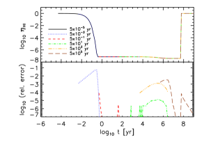
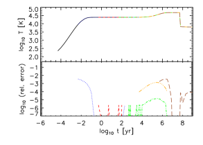
Figure 2: Test 1. Single gas parcel with prescribed photoionisation rate. The top panels show the evolution of the neutral hydrogen fraction (left) and temperature (right) for simulations with different time steps $\Delta t$ (in the range $5\times 10^{-5}~{}\mbox{yr}-5\times 10^{5}~{}\mbox{yr}$), as indicated in the legend in the top left panel. All simulations start at time $t=0$ and evolve the gas parcel on subcycle steps $\delta t=\min(f\tau_{\rm eq},\Delta t)$, where $\tau_{\rm eq}$ is the time scale on which the gas parcel approaches equilibrium and $f=0.01$ is a dimensionless parameter that controls the accuracy of the subcycling. Note that the first output occurs only at the end of the first time step, i.e., at time $t=\Delta t$, which is different for the different simulations. The bottom panels show the relative errors of the evolution shown in the top panels with respect to the evolution obtained from the simulations with the next smaller time step. The relative errors are small, $\lesssim 1\%$, except during a brief phase of rapid evolution in the ionised fraction. The relative error can be reduced by choosing a smaller value for the accuracy parameter $f$.

Here we test the subcycling approach to the computation of the coupled evolution of the non-equilibrium ionisation balance and temperature of gas exposed to ionising radiation that we have introduced in Sec. 4.2. Our aim is to demonstrate that, given a flux impinging on a gas parcel (or, equivalently, a photoionisation rate experienced by this parcel), the subcycling allows for an accurate computation of the evolution of its ionisation state and temperature, independent of the size of the RT time step $\Delta t_{\rm r}$.

The setup of the test is as follows. We simulate the evolution of the ionisation state of an optically thin gas parcel with hydrogen number density $n_{\rm H}=1~{}~{}\mbox{cm}^{-3}$. For simplicity and clarity of the presentation, we set the hydrogen mass fraction to $X=1$ (i.e., no helium). The simulation starts at time $t=0$ with a fully neutral parcel with initial temperature $T=10^{2}~{}\mbox{K}$. We then apply a photoionising flux of $F=10^{12}~{}~{}\mbox{s}^{-1}~{}\mbox{cm}^{-2}$ with a blackbody spectrum of characteristic temperature $T_{\rm bb}=10^{5}~{}\mbox{K}$. Consequently, the parcel becomes highly ionised and is heated to a temperature $T\sim 10^{4}~{}\mbox{K}$. After $t=50~{}\mbox{Myr}$ we switch off the ionising flux and the parcel recombines and cools. The simulation ends at $t_{\rm end}=1~{}\mbox{Gyr}$. The test here is identical to Test 0 presented in Iliev et al. (2006a), except for the switch-off time (Iliev et al., 2006a used $t_{\rm end}=0.5~{}\mbox{Myr}$).

We employ a grey photoionisation cross-section $\langle{\sigma}_{\gamma\rm HI}\rangle=1.63\times 10^{-18}~{}\mbox{cm}^{2}$ (Sec. 3.1), yielding a photoionisation rate $\Gamma_{\gamma\rm HI}=1.63\times 10^{-6}~{}\mbox{s}^{-1}$. We assume that each photoionisation adds $\langle\epsilon_{\rm HI}\rangle=6.32~{}\mbox{eV}$ to the internal energy of the gas (Sec. 3.2), which corresponds to the optically thin limit. We solve the equations for the evolution of the ionisation state and temperature of the gas parcel by subcycling them on subcycle time steps $\delta t$ over consecutive time intervals $\Delta t$. Note that in a full RT computation these intervals would correspond to the RT time steps $\Delta t_{\rm r}$. Here we distinguish between $\Delta t$ and $\Delta t_{\rm r}$ only because in this test we are considering a single gas parcel with prescribed photoionisation rate and do not perform RT simulations. The dimensionless parameter $f$ that controls the size of the subcycling steps $\delta t$ (and hence the accuracy of the subcycling) is set to $f=10^{-2}$. When computing Compton cooling rates off the cosmic microwave background, we assume a redshift $z=0$.

Fig. 2 shows the results. The top left and top right panels show the evolution of the neutral hydrogen fraction and the temperature, respectively, for simulations with time steps $\Delta t=5\times(10^{-5}$, $10^{-3}$, $10^{-1}$, $10^{1}$, $10^{3}$, $10^{5})~{}\mbox{yr}$. Note that in order to limit the computation time, not all of the simulations have been evolved until the end of the simulation time. They were stopped once their simulation time overlapped with that of the simulation with the next larger time step. The earliest output of a given simulation is at $t=\Delta t$ (and hence, in Fig. 2, different curves start at different times), but all simulations started at $t=0$ and were numerically evolved on subcycle time steps $\delta t<\Delta t$ as described in Sec. 4.2.

The gas parcel quickly approaches photoionisation equilibrium, reaching its equilibrium neutral fraction after $\sim 10$ (photo-)ionisation time scales ($\tau_{\rm ion}\equiv\Gamma_{\gamma\rm HI}^{-1}\approx 0.02~{}\mbox{yr}$). During this period, photoheating raises its temperature to $T\approx 2\times 10^{4}~{}\mbox{K}$. Around $t\sim 10^{5}~{}\mbox{yr}$, the neutral fraction exhibits a slight decrease. As noted in Iliev et al. (2006a), this behaviour is caused by the decrease in the recombination rate due to the rise in temperature that can be observed at this time. The fact that the temperature still evolves after the neutral fraction reached its equilibrium value means that thermal equilibrium is reached on a larger time scale than photoionisation equilibrium. Note that the thermal equilibrium phase is missed in the test simulations of Iliev et al. (2006a) because these simulations were stopped at a much earlier time.

The observed behaviour can be understood as follows. When thermal equilibrium is approached from a temperature lower than the equilibrium temperature, the net cooling rate is approximately given by the photoheating rate. In photoionisation equilibrium, the photoheating rate is proportional to the recombination rate. The time scale $\tau_{\rm u}\equiv u/(du/dt)$ to reach thermal equilibrium can therefore be expressed in terms of the recombination time $\tau_{\rm rec}\equiv 1/(n_{\rm e}\alpha_{\rm HII})$,

$$\tau_{\rm u} = \frac{(3/2)nk_{\rm B}T}{n_{\rm H}^{2}h_{\gamma}}$$ (27)

$$= \frac{(3/2)nk_{\rm B}T}{n_{\rm HII}n_{\rm e}\alpha_{\rm HII}\langle\epsilon_{\rm HI}\rangle}$$ (28)

$$= \frac{(3/2)nk_{\rm B}T}{\langle\epsilon_{\rm HI}\rangle n_{\rm HII}}\tau_{\rm rec}$$ (29)

$$\sim \tau_{\rm rec},$$ (30)

where in the last step we assumed that the gas is highly ionised, i.e. $n_{\rm HII}\approx n_{\rm H}\approx n/2$, and that $T\approx 10^{4}~{}\mbox{K}$. The recombination time (and hence the cooling time) is much larger than the time $\tau_{\rm eq}\equiv(\tau_{\rm ion}\tau_{\rm rec})/(\tau_{\rm ion}+\tau_{\rm rec})$ to reach ionisation equilibrium which asymptotes to $\tau_{\rm ion}$ for $\tau_{\rm ion}\ll\tau_{\rm rec}$ (see also the discussion in Sec. 5.1 in Paper I). Here, $\tau_{\rm ion}=\Gamma_{\gamma\rm HI}^{-1}\approx 0.02~{}\mbox{yr}$ and $\tau_{\rm rec}\approx 10^{5}~{}\mbox{yr}$. Accordingly, thermal equilibrium is reached much later than photoionisation equilibrium.

After thermal equilibrium has been reached, the ionising flux is switched off and the parcel recombines and cools. Once it has cooled to a temperature $T\lesssim 10^{4}~{}\mbox{K}$, cooling becomes inefficient. The temperature of the recombining parcel therefore remains roughly constant.

In the bottom panels of Fig. 2 we quantify the accuracy of our subcycling approach. Ideally, we would like to compare the numerical results to an exact analytical reference solution. However, such a solution exists only for the case of a constant temperature (see, e.g., the appendix in Dove & Shull, 1994). Instead, we therefore show the relative error of the evolutions shown in the top panel with respect to the evolutions obtained from the simulation with the next smaller time step.

For all our choices of the time step $\Delta t$ and for most of the simulation time the relative errors are small, $\lesssim 1\%$ or even much smaller. During the initial phase of rapid evolution the relative error in the ionised fraction briefly becomes as large as $10\%$. In practice, such errors will have little impact on the results of RT simulations if photons are conserved and if the equilibrium solution is still obtained with high accuracy (as is the case). Moreover, relative differences of order $10\%$ are already implied by uncertainties in current atomic data used to compute the ionisation and recombination rates and the radiative heating and cooling rates (as will be discussed in Sec. 5.2.2). Note that the relative error can be reduced by lowering the numerical factor $f$, which controls the size of the subcycle steps and hence the integration accuracy. We conclude that the results of the subcycling are insensitive to the size of the simulation time step.

In summary, we have demonstrated that our subcycling recipe accurately computes, independently of the size of the RT time step, the combined evolution of the neutral fraction and temperature of gas exposed to hydrogen-ionising radiation. In the following sections we will employ the subcycling to compute the species fractions and temperature of gas particles in RT simulations.

5.2 HII region expansion. Reference results and comparisons of multi-frequency and grey solutions

In the next section (Sec. 5.3) we will apply our new implementation of traphic to compute the evolution of the ionisation state and temperature around an ionising source surrounded by gas of constant density. This is an idealised test problem designed to facilitate the verification of our implementation through the direct comparison to results obtained with an improved version of our one-dimensional (1-d) RT code (Pawlik & Schaye, 2008; hereafter referred to as tt1d, which stands for TestTraphic1D), which solves the rate equations using the same techniques (and code) as traphic, as well as to published reference results obtained with other RT codes for the same test problem (Iliev et al., 2006a). In this section we present these reference results. We also discuss the applicability of the grey approximation for solving multi-frequency RT problems.

We start in Sec. 5.2.1 by presenting reference solutions obtained with our 1-d RT code tt1d for the case of hydrogen-only gas at fixed temperature. This is an important case because it allows analytical solutions to be derived against which the numerical results obtained with tt1d can be compared. Then, in Sec. 5.2.2, we compare the performance of tt1d in a simulation of hydrogen-only gas in which the gas temperature is allowed to evolve due to photoheating and radiative cooling to published numerical results obtained for the same problem. Finally, in Sec. 5.2.3, we discuss results from simulations with tt1d in which the gas also contains helium.

5.2.1 HII region in pure hydrogen gas at fixed temperature

In this section we discuss the RT problem of an expanding HII region. Despite its simplicity, an analytical solution to this problem cannot generally be obtained, even if the gas densities are assumed to be non-evolving (as is the case throughout this work). This is because the coupling between the ionisation and temperature state through the dependence of the collisional ionisation, recombination and cooling rates on the temperature and species fractions impedes the evaluation of the governing differential equations (Eqs. 1 - 6 and 12).

To provide an approximate point of reference, we recall the evolution of an HII region at fixed gas temperature, for which an analytical solution is known (under the approximation that the ionised region is fully ionised; we will also ignore collisional ionisations, although this is not necessary). We have reviewed this solution in Paper I, where we showed that the radius of the ionised sphere around a source of ionising luminosity $\dot{\mathcal{N}}_{\gamma}$ that is located in a homogeneous hydrogen-only medium of density $n_{\rm H}$ is given by

$$r_{\rm I}(t)=r_{\rm s}(1-e^{-t/\tau_{\rm s}})^{1/3},$$ (31)

where $r_{\rm s}=[3\dot{\mathcal{N}}_{\gamma}/(\alpha_{\rm BHII}n_{\rm H}^{2})]^{1/3}$ is the Strömgren radius and $\tau_{\rm s}=1/(\alpha_{\rm BHII}n_{\rm H})$ is the Strömgren time scale, which equals the recombination time for fully ionised gas. In some of our comparisons we will employ this approximate point of reference. We will refer to it as an analytical approximation. On the other hand, because of the lack of an accurate analytical solution, we will mostly employ results obtained with our 1-d RT code tt1d in our benchmarking below. For this reason, we will first discuss its performance.

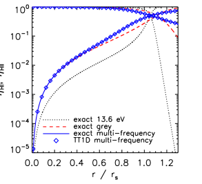
Figure 3: Photoionisation equilibrium profiles of the neutral and ionised fraction around a single blackbody source in a homogeneous hydrogen-only medium. The numerical result obtained with tt1d (diamonds) shows excellent agreement with the analytically computed exact results (Eq. 32; blue solid curve). For comparison, we also show the analytically computed exact solutions assuming the grey approximation (red dashed curve) and the monochromatic treatment used in Test 1 of Paper I (black dotted curve). The grey approximation agrees with the exact solution in the optically thin limit (i.e., in the absence of spectral hardening), while the monochromatic treatment fails at all distances because it implies photoionisation rates inconsistent with the spectrum of the considered blackbody source.

We start by verifying our multi-frequency treatment in tt1d by comparing its performance in a simple HII region test problem to the corresponding equilibrium solution that can be derived analytically (except for a numerical evaluation of the integrals involved). The test consists of simulating the spherically symmetric growth of the ionised region around a single ionising source in a homogeneous hydrogen-only medium at fixed temperature. The source has a blackbody spectrum with temperature $10^{5}~{}\mbox{K}$ and emits radiation with an ionising luminosity $\dot{\mathcal{N}}_{\gamma}=5\times 10^{48}~{}\mbox{photons}~{}\mbox{s}^{-1}$. The gas density is $n_{\rm H}=10^{-3}~{}\mbox{cm}^{-3}$. The initial ionised fraction is assumed to be $\eta_{\rm HII}=0$, and we use a recombination coefficient $\alpha_{\rm BHII}=2.59\times 10^{-13}~{}\mbox{cm}^{3}~{}\mbox{s}^{-1}$, independent of radius and time. Collisional ionisation is not included. For reference, with the physical parameters mentioned above, the Strömgren time is $\tau_{\rm S}=122.4~{}\mbox{Myr}$ and the Strömgren radius is $r_{\rm S}=5.4~{}\mbox{kpc}$. The spatial resolution, the time step and the number of frequency bins used in the simulation with tt1d are chosen such as to achieve numerical convergence.

In Fig. 3 we show the neutral (ionised) fraction profile in photoionisation equilibrium. Diamonds show the result of the simulation with tt1d (at $t=2000~{}\mbox{Myr}$). The blue solid curve indicates the exact equilibrium solution obtained by solving (e.g., Osterbrock, 1989)

$$\frac{\eta_{\rm HI,eq}(r)n_{\rm H}}{4\pi r^{2}}\int d\nu\ \dot{\mathcal{N}}_{\gamma}(\nu)e^{-\tau_{\nu}}\sigma_{\nu}=\eta_{\rm HII,eq}^{2}(r)n_{\rm H}^{2}\alpha_{\rm BHII},$$ (32)

where the frequency-dependent optical depth $\tau_{\nu}(r)$ is given by

$$\tau_{\nu}(r)=n_{\rm H}\sigma_{\nu}\int_{0}^{r}dr^{\prime}\ \eta_{\rm HI,eq}(r^{\prime}).$$ (33)

The simulation result is in excellent agreement with the exact equilibrium solution, verifying our multi-frequency implementation of tt1d. For comparison, we also show the exact equilibrium solution assuming that the radiation is monochromatic (dotted black curve) with a photoionisation cross-section evaluated at the ionisation threshold, i.e. $\sigma_{\gamma\rm HI}=6.3\times 10^{-18}~{}\mbox{cm}^{2}$. We also show the exact equilibrium solutions in the grey treatment, i.e. using the average cross-section $\langle\sigma_{\gamma\rm HI}\rangle=1.63\times 10^{-18}~{}\mbox{cm}^{2}$ (dashed red curve).

The reason for the differences between the results of the multi-frequency computation and the results of the grey and monochromatic computation can be readily understood. The absorption cross-section for ionising photons is a strongly decreasing function of the photon energy. The ionising photons with the lowest energy are therefore preferentially absorbed, which leads to an increase in the typical photon energy with distance. This effect is referred to as spectral hardening. Because the photon mean free path is inversely proportional to the absorption cross-section, spectral hardening increases the width of the ionisation front with respect to that obtained in the absence of spectral hardening. Note that spectral hardening only becomes important for large optical depths, which explains why the grey approximation reproduces the multi-frequency solution at small distances where the optical depth is low. The monochromatic approximation, on the other hand, implies an inappropriate value for the photoionisation rate and hence fails to describe the present multi-frequency problem at all distances from the source. Note that both the grey and the monochromatic approximation will provide a better description of the multi-frequency problem for sources with a softer radiation spectrum.

5.2.2 HII region in pure hydrogen gas with an evolving temperature

Having demonstrated the validity of our multi-frequency treatment with tt1d, we now repeat the test problem from the previous section but this time we account for the self-consistent evolution of the gas temperature due to photoheating and radiative cooling. The physical parameters for the test are taken from Iliev et al. (2006a). We consider an ionising source embedded in a homogeneous hydrogen-only density field with number density $n_{\rm H}=10^{-3}~{}\mbox{cm}^{-3}$. The source emits $\dot{\mathcal{N}}_{\gamma}\equiv\int d\nu\ \dot{\mathcal{N}}_{\gamma}(\nu)=5\times 10^{48}~{}\mbox{ionising photons}~{}\mbox{s}^{-1}$ with a blackbody spectral shape $\dot{\mathcal{N}}_{\gamma}(\nu)$ corresponding to a blackbody temperature $T_{\rm bb}=10^{5}~{}\mbox{K}$. The test described here is identical to Test 1 in Paper I, except that now the gas temperature is allowed to vary due to heating and cooling processes as described in Sec. 3.2 (with Compton cooling off the redshift $z=0$ cosmic microwave background included) and that collisional ionisation is included. The gas is assumed to have an initial ionised fraction $\eta_{\rm HII}=1.2\times 10^{-3}$ (approximately corresponding to the ionised fraction implied by collisional ionisation equilibrium at the temperature $T=10^{4}~{}\mbox{K}$). Its initial temperature is set to $10^{2}~{}\mbox{K}$. As before, the spatial resolution, the time step and the number of frequency bins used in the simulation with tt1d are chosen such as to achieve numerical convergence.

Fig. 4 shows the neutral (ionised) fraction and temperature profiles at time $t=100~{}\mbox{Myr}$ using tt1d (black solid curves). We compare these multi-frequency results to results obtained using the grey approximation, i.e. using an average cross-section $\langle\sigma_{\gamma\rm HI}\rangle=1.63\times 10^{-18}~{}\mbox{cm}^{2}$ and grey photoheating rates. We employ grey photoheating rates computed in the optically thin limit (red dotted curves), according to which each photoionisation adds $\langle\epsilon_{\rm HI}\rangle=6.32~{}\mbox{eV}$ to the internal energy of the gas, and in the optically thick limit (blue dashed curves), in which case each photoionisation adds $\langle\epsilon^{\rm thick}_{\rm HI}\rangle=16.01~{}\mbox{eV}$ to the internal energy of the gas (Sec. 3.2). We employ the labels grey thin and grey thick to distinguish the two grey simulations from each other. We also show the results obtained (in three-dimensional RT simulations) with the RT codes c²-ray (Mellema et al., 2006), crash (Ciardi et al., 2001; Maselli, Ferrara, & Ciardi, 2003) and ftte (Razoumov & Cardall, 2005) for the same test problem, as published in Iliev et al. (2006a).

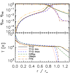
Figure 4: Test 2 (using tt1d). Comparison of the grey approximations with the full multi-frequency solution. The figure shows spherically averaged profiles of neutral (ionised) fraction (top) and temperature (bottom) at time $t=100~{}\mbox{Myr}$. The black solid curve shows the multi-frequency solution. The red dotted (blue dashed) curve shows its grey approximation assuming photoheating rates computed in the optically thin (thick) limit. The grey and multi-frequency simulations show clear differences close to and beyond the ionisation front, where the large optical depth causes spectral hardening of the emitted blackbody spectrum. For reference, we also show results obtained with other RT codes as published in Iliev et al. (2006a). The green dash-dotted and black solid curves in the top panel are difficult to distinguish because they fall nearly on top of each other. The differences between these results at large distances mainly reflect the differences in the numerical treatment of multi-frequency radiation in these codes. Most of the differences close to the ionising source have their origin in the use of different assumptions for computing photoheating rates, as the comparison to the results obtained with tt1d reveals.

The differences in the neutral fractions between the grey and the multi-frequency simulations that we have discussed above for Fig. 3 are again clearly visible (top panel of Fig. 4). The grey thin simulation yields results that asymptote to those obtained in the multi-frequency simulation at small distances from the ionising source. At large distances, i.e. near the ionisation front and beyond, on the other hand, the multi-frequency simulation implies significantly larger ionised fractions than those implied by this grey simulation. This is because the photon mean free path is larger in the multi-frequency simulation than in the grey simulations due to spectral hardening, leading to a smoother transition of the neutral fraction between the highly ionised gas interior to and the neutral gas far ahead of the ionisation front.

The grey thick simulation yields neutral fractions that are very similar to those found in the grey thin simulation. However, the grey thick simulation yields slightly lower neutral fractions than the grey thin simulation, since it yields slightly larger temperatures, and thus smaller recombination rates, throughout the ionised region (bottom panel of Fig. 4). In contrast to the grey thin simulation, the neutral fractions obtained in the grey thick simulation therefore do not asymptote to those obtained in the multi-frequency simulation at small distances to the ionising source. Instead, they remain systematically too small.

The differences between the grey and multi-frequency simulations (and between the grey thin and grey thick simulations) become particularly apparent when inspecting the corresponding temperature profiles. The multi-frequency simulation yields substantially higher gas temperatures ahead of the ionisation front. This pre-heating is a simple consequence of the increase in the photon mean free path above that in the grey simulations. As already noted, at fixed radii the grey thick simulation shows systematically higher gas temperatures than the grey thin simulation. The reason is that in the optically thin limit the contribution of high-energy photons to the photoheating rate is reduced due to the weighting by the absorption cross-section $\sigma_{\rm HI}(\nu)$, which is a strongly decreasing function of the photon energy. Observe that the temperatures (like the neutral fractions) obtained in the grey thin simulation asymptote to those obtained in the multi-frequency simulation at small distances to the ionising source, while the temperatures in the grey thick simulation are too high.

We summarise our discussion of the differences between the grey and multi-frequency simulations for the present problem by noting that the use of the grey approximation leads to neutral fractions and temperatures that generally are very different from those obtained in detailed multi-frequency simulations. At large optical depths, the neutral fractions are systematically too high and the temperatures too low due to the lack of spectral hardening. The grey treatment yields neutral fractions and temperatures that asymptote to those obtained in the corresponding multi-frequency simulation at small distances to the ionising source when photoheating rates are computed in the optically thin limit, i.e. using Eq. 16. When computing photoheating rates in the optically thick limit, i.e. using Eq. 17, the neutral fractions and temperatures do not asymptote to the correct values at small distances to the ionising source, i.e. the values in the multi-frequency simulation. Consequently, when one invokes the grey approximation to compute the thermal structure of ionised regions, one should compute photoheating rates in the optically thin limit. Photoheating rates in the optically thick limit should only be employed when considering the thermal balance of an ionised region as a whole. Ideally, one would perform detailed multi-frequency simulations and simply dispense with the grey approximation.

We now discuss the results of our simulations with tt1d with respect to those obtained with c²-ray, crash and ftte for the same test problem (Iliev et al., 2006a). We note that the simulation with crash employed multiple frequency bins, while the one with ftte was done using a single frequency bin and computing photoionisation and optically thick photoheating in the grey approximation (Alexei Razoumov, private communication). Finally, c²-ray used a hybrid method (Garrelt Mellema, private communication): the absorption of ionising radiation was computed as a function of frequency, but each photoionisation injected the same amount of energy, regardless of the frequency of the absorbed photon. This method thus accounts fully for the spectral hardening of the radiation but ignores it when computing photoheating rates.

There are noticeable differences in the results obtained with these three codes. At large distances from the ionising source, i.e. close to and beyond the ionisation front, most of these differences may be attributed to differences in the multi-frequency implementation, leading to differences in the spectral hardening of the emitted blackbody spectrum. At these distances, the neutral fractions obtained in our grey simulations agree closely with those obtained with ftte, while the neutral fractions obtained in our multi-frequency simulations closely agree with (and are, in fact, nearly identical to) those obtained with c²-ray, as expected from our discussion above. We note that the fact that the neutral fractions obtained with crash are systematically too large may indicate that the radiation field was too poorly sampled (see Maselli, Ferrara, & Ciardi, 2003, in particular their Fig. 2, for a thorough discussion).

The results, however, show also significant differences in the neutral fractions and temperatures close to the ionising source, where the gas is close to optically thin and the emitted blackbody radiation spectrum is not severely deformed due to spectral hardening. Some of these differences can be attributed to the fact that the different codes employ different expressions for cross-sections, recombination and cooling rates. As demonstrated in Iliev et al. (2006a) (their Fig. 4), different recombination and cooling rates may only account for differences in the neutral fraction and temperature of at most $\lesssim 10\%$. We have verified this by employing the rates used with the different codes (Table 2 in Iliev et al., 2006a) in simulations with tt1d.

Most of the differences close to the ionising source may instead be traced back to the use of different assumptions underlying the computation of the photoheating rates. In fact, the temperatures obtained with crash are in very good agreement with the temperatures obtained in our multi-frequency and grey thin simulations, while the temperatures obtained by ftte and c²-ray are in excellent agreement with the temperatures in our grey thick simulation.

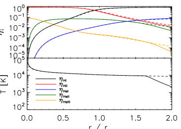
Figure 5: Comparison of the results from a simulation with tt1d (solid curves) with those from a simulation with cloudy (dashed curves) for the HII region test problem described in Sec. 5.3 (assuming $X=0.75$, $Y=1-X$). Note that the results computed with cloudy correspond to equilibrium ($t\to\infty$), while the results computed with tt1d correspond to a time $t=2000~{}\mbox{Myr}$ (which is much larger than the recombination time on which the gas reaches thermal and ionisation equilibrium). The results obtained with tt1d are nearly indistinguishable from those obtained with cloudy for all radii at which equilibrium has been reached.

5.2.3 HII region in gas containing hydrogen and helium with an evolving temperature

Finally, we test the ability of tt1d to accurately compute the ionisation and temperature structure in gas containing both hydrogen and helium by comparing results obtained with tt1d with results obtained with the photoionisation code cloudy (version 08.00; last described by Ferland et al., 1998) for the same test problem. Note that cloudy assumes ionisation equilibrium.

As before we consider an ionising source with blackbody spectrum of temperature $T=10^{5}~{}\mbox{K}$ with an ionising luminosity of $5\times 10^{48}~{}\mbox{s}^{-1}$ in gas of density $n_{\rm H}=10^{-3}$, but we now assume $X=0.75$ and $Y=1-X$. cloudy includes considerably more physics than tt1d. To facilitate a direct comparison, we therefore keep the setup of the simulations as simple as possible: we assume that there is no radiative coupling between hydrogen and helium, i.e., photons emitted due to recombination of helium do not lead to ionisations of hydrogen, and compute recombinations in the Case A (Sec. 3.1.2) limit.

Fig. 5 shows the ionised fractions and temperatures computed with tt1d at time $t=2000~{}\mbox{Myr}$. It also shows the results obtained with cloudy, which correspond to a time $t\to\infty$. The agreement between tt1d and cloudy is excellent. The results only differ at radii where (in the simulation with tt1d) equilibrium has not yet been reached. Thus, tt1d yields equilibrium ionisation and temperature profiles that are almost indistinguishable from those obtained with a well-tested and widely employed state-of-the-art photoionisation code.

5.3 Test 2: HII region expansion. TRAPHIC

In this section we apply our new implementation of traphic to compute the evolution of the ionisation state and temperature around an ionising source surrounded by gas of constant density. This idealised test problem captures the main characteristics of a thermally coupled RT simulation that we wish to verify: conservation of the number of ionising photons, which ensures that the final ionised region attains the correct size, and conservation of the associated energy, which, together with an accurate implementation of the relevant cooling processes, ensures that the ionised region settles into the correct thermal structure. The physical parameters for the test are identical to those employed to obtain the reference solutions presented in Sec. 5.2.2 but, for definiteness, we repeat the problem description here.

We consider an ionising source embedded in a homogeneous hydrogen-only density field with number density $n_{\rm H}=10^{-3}~{}\mbox{cm}^{-3}$. The source emits $\dot{\mathcal{N}}_{\gamma}\equiv\int d\nu\ \dot{\mathcal{N}}_{\gamma}(\nu)=5\times 10^{48}~{}\mbox{ionising photons}~{}\mbox{s}^{-1}$ with a blackbody spectral shape $\dot{\mathcal{N}}_{\gamma}(\nu)$ corresponding to a blackbody temperature $T_{\rm bb}=10^{5}~{}\mbox{K}$. The test described here is identical to Test 1 in Paper I, except that now the gas temperature is allowed to vary due to heating and cooling processes as described in Sec. 3.2 (with Compton cooling off the redshift $z=0$ cosmic microwave background included) and that collisional ionisation is included. The gas is assumed to have an initial hydrogen ionised fraction $\eta_{\rm HII}=1.2\times 10^{-3}$ (approximately corresponding to the ionised fraction implied by collisional ionisation equilibrium at the temperature $T=10^{4}~{}\mbox{K}$). Its initial temperature is set to $10^{2}~{}\mbox{K}$.

First, in Sec. 5.3.1, we consider the case in which radiation is transported using a single frequency bin in the grey optically thin approximation in pure hydrogen gas. We employ the grey approximation to allow for a more direct comparison with the results presented in Paper I. In Sec. 5.3.2 we will also briefly discuss the performance of traphic in multi-frequency simulations in gas containing both hydrogen and helium.

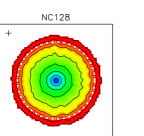
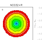
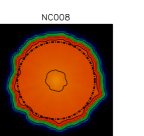
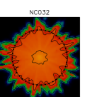
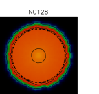
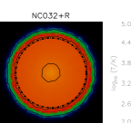
Figure 6: Test 2 (using traphic). Neutral fraction (top row) and temperature (bottom row) at time $t=100~{}\mbox{Myr}$ in a slice through the centre of the simulation box. From left to right: angular resolution $N_{\rm c}=8,32$, $128$ (all without resampling) and $32$ (with resampling of the particle positions after every 10th RT time step, as indicated by the letter ‘R’ in the panel titles). The dot-dashed circles indicate the position of the ionisation front, calculated using the analytical approximation (Eq. 31). Contours show neutral fractions of $\eta_{\rm HI}=0.9,0.5$, $\log_{10}\eta_{\rm HI}=-1,-1.5,-2,-2.5,-3,-3.5$ and temperatures $\log_{10}(T/{\rm K})=(3,4,4.2)$ (from the outside in). The crosses in the top row indicate the spatial resolution $\langle 2\tilde{h}\rangle$.

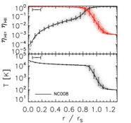
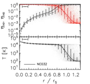
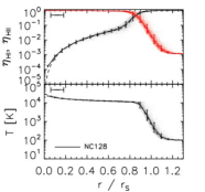
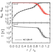
Figure 7: Test 2 (using traphic). Scatter plots and profiles of the neutral (ionised) fraction and temperature at time $t=100~{}\mbox{Myr}$ for simulations with angular resolution $N_{\rm c}=8$ (left), $32$ (middle) and $128$ (right). Top row: No resampling. Bottom row: Resampling of the particle positions after every 10th RT time step (indicated by the letter ‘R’ in the legends). Each dot represents the neutral fraction (ionised fraction, temperature) of a single SPH particle (only a randomly chosen subset of $10\%$ of all particles is shown). Solid curves show the median neutral fraction (ionised fraction, temperature) in spherical bins around the ionising source. The vertical error bars enclose $68.3\%$ of the particles in each bin. Dashed curves indicate the reference solution obtained with our 1-d RT code tt1d. The horizontal error bars in the upper left corners indicate the spatial resolution. The results of all simulations are in excellent agreement with the reference solution. Without the resampling, the results are noisier if $N_{\rm c}\approx\tilde{N}_{\rm ngb}$ (top middle panel).

5.3.1 HII region expansion: grey thin, hydrogen-only

The numerical realisation of the initial conditions is similar to that used for Test 1 in Paper I. The ionising source is located at the centre of a simulation box with side length $L_{\rm box}=13.2~{}\mbox{kpc}$. The box boundaries are photon-transmissive, i.e., photons leaving the box are lost from the computational domain. We assign each SPH particle a mass $m=n_{\rm H}m_{\rm H}L_{\rm box}^{3}/N_{\rm SPH}$, where $N_{\rm SPH}$ is the total number of SPH particles. The positions of the SPH particles are chosen to be glass-like (e.g., White, 1996). Glass-like initial conditions imply a more regular distribution of particles in space when compared to that obtained from a Monte Carlo sampling of the density field. The SPH smoothing kernel is computed and the SPH densities are found using the SPH formalism implemented in gadget-2, with $N_{\rm ngb}=48$.

Photons are transported using a single frequency bin assuming the grey approximation in the optically thin limit. We therefore employ a photoionisation cross-section $\langle\sigma_{\gamma\rm HI}\rangle=1.63\times 10^{-18}~{}\mbox{cm}^{2}$ (Sec. 3.1) and assume that each photoionisation adds $\langle\epsilon_{\rm HI}\rangle=6.32~{}\mbox{eV}$ to the thermal energy of the gas (Sec. 3.2). The RT time step is set to $\Delta t_{\rm r}=10^{-2}~{}\mbox{Myr}$ to facilitate a comparison to Test 1 in Paper I. For the same reason, we limit ourselves to solving the time-independent RT equation and propagate photons during each time step only from a given particle to its direct neighbours. All simulations presented in this section employ $N_{\rm SPH}=64^{3}$ SPH particles, which are evolved for a total of $500~{}\mbox{Myr}$. Some of our simulations employ the resampling technique introduced in Paper I to reduce artifacts due to the particular setup of the initial conditions. Briefly, each SPH particle is, within its spatial resolution element whose size is determined by the diameter of the SPH kernel, $2h$, from time to time offset randomly from its initial position. For comparison, we repeat all simulations without employing this technique. We perform simulations with different angular resolutions. Figs. 6 and 7 show our results.

In Fig. 6 we present slices through the centre of the simulation box showing the neutral fraction (top row) and temperature (bottom row) at time $t=100~{}\mbox{Myr}$. In each row, the three left-most panels show results from simulations with angular resolution $N_{\rm c}=8,32$ and $128$ and no resampling of the particle positions applied and the right-most panel shows results from a simulation with angular resolution $N_{\rm c}=32$ and resampling of the particle positions every 10th RT time step. In each panel we indicate, as a point of reference, the analytical approximation for the position of the ionisation front (Eq. 31) by a dash-dotted circle.

Interior to the ionisation front the gas is highly ionised and photo-heated to typical temperatures $T\approx 1.5\times 10^{4}~{}\mbox{K}$ (with maximum temperatures $T\approx 2\times 10^{4}~{}\mbox{K}$). The runs that did not employ the resampling show slight deviations from the expected spherical shape which depend on the angular resolution. As discussed in Paper I, the deviations are caused by the particular arrangement of the SPH particles. Reducing this particle noise, which is strongest when $N_{\rm c}\approx\tilde{N}_{\rm ngb}$, was the motivation for introducing the resampling technique. Indeed, the distribution of neutral fractions and temperatures from the simulation that employed the resampling of the density field is spherically symmetric to a high degree.

In Fig. 7 we compare the median profiles of the neutral fraction (left-hand panel) and the temperature (right-hand panel) at time $t=100~{}\mbox{Myr}$ obtained from the three-dimensional simulations with traphic (solid curves with error bars) to the reference simulation obtained with our 1-d RT code tt1d (dashed curves). The results of all simulations are in excellent agreement with the reference result. The small deviations that are present very close to the ionising source and in regions where the profile gradients are steep are due to the finite spatial resolution (indicated with horizontal error bars in the top left corners of the panels). The effect of resampling in reducing noise can most clearly be seen when comparing the simulations with angular resolution $N_{\rm c}=\tilde{N}_{\rm ngb}=32$ with each other (middle panels). Note that for the simulation with the highest angular resolution that we have considered here ($N_{\rm c}=128$), the resampling slightly reduces the agreement with the reference simulation because it introduces additional scatter. This scatter is consistent with the spatial resolution employed.

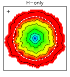
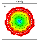
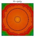
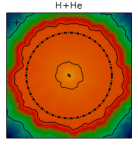
Figure 8: Test 2 (using traphic). Multi-frequency transport and effects of the inclusion of helium (Sec. 5.3.2). Neutral hydrogen fraction $\eta_{\rm HI}$ (top panels) and temperature (bottom panels) at time $t=100~{}\mbox{Myr}$ in a slice through the centre of the simulation box. The left and right panels show, respectively, results from simulations of an ionising source in gas of pure hydrogen ($X=1$) and gas with primordial abundances ($X=0.75$, $Y=1-X$). Except for this difference in the helium abundance, both simulations are identical; in particular, they both make use of five frequency bins to transport the emitted $10^{5}~{}\mbox{K}$ blackbody photons. The panels can be compared with the left-most panels of Fig. 6, which show results from a simulation that is identical except that it used a single frequency bin and the grey optically thin approximation. As in Fig. 6, the dot-dashed circle indicates the position of the ionisation front, calculated using the analytical approximation (Eq. 31). Contours show neutral fractions of $\eta_{\rm HI}=0.9,0.5$ , $\log_{10}\eta_{\rm HI}=-1,-1.5,-2,-2.5,-3,-3.5$ and temperatures $\log_{10}(T/\rm{K})=(3,4,4.2,4.4)$ (from the outside in). The colour coding is the same as in Fig. 6. The crosses indicate the spatial resolution $\langle 2\tilde{h}\rangle$.

5.3.2 HII region expansion: multi-frequency, hydrogen and helium

Next we demonstrate the ability of traphic to accurately solve the present multi-frequency problem in gas of primordial composition (i.e., in the presence of helium) and using multiple frequency bins. For brevity, we discuss only a single simulation with particle number $N=64^{3}$ and angular resolution $N_{\rm c}=8$. We have verified that simulations with other choices for these parameters show the expected behaviour.

We perform two simulations. The first simulation assumes a hydrogen mass fraction $X=1$. The second simulation assumes a hydrogen mass fraction $X=0.75$ and a helium mass fraction $Y=1-X$. We set the initial ionised helium fractions to zero, $\eta_{\rm HeII}=\eta_{\rm HeIII}=0$. All other physical parameters are as in the previous section. For both simulations we use the same number of frequency bins, $N_{\nu}=5$ (starting at $13.6~{}\mbox{eV}$, $24.6~{}\mbox{eV}$, $35.5~{}\mbox{eV}$, $54.4~{}\mbox{eV}$ and $75.0~{}\mbox{eV}$, with the last bin extending to infinity). The photoionisation cross-section and excess energy associated with each bin are obtained from averaging over a blackbody spectrum of temperature $10^{5}~{}\mbox{K}$, assuming the optically thin limit (Eqs. 9 and 16).

The motivation behind our choice to use a small number of frequency bins is that in realistic simulations that will be computationally more expensive, limited resources will require the usage of as few frequency bins as possible. Our results below show that a number as low as five (and perhaps even as low as three, see Sec. 5.4) may be sufficient to capture the main effects associated with multi-frequency radiation transport.

Fig. 8 shows the neutral hydrogen fractions (top) and temperatures (bottom) in a slice through the centre of the simulation box for the simulation without (left) and with (right) helium. The panels can be compared with the left-most panels of Fig. 6, which show results from an identical simulation except that it used a single frequency bin and the grey, optically thin approximation. The effect of spectral hardening is most visible in the panels showing the temperature, with the multi-frequency simulations showing a substantial pre-heating ahead of the ionisation front. Interestingly, the simulation that includes helium shows slightly less pre-heating (and pre-ionisation) than the one that assumes pure hydrogen.

The solid curves in Fig. 9 show median profiles of the species fractions and temperatures for both simulations. For comparison, the (converged) reference results obtained with tt1d are shown by dashed curves. The results of the simulations with traphic are in excellent agreement with the reference result, both with and without the inclusion of helium. The small deviations that are present very close to the ionising source and in regions where the profile gradients are steep are due to the finite spatial resolution (indicated with horizontal error bars). The fact that $\eta_{\rm HeII}$ shows reduced scatter is probably because its value is not free but depends on $\eta_{\rm HeI}$ and $\eta_{\rm HeIII}$ according to Eq. 5.

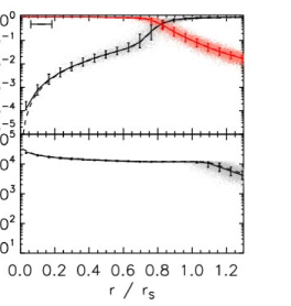
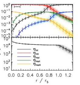
Figure 9: Test 2 (using traphic). Multi-frequency transport and effects of the inclusion of helium (Sec 5.3.2). Scatter plots and profiles of species fractions and temperature at time $t=100~{}\mbox{Myr}$. The left and right panels show, respectively, results from simulations of an ionising source in gas of pure hydrogen ($X=1$) and gas with primordial abundances ($X=0.75$, $Y=1-X$). Except for this difference in the helium abundance, both simulations are identical; in particular, they both make use of five frequency bins to transport the emitted $10^{5}~{}\mbox{K}$ blackbody photons. The panels could be compared with the left-most panels of Fig. 7, which show results from a simulation that is identical except that it used a single frequency bin and the grey, optically thin approximation. As in Fig. 7, each dot represents the species fraction (grey: $\eta_{\rm HI}$, red: $\eta_{\rm HII}$, blue: $\eta_{\rm HeI}$, green: $\eta_{\rm HeII}$, yellow: $\eta_{\rm HeIII})$ or temperature of a single SPH particle (only a randomly chosen subset of $10\%$ of all particles is shown). Solid curves show the median neutral fraction (ionised fraction, temperature) in spherical bins around the ionising source. The vertical error bars enclose $68.3\%$ of the particles in each bin. Dashed curves indicate the reference solution obtained with our 1-d RT code tt1d. The horizontal error bars in the upper left corners indicate the spatial resolution $\langle 2\tilde{h}\rangle$.

5.4 Test 3: Cosmological reionisation

In this section we use our thermally coupled implementation of traphic to repeat Test 4 of the cosmological RT code comparison project (Iliev et al., 2006a) that we have discussed in Paper I for the case of fixed temperature ($T=10^{4}~{}\mbox{K}$). This test involves the simulation of the evolution of ionised regions around multiple sources in a static cosmological density field at redshift $z\approx 8.85$ and was designed to resemble important aspects of state-of-the-art simulations of the epoch of reionisation. In contrast to our Test 4 simulations in Paper I, we will here compute the evolution of the temperature along with that of the ionisation state of the gas. We will perform both simulations assuming the grey approximations (optically thin and optically thick) and using multiple frequency bins and we will discuss the origin of the differences in the results that these simulations yield.

The setup of this test is identical to that of Test 4 in Paper I, to which we refer the reader for a detailed description. Briefly, the initial conditions are provided by a snapshot (at redshift $z\approx 8.85$) from a cosmological N-body and gas-dynamical uniform-mesh simulation. The simulation box is $L_{\rm box}=0.5~{}h^{-1}~{}\mbox{comoving Mpc}$ on a side, uniformly divided into $N_{\rm cell}=128^{3}$ cells. We Monte Carlo sample this input density field to replace the mesh cells with $N_{\rm SPH}=N_{\rm cell}=128^{3}$ SPH particles. The gas is assumed to be initially fully neutral and to have an initial temperature of $T=10^{2}~{}\mbox{K}$. The ionising sources are chosen to correspond to the 16 most massive halos in the box. They are assumed to have blackbody spectra $B_{\nu}(\nu,T_{\rm bb})$ with temperature $T_{\rm bb}=10^{5}~{}\mbox{K}$. The ionising photon production rate is taken to be constant and all sources are switched on at the same time. The box boundaries are photon-transmissive.

We perform three RT simulations to solve the time-independent RT equation, all with an angular resolution of $N_{\rm c}=32$ (and setting $\tilde{N}_{\rm ngb}=32$). We have demonstrated in Paper I (Test 4) that for the current problem this angular resolution is sufficiently high to obtain converged results. To facilitate a direct comparison with the corresponding simulation in Paper I, we employ the same time step $\Delta t_{\rm r}=10^{-4}~{}\mbox{Myr}$ and transport photons only over a single inter-particle distance per time step. We note that the current simulations do not employ the resampling technique to suppress noise in the neutral fraction caused by the particular realisation of the SPH density field. As discussed in Paper I, for the present test this noise is small. For definiteness we mention that all simulations include collisional ionisation and all relevant cooling processes (including Compton cooling off the $z=8.85$ cosmic microwave background), employing the rates listed in Table 1.

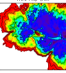
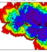
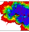
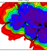
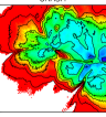
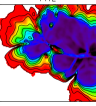
Figure 10: Test 3. Neutral fraction in a slice through $z=L_{\rm box}/2$ at time $t=0.2~{}\mbox{Myr}$. From left to right: traphic thin (assuming grey optically thin photoheating rates), traphic thick (assuming grey optically thick photoheating rates), traphic (using three frequency bins), c²-ray, crash and ftte. Contours show neutral hydrogen fractions $\eta_{\rm HI}=0.9,0.5$, $\log\eta_{\rm HI}=-1,-3$ and $-5$, from the outside in. The results obtained with traphic thick are in excellent agreement with those obtained with ftte. They are also in excellent agreement with the results obtained with c²-ray in highly ionised regions, where the neutral fraction is unaffected by spectral hardening. The small differences in the neutral fractions obtained with traphic thick, traphic thin and traphic are mostly due to differences in the recombination rate, caused by differences in the gas temperatures (see Fig. 11).

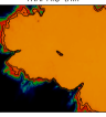
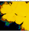
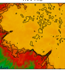
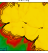
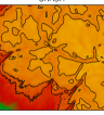
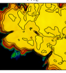
Figure 11: Test 3. Temperature in a slice through $z=L_{\rm box}/2$ at time $t=0.2~{}\mbox{Myr}$. From left to right: traphic thin (assuming optically thin photoheating rates), traphic thick (assuming optically thick photoheating rates), traphic (using three frequency bins), c²-ray, crash and ftte. Contours show temperatures $\log_{10}(T/{\rm K})=3,4,4.2,4.4$ and $4.6$, from the outside in. Most of the morphological differences may be attributed to differences in the spectral hardening of the ionising radiation, with the multi-frequency codes traphic, c²-ray and crash yielding a substantial amount of pre-heating and the monochromatic (grey) codes traphic thin, traphic thick and ftte yielding sharp transitions between the hot ionised and the cold neutral phases. The differences in the maximum gas temperatures are mainly due to photoheating being computed in the optically thick limit (traphic thick, c²-ray, ftte), the optically thin limit (traphic thin) or using multiple frequency bins (traphic, crash).

In the first two of the three simulations we transport radiation using a single frequency bin, employing the grey photoionisation cross-section $\langle\sigma_{\gamma\rm HI}\rangle=1.63\times 10^{-18}~{}\mbox{cm}^{2}$ (Sec. 3.1). The difference between these two simulations is in the computation of the photoheating rates used to evolve the gas temperatures. For one simulation (traphic thin) we compute photoheating in the optically thin limit, assuming that each photoionisation adds $\langle\epsilon_{\rm HI}\rangle=6.32~{}\mbox{eV}$ to the thermal energy of the gas (Sec. 3.2). In the other simulation (traphic thick) we compute photoheating in the optically thick limit, assuming that each photoionisation on average adds $\langle\epsilon^{\rm thick}_{\rm HI}\rangle=16.01~{}\mbox{eV}$ to the thermal energy of the gas (Sec. 3.2).

The third simulation (traphic) differs from the first two in that we transport photons using $N_{\nu}=3$ frequency bins (starting at $13.6~{}\mbox{eV}$, $35~{}\mbox{eV}$ and $50~{}\mbox{eV}$, with the last bin extending to infinity). The photoionisation cross-section and the excess energy associated with each bin are obtained from averaging over a blackbody spectrum of temperature $10^{5}~{}\mbox{K}$, assuming the optically thin limit (Eqs. 9 and 16). As in the previous section, our choice in favour of a very small number of frequency bins has purely practical reasons: computational efficiency. While we could have performed this relatively small test simulation at higher spectral resolution, we anticipate that applications of traphic to large simulations of reionisation will generally require us to choose a number of frequency bins as small as possible. Using a small number of frequency bins in the present test should thus give results that more closely resemble the results of future, larger simulations.

Figs. 10-12 show our results. Fig. 10 shows images of the neutral fraction in slices through the centre of the simulation box at time $t=0.2~{}\mbox{Myr}$ (our conclusions also hold for other times). The individual panels show results obtained with traphic thin, traphic thick and traphic. For reference, we also show the results obtained with other RT codes for the same test problem as published in Iliev et al. (2006a). Neutral fraction contours are shown to facilitate the comparison. While the simulation with crash treated the present problem by performing a multi-frequency computation, the simulation with ftte, as our simulation traphic thick, solved it in the grey approximation using optically thick photoheating rates. Finally, c²-ray employed a hybrid method that treats the transport of radiation with multiple frequency bins but computes photoheating rates in the grey (optically thick) approximation.

The differences in the neutral fractions are generally small. The simulations that employ photoheating rates in the optically thick limit (ftte, c²-ray, traphic thick) yield smaller minimum neutral fractions than the simulations that compute photoheating rates in the optically thin limit (traphic thin) or using multiple frequency bins (crash, traphic). This is the result of lower recombination rates caused by the higher temperatures these simulations yield (see Fig. 11). The regions with low ionisation ($\eta_{\rm HI}>0.5$) found with traphic are slightly smaller than those found with c²-ray and crash, which indicates that three frequency bins are not sufficient for obtaining highly accurate multi-frequency solution. Still, the simulations with traphic seem to capture the main effects (see the discussion on pre-heating below).

Fig. 11 shows images of the gas temperature in slices through the centre of the simulation box that correspond to the images of the neutral fraction shown in Fig. 10. There are significant differences in both the morphologies of the photo-heated regions and the typical temperatures attained by the photoionised gas between the different simulations. Outside the ionisation fronts, these differences can mostly be attributed to differences in the spectral hardening of the ionising radiation. c²-ray, crash and traphic all yield a substantial pre-heating of the gas ahead of the ionisation fronts. This pre-heating is not seen in the simulations with traphic thin, traphic thick and ftte since they all assume the grey approximation. In Sec. 5.2.2 we have already discussed, for the same set of codes, the differences between a multi-frequency treatment and its grey approximations in idealised simulations of the evolution of a single, spherically symmetric, ionised region. The results here are in close qualitative agreement with that discussion.

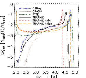
Figure 12: Test 3. Histograms of the temperature at time $t=0.2~{}\mbox{Myr}$ from simulations with different RT codes. At low temperatures the differences in the shapes of the histograms are mainly due to differences in the code-specific treatment of spectral hardening. The differences exhibited at high temperatures are mainly due to photoheating being computed in the optically thick limit (traphic thick, c²-ray, ftte), the optically thin limit (traphic thin) or using multiple frequency bins (crash, traphic).

The results obtained with the different codes also exhibit significant variations in the gas temperature in regions well inside the ionisation fronts. While crash, traphic and traphic thin yield typical temperatures of $T\approx 2-3\times 10^{4}~{}\mbox{K}$, the typical temperatures obtained with c²-ray, ftte and traphic thick are $T\approx 6\times 10^{4}~{}\mbox{K}$, i.e., substantially higher. Note that there is also disagreement between codes which incorporate the detailed treatment of multi-frequency radiation (c²-ray, crash, traphic) and between codes in which the radiation is treated in the grey approximation (ftte, traphic thin, traphic thick). Spectral hardening may thus only provide an explanation for part of the differences between the simulations.

We recall that in Sec. 5.2.2, where we simulated the evolution of a single, spherically symmetric, photoionised region, we found qualitatively similar differences between the results obtained with c²-ray, crash and ftte. In the (nearly optically thin) region close to the ionising source, the simulations that employed c²-ray and ftte yielded gas temperatures that were substantially larger than those in the simulation that employed crash. By comparing with results obtained with our 1-d RT code tt1d, we were able to explain most of these temperature differences in terms of differences in the assumptions underlying the computation of photoheating rates. The results presented in Fig. 11 are another manifestation of this explanation.

In Fig. 12 we compare histograms of the temperature at time $t=0.2~{}\mbox{Myr}$. For the simulations with c²-ray, crash and ftte we have computed these histograms directly from the $N_{\rm cell}=128^{3}$ values of temperatures published in Iliev et al. (2006a). For the simulations with traphic, traphic thin and traphic thick we assigned the temperatures to a corresponding uniform mesh with $N_{\rm cell}=128^{3}$ cells using SPH interpolation before we computed the histograms.

The histograms provide a quantitative confirmation of our qualitative discussion above. The simulations with traphic and traphic thin yield, in close agreement with the simulations performed with crash, typical temperatures of $T\approx 2-3\times 10^{4}~{}\mbox{K}$. On the other hand, the simulations performed with c²-ray, ftte and traphic thick closely agree on typical temperatures of $T\approx 6\times 10^{4}~{}\mbox{K}$. The differences between the histograms at low values of the temperature are mostly caused by the differences in spectral hardening. Due to the pre-heating of gas ahead of the ionisation fronts obtained with the multi-frequency codes traphic, c²-ray and crash, the number of cells that are still at their initial temperature $T=100~{}\mbox{K}$ is much smaller than found by ftte, traphic thin and traphic thick, which only employ a single frequency bin.

In summary, in this section we have repeated the simulation of the expansion of multiple ionised regions in a cosmological density field that we discussed in Test 4 in Paper I, but this time we explicitly computed the evolution of the temperature of the photoionised gas. We performed three simulations: one simulation computed photoheating in the grey, optically thin limit (traphic thin), one computed photoheating in the grey, optically thick limit (traphic thick) and one employed multiple (i.e., three) frequency bins. All three simulations showed only small differences in the neutral fractions when compared with each other, which could be plausibly explained with the differences in the temperatures. The temperatures differed due to the computation of photoheating rates in different limits (grey optically thin, grey optically thick and multi-frequency). In particular, employing the grey approximation in the optically thick limit yields temperatures that are typically too large by factors $2-3$. We also compared the results of our thermally coupled simulations with results obtained with other RT codes for the same test problem (Iliev et al., 2006a). We found very good agreement between these and our results when comparing simulations that employed similar assumptions for computing photoionisation and photoheating rates.

The results of the multi-frequency simulation (neutral fractions and temperatures interpolated to a $128^{3}$ uniform mesh using SPH interpolation) are available for download at the website of the Cosmological RT Code Comparison Project (Iliev et al., 2006a; Iliev et al., 2009).

6 Summary

In this work we described an extension of the implementation of traphic, the radiative transfer (RT) method for use with Smoothed Particle Hydrodynamics (SPH) simulations that we have introduced in Pawlik & Schaye (2008, Paper I), in a modified version of the SPH code gadget (Springel, 2005). The new implementation of traphic can be used to solve multi-frequency RT problems in primordial gas consisting of hydrogen and helium. It also allows for the computation of the non-equilibrium evolution of the gas temperature due to photoheating and radiative cooling.

As part of the new implementation we introduced a numerical method that allows us to accurately compute the coupled evolution of the ionisation balance and temperature of gas parcels exposed to ionising radiation and that works independently of the size of the chosen RT time step. This decoupling of the RT time step from the time scales that govern the evolution of the species fractions and temperatures, i.e. the decoupling from the ionisation, recombination and radiative cooling time scales, is an important pre-requisite for performing efficient RT simulations. The alternative, a RT time step limited by the values for the ionisation, recombination or cooling time scales, could quickly become computationally infeasible since these time scales may become very small.

We discussed the performance of the new, thermally coupled implementation of traphic in three-dimensional multi-frequency RT test simulations of spherically symmetric expanding HII regions and non-spherical expanding HII regions in a cosmological reionisation setting. We treated the multi-frequency radiation both using a single frequency bin in the grey approximation and using multiple frequency bins. We distinguished two types of grey approximations by computing photoheating both in the optically thin and optically thick limits. We compared the results of our test simulations to results obtained with other RT codes for identical test problems. We found excellent agreement in the morphologies and gas temperatures of the photoionised and photoheated regions when comparing simulations that employed similar assumptions for computing photoionisation and photoheating rates.

We used the new implementation to demonstrate and pinpoint the differences in the results obtained from grey simulations and simulations that use multiple frequency bins. Close to and ahead of ionisation fronts these differences are mostly due to the spectral hardening of the radiation field caused by the dependence of the absorption cross-section on photon energy. Spectral hardening significantly increases the widths of ionisation fronts and implies a substantial preheating of the gas ahead of them. Additional significant differences between the simulations are caused by the choice of the limit in which grey photoheating rates are computed. Simulations that use grey photoheating rates computed in the optically thick limit yield typical gas temperatures that are too large by factors $2-3$ when compared with the exact multi-frequency solution. Simulations that use grey photoheating rates computed in the optically thin limit yield typical gas temperatures that asymptote to the multi-frequency result with decreasing distances from the ionising sources.

The additions presented in this work are crucial for applications of traphic to simulations of the (re-)ionisation of both hydrogen and helium that also wish to account for the preheating of gas ahead of ionisation fronts due to spectral hardening. We plan to perform such simulations in the future. Note that we have limited our considerations to RT simulations on pre-computed static density fields. But photoheating increases also the gas pressure and hence affects the hydrodynamical evolution of the gas. An important goal for the future will therefore be to present an implementation of traphic that allows one to perform radiation-hydrodynamical simulations.

Appendix A A new treatment of absorptions by virtual particles

In this appendix we show that the treatment of virtual particles (ViPs) in the implementation of traphic that we have used to perform the (hydrogen-only) simulations published in Pawlik & Schaye (2008, hereafter Paper I) and that we will refer to as the old implementation, results in a temporary underestimate of the neutral hydrogen fraction just behind evolving ionisation fronts in simulations that use a high angular resolution. We will show that this underestimate is absent in simulations that employ our new implementation (presented in the current work). Moreover, in simulations that employ this new implementation, the numerical scatter in the neutral hydrogen fraction is significantly reduced. For clarity of the presentation and because we will compare results obtained with the new implementation with results obtained with the old implementation presented in Paper I that lacked the treatment of helium, we will assume that photons are transported in gas that consists only of hydrogen (i.e., $X=1$). Our discussion generalizes straightforwardly to the transport of photons in gas consisting of both hydrogen and helium.

The number of hydrogen-ionising photons a ViP absorbs depends on its neutral hydrogen density. As explained in Paper I, the computation of this number is performed in exactly the same manner as for SPH particles. The only difference between the treatment of photons absorbed by SPH particles and ViPs is that the latter distribute the absorbed photons amongst their SPH neighbours. For this distribution of absorbed photons one must specify the fraction of the total that is given to each of the SPH neighbours. In the old implementation of traphic  this fraction was taken to be proportional to the value of the SPH kernel $W$ of the distributing ViP at the position of the SPH neighbour. In the new version this fraction is taken to be proportional to the contribution of the SPH neighbour to the SPH estimate of the ViP’s neutral hydrogen density.

The old treatment of ViPs results in an underestimate of the simulated non-equilibrium neutral hydrogen fractions. Fig. 13 serves to demonstrate this. Its panels show the neutral and ionised hydrogen fractions around a single ionising source in a homogeneous hydrogen-only medium at times $t=30,100$ and $500~{}\mbox{Myr}$ (from left to right) obtained with the old (first and third rows) and new (second and fourth rows) implementation. The setup and parameters for the simulations presented here are identical to the setup and parameters used for the $N_{\rm SPH}=64^{3}$, $N_{\rm c}=128$ simulation presented in Test 1 in Sec. 5.3.1 of Paper I. In addition to the neutral (grey dots) and ionised (light red dots) fractions of each particle, Fig. 13 shows the median neutral (black solid curves) and ionised (red solid curves) fractions in spherical bins, which are compared to the exact solution obtained with our 1-d RT code tt1d (Sec. 5.3; dashed curves of the corresponding colour). The error bars indicate the $68.3\%$ confidence intervals in each bin. For each implementation we have performed simulations both with and without resampling the density field, as indicated by the presence or absence of the letter ‘R’ in the panel titles.

In the simulations employing the old implementation of traphic the neutral hydrogen fractions at times $t=30$ and $100~{}\mbox{Myr}$ are underestimated at radii slightly smaller than the radius of the ionisation front. In the simulations that employ the new implementation this underestimate is no longer present, thanks to the new manner in which the photons absorbed by ViPs are distributed. At $t=500~{}\mbox{Myr}$, i.e. when the ionised region has (nearly) reached its equilibrium size, the underestimate is also absent in the simulations that employ the old implementation. However, at this time these old simulations still exhibit an increased scatter around the median when compared to the corresponding snapshots from the simulations that employ the new implementation.

The underestimate of the neutral hydrogen fraction just behind evolving ionisation fronts in simulations employing the old implementation is caused by the fact that in this implementation the distribution of the photons absorbed by ViPs does not respect the spatial distribution of the neutral gas in their surroundings. It mainly affects the neutral fraction of particles close to evolving ionisation fronts, because the number of photons absorbed and subsequently distributed by ViPs near the ionisation front is significantly larger than the number of photons that are absorbed by the SPH particles behind the ionisation front and because the ViPs distribute the absorbed photons irrespective of the neutral hydrogen mass with which the corresponding SPH particles contributed to the computation of its neutral hydrogen density.

We did not notice the described temporary underestimate of the neutral fraction just behind non-equilibrium ionisation fronts in the simulations that we have presented in our original publication (Paper I), since there we only discussed profiles of the neutral fraction at $t=500~{}\mbox{Myr}$. The reason why we limited ourselves to discussion of equilibrium results in that publication, was that we were still lacking accurate non-equilibrium reference solutions at that time (our 1-d reference RT code tt1d was still under development). The discovery of the underestimate of the neutral fraction was triggered by scatter plots of the neutral and ionised hydrogen fractions like those presented in Fig. 13 that we have performed more recently.

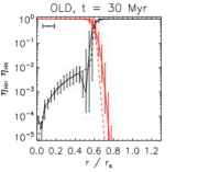
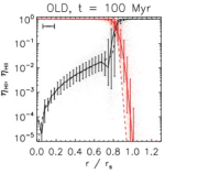
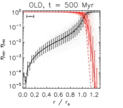
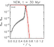
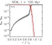
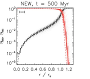
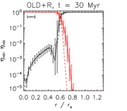
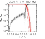
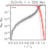
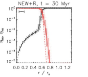
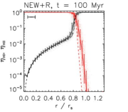
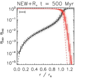
Figure 13: Test 1. Neutral and ionised hydrogen fractions obtained in simulations with the old (Pawlik & Schaye, 2008; first and third row) and new (second and fourth row) implementations of traphic. Shown are profiles of neutral and ionised fractions at times $t=30$ (left panel), $100$ (middle panel) and $500~{}\mbox{Myr}$ (right panel), for simulations with (second and fourth row) and without (first and third row) resampling of the density field. The spatial resolution is fixed to $N_{\rm SPH}=64^{3}$, $\tilde{N}_{\rm ngb}=32$ and is indicated by the horizontal error bar in the upper left corner of each panel. The angular resolution is $N_{\rm c}=128$. The grey (light red) points show the neutral (ionised) hydrogen fraction for a randomly chosen subset of $10\%$ of all particles. The solid black (red) curve shows the median neutral (ionised) hydrogen fraction in spherical bins and the error bars enclose $68.3\%$ of the particles in each bin. The dashed black (red) curves show the exact solutions, obtained with our reference code tt1d. The underestimate of the non-equilibrium neutral fraction exhibited in simulations with the old implementation of traphic is absent in the simulations that employ our new implementation, thanks to a new self-consistent manner of distributing photons absorbed by ViPs. The new implementation also reduces the scatter in the ionisation balance.

References

- Abel & Haehnelt (1999) Abel, T., Haehnelt, M. G., 1999, ApJL, 520, L13
- Abel, Norman, & Madau (1999) Abel T., Norman M. L., Madau P., 1999, ApJ, 523, 66
- Aldrovandi & Pequignot (1973) Aldrovandi S. M. V., Pequignot D., 1973, A&A, 25, 137
- Altay, Croft, & Pelupessy (2008) Altay G., Croft R. A. C., Pelupessy I., 2008, MNRAS, 386, 1931
- Aubert & Teyssier (2008) Aubert D., Teyssier R., 2008, MNRAS, 387, 295
- Badnell (2001) Badnell N. R., 2001, ASPC, 247, 37
- Barkana & Loeb (2001) Barkana R., Loeb A., 2001, PhR, 349, 125
- Black (1981) Black J. H., 1981, MNRAS, 197, 553
- Bolton, Meiksin, & White (2004) Bolton J., Meiksin A., White M., 2004, MNRAS, 348, L43
- Cantalupo & Porciani (2010) Cantalupo S., Porciani C., 2010, arXiv, arXiv:1009.1625
- Cen (1992) Cen R., 1992, ApJS, 78, 341
- Ciardi et al. (2001) Ciardi B., Ferrara A., Marri S., Raimondo G., 2001, MNRAS, 324, 381
- Ciardi & Ferrara (2005) Ciardi B., Ferrara A., 2005, SSRv, 116, 625
- Dove & Shull (1994) Dove J. B., Shull J. M., 1994, ApJ, 430, 222
- Fan, Carilli, & Keating (2006) Fan X., Carilli C. L., Keating B., 2006, ARA&A, 44, 415
- Ferland et al. (1998) Ferland G. J., Korista K. T., Verner D. A., Ferguson J. W., Kingdon J. B., Verner E. M., 1998, PASP, 110, 761
- Furlanetto, Oh, & Briggs (2006) Furlanetto S. R., Oh S. P., Briggs F. H., 2006, PhR, 433, 181
- Furlanetto & Stoever (2010) Furlanetto S. R., Stoever S. J., 2010, MNRAS, 404, 1869
- Finlator, Özel, & Davé (2009) Finlator K., Özel F., Davé R., 2009, MNRAS, 393, 1090
- Gingold & Monaghan (1977) Gingold R. A., Monaghan J. J., 1977, MNRAS, 181, 375
- Gnedin (2000) Gnedin N. Y., 2000, ApJ, 542, 535
- Gnedin & Abel (2001) Gnedin N. Y., Abel T., 2001, NewA, 6, 437
- Gritschneder et al. (2009) Gritschneder M., Naab T., Burkert A., Walch S., Heitsch F., Wetzstein M., 2009, MNRAS, 393, 21
- Hasegawa & Umemura (2010) Hasegawa, K., & Umemura, M. 2010, arXiv:1005.5312
- Hui & Gnedin (1997) Hui L., Gnedin N. Y., 1997, MNRAS, 292, 27
- Hummer & Storey (1998) Hummer D. G., Storey P. J., 1998, MNRAS, 297, 1073
- Iliev et al. (2006a) Iliev I. T., et al., 2006a, MNRAS, 371, 1057
- Iliev et al. (2006b) Iliev I. T., Mellema G., Pen U.-L., Merz H., Shapiro P. R., Alvarez M. A., 2006b, MNRAS, 369, 1625
- Iliev et al. (2009) Iliev I. T., et al., 2009, MNRAS, 400, 1283
- Lucy (1977) Lucy L. B., 1977, AJ, 82, 1013
- Madau & Efstathiou (1999) Madau P., Efstathiou G., 1999, ApJ, 517, L9
- Maselli, Ferrara, & Ciardi (2003) Maselli A., Ferrara A., Ciardi B., 2003, MNRAS, 345, 379
- Maselli, Ciardi, & Kanekar (2009) Maselli A., Ciardi B., Kanekar A., 2009, MNRAS, 393, 171
- Mellema et al. (2006) Mellema G., Iliev I. T., Alvarez M. A., Shapiro P. R., 2006, NewA, 11, 374
- Mihalas & Weibel Mihalas (1984) Mihalas, D., Weibel Mihalas, B., 1984, Foundations of radiation hydrodynamics, Oxford University Press, New York
- Nakamoto, Umemura, & Susa (2001) Nakamoto T., Umemura M., Susa H., 2001, MNRAS, 321, 593
- Monaghan (2005) Monaghan J. J., Rep. Prog. Phys., 68, 1703 (2005)
- McQuinn et al. (2007) McQuinn M., Lidz A., Zahn O., Dutta S., Hernquist L., Zaldarriaga M., 2007, MNRAS, 377, 1043
- McQuinn et al. (2009) McQuinn M., Lidz A., Zaldarriaga M., Hernquist L., Hopkins P. F., Dutta S., Faucher-Giguère C.-A., 2009, ApJ, 694, 842
- Osterbrock (1989) Osterbrock D. E., 1989, Astrophysics of gaseous nebulae and active galactic nuclei, Palgrave Macmillan
- Paardekooper, Kruip, & Icke (2010) Paardekooper J.-P., Kruip C. J. H., Icke V., 2010, A&A, 515, A79
- Partl et al. (2010) Partl A. M., Dall’Aglio A., Müller V., Hensler G., 2010, arXiv, arXiv:1009.3424
- Pawlik & Schaye (2008) Pawlik A. H., Schaye J., 2008, MNRAS, 389, 651
- Pawlik (2009) Pawlik A. H., 2009, PhD Thesis, Leiden University (http://hdl.handle.net/1887/14025)
- Petkova & Springel (2009) Petkova M., Springel V., 2009, MNRAS, 396, 1383
- Press et al. (1992) Press W. H., Teukolsky S. A., Vetterling W. T., Flannery B. P., 1992, Numerical recipes in C. The art of scientific computing, Cambridge University Press, 2nd ed.
- Razoumov & Cardall (2005) Razoumov A. O., Cardall C. Y., 2005, MNRAS, 362, 1413
- Ritzerveld (2005) Ritzerveld J., 2005, A&A, 439, L23
- Ritzerveld & Icke (2006) Ritzerveld J., Icke V., 2006, PhRvE, 74, 026704
- Savin (2000) Savin D. W., 2000, ApJ, 533, 106
- Semelin, Combes, & Baek (2007) Semelin B., Combes F., Baek S., 2007, A&A, 474, 365
- Shampine & Gear (1979) Shampine L. F., Gear C. W., 1979, SIAM Review, Vol. 21, No. 1., pp. 1-17, Jstor.
- Shapiro & Kang (1987) Shapiro P. R., Kang H., 1987, ApJ, 318, 32
- Shull & van Steenberg (1985) Shull J. M., van Steenberg M. E., 1985, ApJ, 298, 268
- Spitzer (1978) Spitzer L., 1978, Physical processes in the interstellar medium, New York Wiley-Interscience
- Springel (2005) Springel V., 2005, MNRAS, 364, 1105
- Springel (2010) Springel V., 2010, ARA&A, 48.
- Susa (2006) Susa H., 2006, PASJ, 58, 445
- Theuns et al. (1998) Theuns T., Leonard A., Efstathiou G., Pearce F. R., Thomas P. A., 1998, MNRAS, 301, 478
- Trac & Cen (2007) Trac H., Cen R., 2007, ApJ, 671, 1
- Verner et al. (1996) Verner D. A., Ferland G. J., Korista K. T., Yakovlev D. G., 1996, ApJ, 465, 487
- Whalen & Norman (2008) Whalen D., Norman M. L., 2008, ApJ, 673, 664
- White (1996) White S. D. M., 1996, Cosmology and large scale structure, Proceedings of the ”Les Houches Ecole d’Ete de Physique Theorique” (Les Houches Summer School), p. 349, Elsevier Scientific Publishing Company, Amsterdam
- Williams & Henney (2009) Williams R. J. R., Henney W. J., 2009, MNRAS, 400, 263
- Zahn et al. (2010) Zahn O., Mesinger A., McQuinn M., Trac H., Cen R., Hernquist L. E., 2010, arXiv, arXiv:1003.3455