A SEMI-EMPIRICAL MASS-LOSS RATE IN SHORT-PERIOD CATACLYSMIC VARIABLES

Abstract

The mass-loss rate of donor stars in cataclysmic variables (CVs) is of paramount importance in the evolution of short-period CVs. Observed donors are oversized in comparison with those of isolated single stars of the same mass, which is thought to be a consequence of the mass loss. Using the empirical mass-radius relation of CVs and the homologous approximation for changes in effective temperature $T_{2}$, orbital period $P$, and luminosity of the donor with the stellar radius, we find the semi-empirical mass-loss rate ${\dot{M}_{2}}$ of CVs as a function of $P$. The derived ${\dot{M}_{2}}$ is at $\sim 10^{-9.5}$–$10^{-10}$ ${\rm\;M_{\odot}\;\rm yr^{-1}}$ and depends weakly on $P$ when $P>90$ min, while it declines very rapidly towards the minimum period when $P<90$ min, emulating the $P$–$T_{2}$ relation. Due to strong deviation from thermal equilibrium caused by the mass loss, the semi-empirical ${\dot{M}_{2}}$ is significantly different from, and has a less-pronounced turnaround behavior with $P$ than suggested by previous numerical models. The semi-empirical $P$–${\dot{M}_{2}}$ relation is consistent with the angular momentum loss due to gravitational wave emission, and strongly suggests that CV secondaries with $0.075{\rm\;M_{\odot}}<M_{2}<0.2{\rm\;M_{\odot}}$ are less than 2 Gyrs old. When applied to selected eclipsing CVs, our semi-empirical mass-loss rates are in good agreement with the accretion rates derived from the effective temperatures $T_{1}$ of white dwarfs, suggesting that ${\dot{M}_{2}}$ can be used to reliably infer $T_{2}$ from $T_{1}$. Based on the semi-empirical ${\dot{M}_{2}}$, SDSS 1501 and 1433 systems that were previously identified as post-bounce CVs have yet to reach the minimal period.

1 Introduction

Cataclysmic variables (CVs) are semi-detached binaries with a white dwarf (WD) primary and a low-mass companion which transfers mass to a WD through Roche-lobe overflow. The observed orbital period distribution of CVs has three important features: a sharp short period cut-off at the orbital period of ${P_{\rm min}}\simeq 76.2$ min, referred to as the “minimum period”, the period gap, a dearth of systems with periods between ${P_{\rm gap}^{~{}-}}\simeq 129$ min and ${P_{\rm gap}^{~{}+}}\simeq 192$ min (Knigge, 2006), and the “period minimum spike”, a significant accumulation of systems at $P\sim 80$–$86$ min (Gånsicke et al., 2009). For CVs with period above ${P_{\rm gap}^{~{}+}}$, the dominant angular momentum loss mechanism is thought to be the magnetic braking, while the gravitational radiation may be responsible for the angular momentum loss for CVs below ${P_{\rm gap}^{~{}-}}$. In this work, we focus on CVs only with $P<{P_{\rm gap}^{~{}-}}$.

A characteristic feature of CVs is the mass transfer from a secondary to a WD. Since the gas stream carries substantial angular momentum, it forms an accretion disk around the WD. The reaction of a CV on the mass transfer can be qualitatively understood with the help of the dimensionless parameter

$$\tau=\frac{{\tau_{\rm M}}}{{\tau_{\rm KH}}},$$ (1)

where ${\tau_{\rm M}}$ and ${\tau_{\rm KH}}$ denote the mass-loss and Kelvin-Helmholtz timescales of the donor, respectively (Paczynski, 1981). At the initial phase of mass transfer, $\tau\gg 1$, so that the donor remains close to thermal equilibrium and thus follows the mass-radius relation (MRR) of main-sequence stars

$$R_{2}\propto M_{2}^{\xi_{\rm E}},$$ (2)

with the effective mass-radius exponent ${\xi_{\rm E}}$ close to $0.64^{+0.02}_{-0.02}$ (Knigge, 2006). Here, the subscript “2” denotes the quantities of CV donors. Both $R_{2}$ and $P$ of the CV decrease as the donor keeps losing mass during this early phase of CV evolution.

As the mass transfer continues, the binary shrinks due to the angular momentum loss, reducing $\tau$. When ${\tau_{\rm M}}$ and ${\tau_{\rm KH}}$ become comparable to each other ($\tau\approx 1$), the donor becomes out of thermal equilibrium. Since the surface luminosity is no longer in balance with the nuclear luminosity, the donor expands, causing ${\xi_{\rm E}}$ to decrease with time (King, 1988). Using the Hayashi theory and homologous approximation, Stehle et al. (1996) studied the reaction of the donor to mass loss and found that $R_{2}$ increases with decreasing $\tau$. Observations confirm this theoretical prediction, showing that the radii of donors in short-period CVs are $\sim 5$–$50\%$ larger than those of isolated main-sequence stars (Patterson et al., 2005; Knigge, 2006).

The effective mass-radius exponent ${\xi_{\rm E}}$ becomes smaller as $M_{2}$ decreases towards the brawn dwarfs masses. The change in the MRR of donors slows down the temporal change in the orbital period as the donor continues losing mass. The orbital period reaches a minimum value when ${\xi_{\rm E}}\approx 1/3$ at which $dP/dM_{2}=0$ (Rappaport et al., 1982). As $\tau$ decreases further, ${\xi_{\rm E}}$ declines to $0.21^{+0.05}_{-0.10}$ (Knigge, 2006). This in turn leads to an increase in $P$. Such a turnaround of the orbital period at ${P_{\rm turn}}$ is referred to as the “period bounce”.

The evolutionary scenario described above suggests that the mass-loss rates ${\dot{M}_{2}}$ (and the related thermal relaxation) of donors control the evolution of CVs. It also implies that the observed distribution of CVs versus the orbital period may be a consequence of a certain relation between ${\dot{M}_{2}}$ and $P$. Since ${\dot{M}_{2}}(P)$ not only provides a way to estimate the ages of CVs but also can be used to check the dominant mechanism for angular momentum loss, finding a reliable $P$–${\dot{M}_{2}}$ relationship is of great importance in understanding CV evolution.

There have been numerous studies to derive the $P$–${\dot{M}_{2}}$ relation; these can be categorized into two groups: purely theoretical work (e.g., Rappaport et al. 1982; Ritter 1988; King 1988; Kolb & Baraffe 1999; Howell et al. 2001) and semi-empirical work (e.g., Patterson 1984; Urban & Sion 2006; Townsley & Gånsicke 2009). The first, theoretical studies made use of stellar evolution codes combined with the analytical mass-transfer models of Ritter (1988) or others. The common results of these numerical experiments are that (1) the orbital period exhibits the turnaround behavior at ${P_{\rm turn}}$ that is about $\sim 10\%$ smaller than the observed ${P_{\rm min}}$ (Rappaport et al., 1982; Kolb & Baraffe, 1999; Howell et al., 2001) and (2) compared to isolated stars, the secondaries in short-period CVs are oversized due to the mass loss but only by $\sim 5$–$20\%$, which is about a factor $\sim 1.5$–$2$ smaller than the observed CV sizes. Since the bloating of the donor depends on the efficiency of the mass loss, these results suggest either the numerical models underestimate ${\dot{M}_{2}}$ above ${P_{\rm turn}}$, or the efficiency of the angular momentum loss is higher than expected (Kolb & Baraffe, 1999; Renvoizé et al., 2002). Despite the attempts to include the effects of tidal and rotational perturbations (Rezzolla et. al., 2001; Renvoizé et al., 2002; Kolb & Baraffe, 1999), additional angular momentum loss via magnetic braking (Andronov et al., 2003), accretion disk winds and magnetic propeller (see Barker 2003 for review), etc., clear explanations for the discrepancies between ${P_{\rm turn}}$ and ${P_{\rm min}}$ and between the empirical and numerical MRRs have yet to be found.

The second, semi-empirical approach uses, for instance, the effective temperatures of WDs (Townsley & Bildsten, 2003, 2004; Townsley & Gånsicke, 2009) or accretion disk luminosities (Patterson, 1984) to infer the accretion rates ${\dot{M}_{1}}$. The physical basis for the former is that WDs in CVs are observed to be hotter than expected from their ages (Sion, 1995), and such “overheating” of WDs may be a result of the compressional heating due to the gas piled up on their surfaces (Townsley & Bildsten, 2003). For the latter method, the accretion luminosities can give direct information on ${\dot{M}_{1}}$ if the disk properties are well constrained. When applied to dwarf novae (DNe) that accrete sporadically and have thermally unstable disks, ${\dot{M}_{1}}$ calculated from the two methods have a different scatter for given $P$. The mass-transfer rates based on the accretion luminosities probably measure an accretion rate averaged over short time intervals, e.g., a few decades, which makes them quite sensitive to short-time disk variability (Townsley & Gånsicke, 2009). This inevitably leads to a high dispersion in ${\dot{M}_{1}}$ estimated from the disk luminosities. On the other hand, the effective temperatures of WDs are likely to give a relatively long-term averaged ${\dot{M}_{1}}$, although this method may suffer from uncertainties related to unknown properties such as masses and radii of WDs as well as some auxiliary assumptions on their structures and boundary layers (Patterson, 2009).

In this paper we construct another semi-empirical relation between the mass-loss rate and the orbital period, and compare the result with those of the purely theoretical and the semi-empirical approaches mentioned above. We start from the empirical MRR of Knigge (2006) for superhumping CVs, and apply the homologous approximation in order to calculate the dependencies of the effective temperature and gravothermal luminosity upon the bloating of the donor. Assuming that the observed MRR of CV donors is a consequence of the mass loss and thermal relaxation processes, we calculate the mass-loss rates. We will show that the resulting mass-loss rates are broadly in line with those on the basis of the effective temperatures of WDs, while different from those of the purely theoretical models of Kolb & Baraffe (1999). We will also show that our results are consistent with the angular momentum loss of CVs due primarily to the emission of gravitational waves. Since radii of CV donors likely trace the long-term evolution of ${\dot{M}_{2}}$ (Knigge, 2006) and depend only weakly on details of the mass-transfer processes, the resulting mass-loss rates from the empirical MRR are less model-dependent and less sensitive to the short-term effects than the other semi-empirical estimates that rely on accretion activities.

The organization of this paper is as follows. In §2, we introduce the theoretical MRR for isolated single stars and the empirical MRR for CVs donors, and define the bloating factor. We then describe a method to find the effective temperature and gravothermal luminosity of donors by using the bloating factor. In §3, we calculate the semi-empirical mass-loss rate, construct the mass-loss history to estimate the CV ages, and show that the derived mass-loss rate is consistent with CV evolution by angular momentum loss via the emission of gravitational waves. In §4, we apply our results to selected eclipsing short-period CVs and show that the semi-empirical mass-loss rate is consistent with the accretion rates inferred from the effective temperatures of WDs. We also suggest a way to estimate the effective temperatures of donors assuming that mass is conserved. Finally, we summarize our results in §5.

2 Mass-radius and Period-effective Temperature Relations

We consider a CV consisting of a WD (or accretor) with mass $M_{1}$ and a secondary (or donor) with mass $M_{2}$, radius $R_{2}$, and effective temperature $T_{2}$. We assume that the donor fills its critical equipotential surface. In accordance with the results of Patterson et al. (2005) and Knigge (2006), we assume $M_{1}=0.75{\rm\;M_{\odot}}$ throughout this paper. We use an additional subscript “0” to denote the quantities of isolated, single stars in hydrostatic and thermal equilibrium to which CV secondaries will be compared. In this section, we use the empirical relationship between masses and radii of CV secondaries to calculate the bloating factor in comparison with the single stars of the same mass. We then treat the bloating factor as perturbations to the properties of single stars in order to find the orbital period, effective temperature, and gravothermal luminosity of CVs.

2.1 Mass-radius Relations

As the MRRs of single stars that we use as the references to those of CV secondaries, we take composite relations constructed in a manner similar to Knigge (2006): the BCAH98 isochrone of Baraffe et al. (1998) for stars with $0.075{\rm\;M_{\odot}}\leq M_{2}<0.3{\rm\;M_{\odot}}$, the DUSTY isochrone of Baraffe et al. (2002) for $0.06{\rm\;M_{\odot}}\leq M_{2}<0.075{\rm\;M_{\odot}}$ ($1500\lesssim T_{2}\lesssim 2000$ K), and the COND isochrone of Baraffe et al. (2003) for $M_{2}<0.06{\rm\;M_{\odot}}$.

There are quite large uncertainties in the estimation of CV ages. Period bouncers are thought of as a final stage of CV evolution, suggesting that they are older than their “parent” CVs (see, e.g., Paczynski 1981; Rappaport et al. 1982; Kolb & Baraffe 1999). Although numerical experiments predict that CVs cross the period gap at $\sim 1$ Gyr and reach ${P_{\rm turn}}$ in $\sim 4$ Gyr after the onset of the mass loss below the gap (e.g., Kolb & Baraffe 1999; Howell et al. 2001), temporal evolution of CVs depends strongly on the mass-loss rate that is not well constrained observationally. To cover a wide range of CV ages, we adopt two composite isochrones with 1-Gyr and 5-Gyr ages (hereafter B1 and B5 sequences, respectively). Figure 1 plots the composite $R_{2,0}$ of single stars as functions of $M_{2}$ for the B1 and B5 sequences, as dashed and solid lines, respectively. Both sequences give almost the same radii above ${0.075\rm\;M_{\odot}}$, while below this point the stellar radii in the B1 sequence are about $\sim 10\%$ larger than in the B5 sequence.

As the MRR of CV secondaries, we take the relation derived by Knigge (2006) from the observed properties of superhumping CVs:

$$\frac{R_{2}}{{\rm\;R_{\odot}}}=\begin{cases}0.110\bigl{(}\frac{M_{2}}{0.063{\rm\;M_{\odot}}}\bigr{)}^{0.21},&\;\;0.063{\rm\;M_{\odot}}<M_{2},\\ 0.230\bigl{(}\frac{M_{2}}{0.2{\rm\;M_{\odot}}}\bigr{)}^{0.64},&\;\;0.063{\rm\;M_{\odot}}\leq M_{2}<0.2{\rm\;M_{\odot}},\\ 0.299\bigl{(}\frac{M_{2}}{0.2{\rm\;M_{\odot}}}\bigr{)}^{0.67},&\;\;0.2{\rm\;M_{\odot}}\leq M_{2}.\end{cases}$$ (3)

This empirical fit assumes $M_{1}=0.75{\rm\;M_{\odot}}$ and incorporates itself the additional empirical constraints that reproduce the observed locations of the period gap and the period minimum, such that ${P_{\rm gap}^{~{}-}}$ occurs at $M_{2}=0.2\pm{0.02}{\rm\;M_{\odot}}$ and ${P_{\rm min}}$ at $M_{2}=0.063\pm{0.009}{\rm\;M_{\odot}}$. The intrinsic errors in $R_{2}$ for this empirical MRR are estimated to be about $2$–$3\%$ (Knigge, 2006); we take allowance for $4\%$ uncertainties in $R_{2}$ throughout this work. We note a caveat that our choice of the errors may underestimate real values below ${0.075\rm\;M_{\odot}}$ where only a few systems are observed and thus there is practically no calibrator. In addition, the masses of WDs may differ from the assumed mass of $0.75{\rm\;M_{\odot}}$, which also can change $R_{2}$. Equation (3) is plotted in Figure 1 as dotted line with the shaded region denoting the associated uncertainties in $R_{2}$. Columns (1) and (2) in Table 1 give the $M_{2}$-$R_{2}$ relation.

For comparison, Figure 1 also plots as a dot-dashed line the MRR of CVs with $0.03{\rm\;M_{\odot}}<M_{2}<0.21{\rm\;M_{\odot}}$ from the numerical models of Kolb & Baraffe (1999), which clearly has smaller radii than the empirical relation, typically by $\sim 5$–$10\%$. This indicates that the deviation of real donors from thermal equilibrium is larger than that expected from the numerical models.

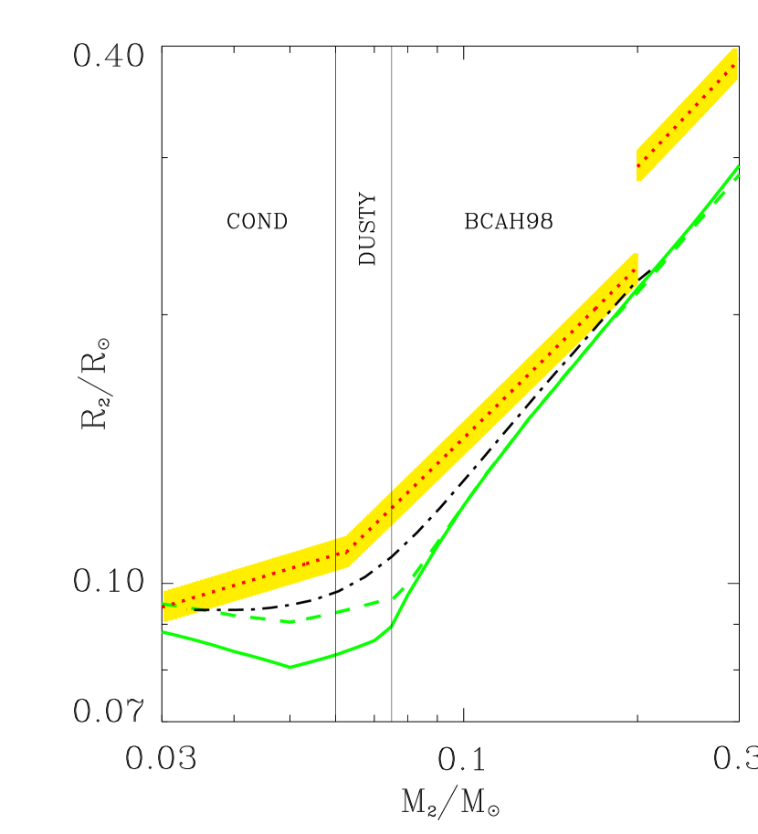
Figure 1: Mass-radius relations of CV donor stars. The dotted line plots the empirical MRR from Knigge (2006) with the 4% uncertainties indicated by the shaded region. The dashed and solid lines represent the unperturbed MRR of singles stars for the B1 and B5 sequences, respectively. The dot-dashed line is for the MRR of evolving donors from the numerical models of Kolb & Baraffe (1999). The thin vertical lines mark the boundaries of the adopted isochrones: BCAH98 for $0.075\leq M_{2}<0.3{\rm\;M_{\odot}}$; DUSTY for $0.06\leq M_{2}<0.075{\rm\;M_{\odot}}$; COND for $M_{2}<0.06{\rm\;M_{\odot}}$.

2.2 Bloating Factor

We define the bloating factor

$$\alpha=\frac{R_{2}}{R_{2,0}},$$ (4)

as the relative size of a CV secondary to a single star with the same mass. Figure 2 plots $\alpha$ as dashed and solid lines for the B1 and B5 sequences, respectively, with the shaded and hatched regions representing the corresponding uncertainties. The discontinuity of $\alpha$ at $M_{2}=0.2{\rm\;M_{\odot}}$ corresponds to the period gap. Since $P\propto\alpha^{3/2}$ (see below), the ratio of the bloating factors above (${\alpha_{\rm gap}^{+}}$) and below (${\alpha_{\rm gap}^{-}}$) the gap satisfies ${\alpha_{\rm gap}^{+}}/{\alpha_{\rm gap}^{-}}=({P_{\rm gap}^{~{}+}}/{P_{\rm gap}^{~{}-}})^{2/3}=1.3$, in good agreement with the width of the gap. At the upper edge of the gap, the donors detach from their critical lobes and the mass loss stops. Since the donors are thought to be oversized due to the mass loss, they shrink within the gap. When the donors come out the lower edge of the gap, they resume the mass loss and become oversized again.

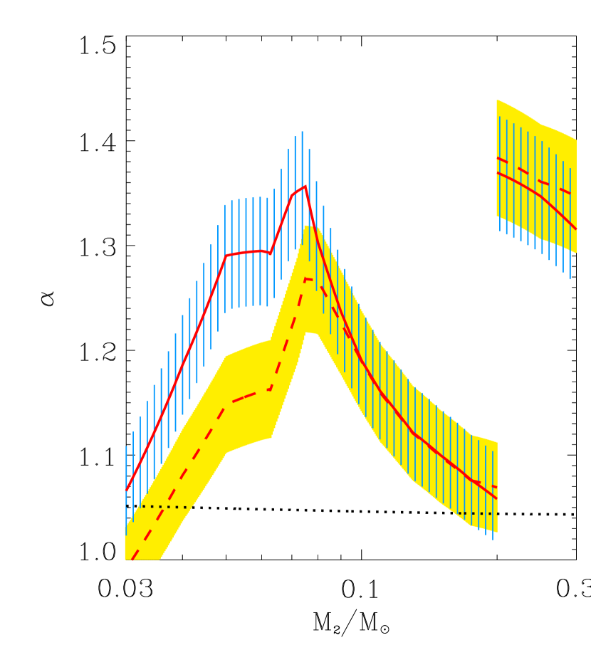
Figure 2: Bloating factors $\alpha$ of CV donors as functions of their mass $M_{2}$. The dashed and solid lines are for the B1 and B5 sequences, respectively, with the shaded and hatched regions corresponding to the uncertainties. The dotted line shows the bloating factor of Roche-lobe filling polytropes with $n=3/2$ due to the isentropic expansion caused by tidal and rotational perturbations, when its companion has a mass of $M_{1}=0.75{\rm\;M_{\odot}}$.

Figure 2 shows that the bloating factor increases with the decreasing donor mass for $M_{2}>{0.075\rm\;M_{\odot}}$ and then decreases with decreasing $M_{2}$ below this point. This can be explained qualitatively as follows. Since stars with $M_{2}<0.3{\rm\;M_{\odot}}$ are fully convective and isentropic, they are well described by polytropes with index $n=3/2$ (Burrows & Leibert, 1993). The MRR for these polytropes

$$R_{2}\propto KM_{2}^{-1/3},$$ (5)

with $K$ being the pressure constant (Chandrasekhar, 1939), then gives

$$\alpha=\frac{K}{K_{0}}.$$ (6)

The mass loss is capable of driving the donor out of thermal equilibrium. This raises the gravothermal luminosity, ${L_{\rm g}}=L_{2}-{L_{\rm nuc}}$, where ${L_{\rm nuc}}$ is the nuclear luminosity of the donor and $L_{2}$ is the surface luminosity. For fully convective stars, the change of $K$ depends on ${L_{\rm g}}$ and ${\tau_{\rm KH}}$ as

$$\frac{\dot{K}}{K}\propto-\frac{1}{{\tau_{\rm KH}}}\frac{{L_{\rm g}}}{L_{2}},$$ (7)

(King, 1988; Ritter, 1996). Combining equations (5), (6), and (7), one obtains

$$\frac{\dot{\alpha}}{\alpha}\propto-\frac{1}{{\tau_{\rm KH}}}\frac{{L_{\rm g}}}{L_{2}}+\frac{1}{{\tau_{\rm M}}}\biggl{(}{\xi_{\rm E}}_{0}+\frac{1}{3}\biggr{)},$$ (8)

where ${\xi_{\rm E}}_{0}$ is the mass-radius exponent of unperturbed, singe stars. At the lower edge of the period gap, a donor remains close to thermal equilibrium so that ${L_{\rm g}}\approx 0$ and ${\xi_{\rm E}}_{0}\approx 1$. In this case, the second term in the right-hand side of equation (8) dominates and $\dot{\alpha}/\alpha>0$, indicating that $\alpha$ increases as the mass loss continues. When the donor reaches the minimum hydrogen burning mass (MHBM) $\approx{0.075\rm\;M_{\odot}}$, the nuclear burning stops and donors are born as brown dwarfs, so that ${L_{\rm g}}/L_{2}=1$. In the brown dwarf regime, on the other hand, the internal pressure is dominated by the degeneracy pressure with $K$ depending mainly on the chemical composition (Burrows & Leibert, 1993). In this case, ${\xi_{\rm E}}_{0}$ tends to $-1/3$ and the first term in the right-hand side of equation (8) dominates, resulting in $\dot{\alpha}/\alpha<0$. For brown-dwarf donors, the change in the equation of state partially compensates for the increasing tendency of the bloating factor due to the mass loss.

In addition to the mass loss, tidal and rotational perturbations can also change the donor size, depending on the polytropic index and the mass ratio. We assume that the applied perturbations do not change the specific entropy, which is reasonable since the stellar distortions occur in dynamical timescales. In Appendix A, we calculate the enlargement factor $\alpha_{\rm isen}$ of a Roche-lobe filling donor as a function of $n$ for $q=0.1$. The resulting $\alpha_{\rm isen}$ for $n=3/2$ polytropes against $M_{2}$ is plotted in Figure 2 as a dotted line. Note that the expansion of low-mass donors due to the tidal and rotational distortions is $\sim 4$–$5\%$, insensitive to the mass ratio for $q\sim 0.04$–$0.4$ (see also, e.g., Uryu & Eriguchi 1999; Renvoizé et al. 2002; Sirotkin & Kim 2009). It can be seen that while $\alpha_{\rm isen}$ is, in general, considerably smaller than the observed bloating factor for stars with $0.04{\rm\;M_{\odot}}\lower 2.0pt\hbox{$\;\buildrel\scriptstyle<\over{\scriptstyle\sim}\;$}M_{2}\lower 2.0pt\hbox{$\;\buildrel\scriptstyle<\over{\scriptstyle\sim}\;$}0.15{\rm\;M_{\odot}}$, it is comparable to $\alpha$ when $M_{2}\approx 0.2{\rm\;M_{\odot}}$ corresponding to ${P_{\rm gap}^{~{}-}}$ or when $M_{2}<0.04{\rm\;M_{\odot}}$ as donors approach ${P_{\rm min}}$. This indicates that the effect of the isentropic expansion of donors on the bloating factor is non-negligible for CVs that just resume mass loss or are below the minimum period.

2.3 Orbital Period and Effective Temperature

For a given MRR, the orbital period can be determined by the Roche lobe geometry and Kepler’s law as

$$P^{2}=\frac{3\pi}{G{\bar{\rho}}}\frac{q}{f^{3}(1+q)},$$ (9)

where ${\bar{\rho}}={3M_{2}}/{4\pi R_{2}^{3}}$ is the mean density of the donor, $f=(2/3^{4/3})q^{1/3}/(1+q)^{1/3}$ is the relative size of the donor to the orbital separation, and $q=M_{2}/M_{1}$ is the mass ratio (e.g., Kopal 1972). Equation (9) implies that the orbital period depends on the bloating of the donor as

$$P=P_{0}\alpha^{3/2}.$$ (10)

Clearly, the orbital period increases with the radius of a secondary.

Since donors below the period gap are fully convective, their luminosities are determined by the conditions at the very outermost layers (Kippenhahn & Weigert, 1990), so that one can neglect the influence of the distortions on the central parts of a donor. To obtain the properties of the photospheric layers, we use the standard Hayashi theory. For the opacity law of the form

$$\kappa=\kappa_{0}P_{g}^{a}T^{b},$$ (11)

with the gas pressure $P_{g}$, the ratio of the effective temperatures satisfies

$$\frac{T_{2}}{T_{2,0}}=\alpha^{\gamma},$$ (12)

where $\gamma=(3a-1)/(5a+2b+5)$ (e.g, Kippenhahn & Weigert 1990, see also Stehle et al. 1996). For the realistic opacity laws applicable for low-mass main-sequence stars, $\gamma$ has a very small value. If the opacity is governed by H^-, for example, $a\approx 0.5$ and $b\approx 4.5$, leading to $\gamma\approx 0.03$. If the molecular absorption instead is a dominant opacity source ($a\approx 1$ and $b\approx 0$), $\gamma\approx 0.2$. Therefore, donors in short-period CVs have approximately the same effective temperatures as the corresponding isolated single stars of identical masses (e.g., Stehle et al. 1996).

To construct the semi-empirical $P$–$T_{2}$ relations, we first use the theoretical $M_{2}$–$T_{2,0}$ relation for isolated stars and calculate $P_{0}$ from equation (9) by fixing $M_{1}=0.75{\rm\;M_{\odot}}$. We then use the empirical MRR and the bloating factor of donors to calculate $P$ and $T_{2}$ from equations (10) and (12). The $P_{0}$–$T_{2,0}$ relations are plotted in Figure 3 as thin lines, while the thick lines are for the semi-empirical $P$–$T_{2}$ relations. The dashed and solid lines correspond to the B1 and B5 sequences, respectively. Again, the shaded and hatched regions give the corresponding uncertainties. Columns (3), (6), and (11) in Table 1 list the values of $P$ and $T_{2}$ against $M_{2}$ for both sequences. For a given mass, the expansion of a donor increases the orbital period while the effective temperature keeps almost unchanged. The largest difference between $P$ and $P_{0}$ occurs at $T_{2}\sim 2000-2200$ K, corresponding to $M_{2}\approx{0.075\rm\;M_{\odot}}$ where the bloating factor is maximal. The dot-dashed line plots the semi-empirical result of Knigge (2006). Because of the difference in the adopted ages of the isochrones, the result of Knigge (2006) for $M_{2}>{0.075\rm\;M_{\odot}}$ (with $T_{2}>2000$ K) and $M_{2}<0.06{\rm\;M_{\odot}}$ (with $T_{2}<1800$ K) is in agreement with our results for the B5 and B1 sequences, respectively. The donors at ${P_{\rm min}}$ have mass $M_{2}\sim 0.054-0.072{\rm\;M_{\odot}}$, corresponding to $T_{2}\sim 1000$–$1800$ K and $\sim 1600$–$2100$ K for the B5 and B1 sequences, respectively. The right choice of the stellar age is quite important in evaluating the mass-loss rate near ${P_{\rm min}}$ since it depends rather sensitively on $T_{2}$ as ${\dot{M}_{2}}\propto T_{2}^{4}$ (Rappaport et al., 1982).

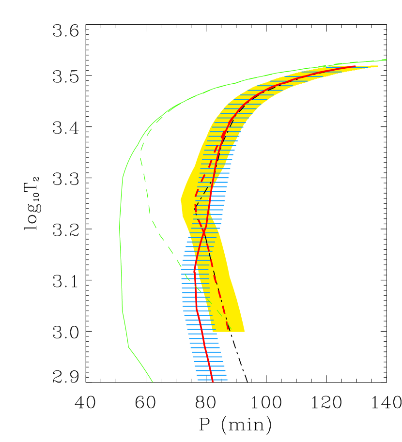
Figure 3: Dependence of the effective temperature $T_{2}$ of a donor on the orbital period $P$. The thick dashed and solid lines plot the semi-empirical $P$–$T_{2}$ relations for the B1 and B5 sequences, respectively, with the dashed and hatched regions denoting the corresponding uncertainties. The thin dashed and solid lines give the unperturbed $P_{0}$–$T_{2,0}$ relations for the B1 and B5 sequences, respectively. The semi-empirical $P$–$T_{2}$ relation of Knigge (2006) is plotted as the dot-dashed line.

2.4 Luminosities and Timescales

Combining equation (12) with the Stefan-Boltzmann law

$$L_{2}=4\pi\sigma R_{2}^{2}T_{2}^{4},$$ (13)

where $\sigma$ is Stefan-Boltzmann constant, one can show that the change in the stellar luminosity is given by

$$L_{2}/L_{2,0}=\alpha^{\frac{22a+4b+6}{5a+2b+5}}.$$ (14)

Although the effective temperature does not change much with the bloating factor, the additional $\alpha^{2}$ term in the Stefan-Boltzmann law increases $L_{2}/L_{2,0}$ significantly. Columns (5) and (10) in Table 1 give the values of $L_{2}$ for the B1 and B5 sequences, respectively.

The nuclear luminosity ${L_{\rm nuc}}$ is determined by the energy produced in the central parts of a donor, so that ${L_{\rm nuc}}\simeq M_{2}\epsilon_{c}$, where $\epsilon_{c}$ is the thermonuclear reaction rate given by

$$\epsilon_{c}\propto T_{c}^{\nu}\rho_{c}^{\eta-1},$$ (15)

with $T_{c}$ and $\rho_{c}$ denoting the central temperature and density, respectively. Since $T_{c}\propto K\rho_{c}^{2/3}\propto\alpha^{-1}$ for a monatomic ideal gas, the change in the nuclear luminosity due to the bloating factor is

$$\frac{{L_{\rm nuc}}}{{L_{\rm nuc,0}}}=\alpha^{3-3\eta-\nu}.$$ (16)

Theoretical models for stellar structure and evolution give $\nu\approx 6$ and $\eta\approx 2$ (Burrows & Leibert, 1993) for $T_{c}\simeq 3\times 10^{6}$ K and $\rho_{c}\simeq 150$ g cm^-3, typical for the centers of low-mass stars.

Since $L_{2,0}={L_{\rm nuc,0}}$ for isolated stars in thermal equilibrium, the gravothermal luminosity satisfies

$$\frac{{L_{\rm g}}}{L_{2}}=1-\frac{{L_{\rm nuc}}}{{L_{\rm nuc,0}}}\frac{L_{2,0}}{L_{2}}.$$ (17)

Thermonuclear burning stops in CV secondaries once they reach the MHBM $\approx{0.075\rm\;M_{\odot}}$. At this point, donors are effectively born as brown dwarfs and the gravitational collapse becomes the dominant source of the stellar radiation. That is, ${{L_{\rm g}}}/{L_{2}}=1$ for $M_{2}\leq{0.075\rm\;M_{\odot}}$.

Figure 4 plots ${{L_{\rm g}}}/{L_{2}}$ versus $M_{2}$ for the B1 and B5 sequences as dashed and solid lines, respectively, with the uncertainties denoted by the shaded and hatched regions. Figures 2 and 4 together imply that at any given mass the contribution of the gravothermal luminosity increases with the bloating factor. If $R_{2}$ increases by $20\%$, more than $80\%$ of the donor luminosity is generated by the release of thermal and gravitational energies.

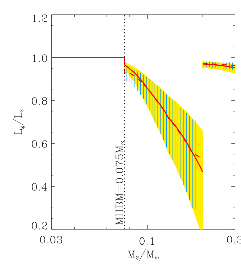
Figure 4: Semi-empirical ratio of the gravothermal luminosity ${L_{\rm g}}$ to the surface luminosity $L_{2}$ as a function of the donor mass. The dashed and solid lines correspond to the B1 and B5 sequences, respectively, with the shaded and hatched regions denoting the uncertainties. For donors below the MHBM, all radiated energy comes from gravothermal collapse (${L_{\rm g}}/L_{2}=1$).

3 Mass-loss Rate

Finding the theoretical mass-loss rates of CV donors is a daunting task since it involves many complicated processes including thermal and adiabatic relaxations, nuclear evolution, effects of tidal and rotational distortions, orbital angular momentum loss, etc., all of which may affect the internal structure significantly. Although the stationary model of Ritter (1988) has been used in various theoretical models of CV evolution, it relies on the parameters describing the donor atmosphere in the vicinity of the inner Lagrangian point, which are poorly known. By relating the mass-loss rate with angular momentum loss, on the other hand, the Ritter model allows to check whether a proposed angular momentum loss mechanism is indeed responsible for CV evolution. As mentioned in §1, the numerical calculations that incorporate the stellar evolution and the mass-loss model of Ritter (1988) produced MRRs that differ from the empirical MRR.

3.1 Semi-empirical Mass-loss Rate

Instead of employing the Ritter model to calculate the mass-loss rate, we seek the ${\dot{M}_{2}}$ that is required to reproduce the empirical MRR. We make use of the well-known relation between the effective mass-radius exponent ${\xi_{\rm E}}$ of the donor and the mass-loss timescale:

$${\xi_{\rm E}}={\xi_{\rm S}}+\tau\frac{7}{3}\frac{{L_{\rm g}}}{L_{2}},$$ (18)

(Ritter, 1996), where ${\xi_{\rm S}}\approx-1/3$ is the adiabatic mass-radius exponent for fully convective stars. Equation (18) dictates how the MRR should behave in response to the mass-loss and thermal relaxation processes. When the mass transfer just commences, ${L_{\rm g}}\approx 0$ and the donor response is adiabatic, leading to ${\xi_{\rm E}}\approx{\xi_{\rm S}}$. Since the ensuing deviation from the adiabatic evolution depends on how the donor reacts thermally on the mass loss, ${\xi_{\rm E}}$ increases linearly with $\tau$ (Ritter, 1996). Combining equations (9), (13) and (18) with the definitions of the Kelvin-Helmholtz timescale (${\tau_{\rm KH}}\equiv GM_{2}^{2}/(R_{2}L_{2}$)) and mass-loss timescale (${\tau_{\rm M}}\equiv M_{2}/\mid{\dot{M}_{2}}\mid$), one obtains

$$-{\dot{M}_{2}}=\frac{1}{({\xi_{\rm E}}+1/3)}\frac{56}{243}\frac{\sigma}{\pi}\frac{{L_{\rm g}}}{L_{2}}T_{2}^{4}P^{2}.$$ (19)

When ${\xi_{\rm E}}=1/3$ corresponding to the period bounce, equation (19) recovers equation (34) of Rappaport et al. (1982) for the mass-loss rate at the minimum period.

In Figure 5 we plot the semi-empirical $P$–${\dot{M}_{2}}$ relations calculated from (19) for the 1-Gyr and 5-Gyr isochrones as dashed and solid lines in red color, respectively. The corresponding uncertainties are given by the shaded and hatched regions. Columns (7) and (12) of Table 1 list the values of ${\dot{M}_{2}}$. The semi-empirical mass-loss rate is essentially non-stationary. For $129$ min $>P>90$ min, ${\dot{M}_{2}}$ is in the range of $\sim 10^{-9.5}$ – $10^{-10}{\rm\;M_{\odot}\;\rm yr^{-1}}$ and decreases relatively slowly as ${\dot{M}_{2}}\propto P^{3}$. Below 90 minutes, ${\dot{M}_{2}}$ sharply declines towards ${P_{\rm min}}$ as a result of a strong dependence of ${\dot{M}_{2}}$ upon $T_{2}$, emulating the $P$–$T_{2}$ relation shown in Figure 3. Since the accretion rate decreases with ${\dot{M}_{2}}$, this rapid decline of ${\dot{M}_{2}}$ is consistent with the observed low accretion activities of CVs within the period spike identified in the SDSS samples (Gånsicke et al., 2009). Note that the mass-loss rates for the B1 and B5 sequence are almost similar to each other for masses above the MHBM, suggesting that these are perhaps permanent values. In the brown dwarf regime, on the other hand, the ambiguity in the adopted stellar age leads to a large difference in the mass-loss rate, suggesting that it is necessary to use the appropriate isochrones for an accurate estimation of ${\dot{M}_{2}}$ for donors with $M_{2}<{0.075\rm\;M_{\odot}}$.

For comparison, Figure 5 also plots as a dot-dashed line the $P$–${\dot{M}_{2}}$ relation from the numerical models of Kolb & Baraffe (1999), which shows a pronounced “boomerang” shape such that ${\dot{M}_{2}}$ is nearly stationary above ${P_{\rm turn}}$ with ${\dot{M}_{2}}\propto P^{0.5}$. It also has ${\dot{M}_{2}}$ significantly smaller for $M_{2}>{0.075\rm\;M_{\odot}}$ than our semi-empirical results. To see what causes the difference between our semi-empirical $P$–${\dot{M}_{2}}$ relation and the numerical result of Kolb & Baraffe (1999), we calculate ${\dot{M}_{2}}$ from equation (19) by using the MRR of Kolb & Baraffe (1999) together with the 5-Gyr isochrone. The resulting $P$–${\dot{M}_{2}}$ relation is plotted in Figure 5 as a dotted line, which is overall in good agreement with the numerical results of Kolb & Baraffe (1999). This suggests that smaller radii of donors in their work are a primary reason for the discrepancies between the results of the current work and Kolb & Baraffe (1999). This also proves to some extent that our approach provides a reasonable way to estimate the mass-loss rate.

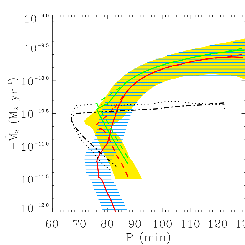
Figure 5: Dependence of the mass-loss rate ${\dot{M}_{2}}$ of a donor on the orbital period $P$. The dashed and solid lines in red give ${\dot{M}_{2}}$ for the B1 and B5 sequences, respectively, with the dashed and hatched regions denoting the uncertainties. The dot-dashed line represents the numerical result of Kolb & Baraffe (1999), while the dotted line plots the mass-loss rate obtained from equation (19) with the numerical MRR of Kolb & Baraffe (1999) for evolving donors. The dashed and solid lines in green denote ${\dot{M}_{2,\rm{R}}}$, for the B1 and B5 sequences, respectively, from the stationary mass-transfer model of Ritter (1988) when the angular momentum loss is dominated by gravitational wave emission.

From the semi-empirical ${\dot{M}_{2}}$, we calculate $\tau$ for the B1 and B5 sequences, which are listed in Columns (8) and (13) of Table 1, respectively. Note that donors in CVs below ${P_{\rm gap}^{~{}-}}$ are out of thermal equilibrium with $\tau\lesssim 1$, which is the main cause of the donor expansion. Equations (17) and (19) imply that for given $M_{2}$ and ${\xi_{\rm E}}$, the mass-loss rate increases more than $\alpha^{3}$ due mainly to changes in the orbital period and gravothermal luminosity. The resulting semi-empirical $P$–${\dot{M}_{2}}$ relation still has a boomerang shape, which is much less dramatic than that of Kolb & Baraffe (1999) due to the donor bloating and the associated thermal relaxation. Nevertheless, it is very difficult to detect the boomerang shape observationally because of the sharp decline of $T_{2}$ and ${\dot{M}_{2}}$ below 90 min.

Once the $P$–$M_{2}$ and $P$–${\dot{M}_{2}}$ relations are found, it is straightforward to calculate the temporal change of the donor mass by solving $dM_{2}/dt={\dot{M}_{2}}$. We assume that donors are 1 Gyr old and have a fixed initial mass of $0.2{\rm\;M_{\odot}}$ when they emerge from the period gap. Since CVs with $P<2$ h are predominantly DNe (Ritter & Kolb, 2003), we further assume that the masses of WDs are constant at $M_{1}=0.75{\rm\;M_{\odot}}$ throughout CV evolution. Figure 6 plots as dashed and solid lines the evolution of donor mass and orbital period calculated from the semi-empirical ${\dot{M}_{2}}$ for the B1 and B5 sequences, respectively, as functions of time $t$ elapsed since ${P_{\rm gap}^{~{}-}}$ (i.e., $t_{0}=1$ Gyr). The dot-dashed lines show $M_{2}(t)$ and $P(t)$ from the mass-loss rate of Kolb & Baraffe (1999) for which $M_{1}=0.6{\rm\;M_{\odot}}$ and $M_{2}=0.21{\rm\;M_{\odot}}$ initially at ${P_{\rm gap}^{~{}-}}$. The changes in the donor mass and orbital period in the numerical model of Kolb & Baraffe (1999) are in general slower because of a lower mass-loss rate. Our semi-empirical results indicate that $M_{2}$ decreases from $0.2{\rm\;M_{\odot}}$ to ${0.075\rm\;M_{\odot}}$ in $\sim 1$ Gyr and that the minimum period is reached in $\sim 1$–$2$ Gyr after ${P_{\rm gap}^{~{}-}}$, without no essential dependence on the adopted stellar age. On the other hand, the numerical model of Kolb & Baraffe (1999) predicts that the same decrement of $M_{2}$ occurs in $\sim 3.5$ Gyr, while it takes the donors $\sim 4$ Gyr to reach ${P_{\rm min}}$. Although uncertainties in the stellar ages make it difficult to follow $M_{2}(t)$ and $P(t)$ accurately below the MHBM, the close agreement between the results based on the B1 and B5 sequences suggests that the ages of CV secondaries with ${0.075\rm\;M_{\odot}}<M_{2}<0.2{\rm\;M_{\odot}}$ are less than 2 Gyr.

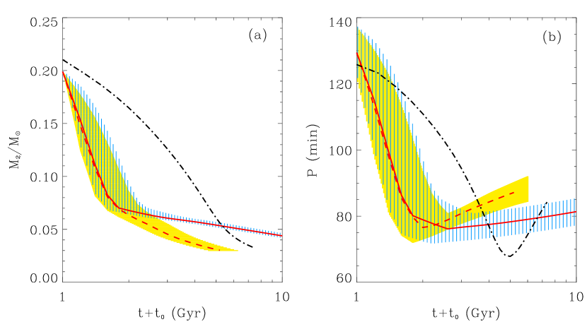
Figure 6: Temporal evolution of (a) the donor mass $M_{2}$ and (b) the orbital period $P$ due to mass loss. Note that $t$ denotes the time measured from the lower bound ${P_{\rm gap}^{~{}-}}$ of the period gap where the donor has an age of $t_{0}=1$ Gyr. The dashed and solid lines are for the B1 and B5 sequences, respectively, with the shaded and hatched regions denoting the uncertaities. The dot-dashed lines show the results from the mass-loss rate of Kolb & Baraffe (1999).

3.2 Consistency check

Mass transfer in CVs below the period gap is considered to be driven by gravitational wave radiation (Paczynski, 1981; Patterson, 1984; Kolb & Baraffe, 1999; Howell et al., 2001). While equation (19) is useful to obtain ${\dot{M}_{2}}$ from the empirical MRR independent of specifics of mass transfer, it does not provide any clue regarding what drives mass transfer in CVs. In this subsection, we make use of the stationary mass-transfer model of Ritter (1988) and check whether the semi-empirical ${\dot{M}_{2}}$ calculated in §3.1 is consistent with the angular momentum loss via emission of gravitational waves.

Ritter (1988) presented a simple analytical model in which the mass transfer from a donor is treated as a stationary isothermal, subsonic flow of gas through the inner Lagrangian point. Taking allowance for the finite scale height of the donor photosphere and considering the temporal changes in the volume radii of the donor and the Roche lobe, Ritter (1988) showed that the stationary mass-transfer rate is given by

$$-{\dot{M}_{2,\rm{R}}}=\frac{M_{2}}{({\xi_{\rm S}}-{\xi_{\rm R}})}\biggl{[}\frac{7}{3}\frac{{L_{\rm g}}}{L_{2}}\frac{1}{{\tau_{\rm KH}}}-\frac{2}{{\tau_{\rm\rm J}}}\biggr{]},$$ (20)

where ${\tau_{\rm\rm J}}$ is the angular momentum loss timescale, ${\xi_{\rm R}}$ is the mass-radius exponent of the critical Roche lobe. Note that we neglect the nuclear-timescale term in equation (20) since it is much longer than the other timescales involved. In the case of DNe for which the mass transfer is non-conservative, ${\xi_{\rm R}}$ is given by

$${\xi_{\rm R}}=-\frac{5}{3}+\biggl{(}\frac{2}{3}+2q\biggr{)}\frac{q}{1+q},$$ (21)

(Soberman et al., 1997). If the gravitational wave emission is the dominant mechanism for the shrinkage of the orbital radius, ${\tau_{\rm\rm J}}$ can be set equal to ${\tau_{\rm\rm G}}$ defined as

$${\tau_{\rm\rm G}}=-\frac{5}{32}\frac{c^{5}}{G^{5/3}}\biggl{(}\frac{P}{2\pi}\biggr{)}^{8/3}\frac{(M_{1}+M_{2})^{1/3}}{M_{1}M_{2}},$$ (22)

(Landau & Lifshitz, 1975).

We use the empirical MRR of Knigge (2006) and solve equation (20) with ${\tau_{\rm\rm J}}={\tau_{\rm\rm G}}$ for ${\dot{M}_{2,\rm{R}}}$. The resulting $P$–${\dot{M}_{2,\rm{R}}}$ relations are plotted in Figure 5 as dashed and solid lines in green color for the B1 and B5 sequences. respectively. The adopted stellar ages make a small difference in ${\dot{M}_{2,\rm{R}}}$, since the first term in the square brackets of equation (20) is insensitive to the isochrones when $M_{2}>$ MHBM, while it becomes much smaller than the second term when $M_{2}<$ MHBM. Figure 5 shows that ${\dot{M}_{2,\rm{R}}}$ agrees, within errorbars, with ${\dot{M}_{2}}$ for both B1 and B5 sequences before reaching the minimum period. This verifies that our semi-empirical mass-loss rate is consistent with the angular momentum loss due to emission of gravitational waves, at least for pre-bouncers. Beyond ${P_{\rm min}}$, ${\dot{M}_{2}}$ for the B1 sequence appears to match ${\dot{M}_{2,\rm{R}}}$ better than the B5 sequence, suggesting that the CV ages are presumably less than 5 Gyr.

4 Discussion

Since the mass-loss rate cannot be observed directly, we are only able to compare our semi-empirical results with the accretion rates estimated by means of other indicators. For this purpose, we select 10 short-period, eclipsing CVs from Patterson et al. (2005), Littlefair et al. (2008), and Townsley & Gånsicke (2009). Table 2 represents a compilation of our sample CVs, with the parameters in Columns (2) to (7) taken from the referred papers. To our knowledge, these are the only eclipsers with $P$ below 130 min, for which the reliable data for the binary parameters such as $P$, $M_{1}$, $M_{2}$, and $T_{1}$ are all available. To infer the mass-accretion rates for the sample CVs, we use

$$T_{1}=1.7\times 10^{4}K\biggl{(}\frac{{\langle\dot{M}_{1}\rangle}}{10^{-10}{\rm\;M_{\odot}\;\rm yr^{-1}}}\biggr{)}^{1/4}\left(\frac{M_{1}}{0.9{\rm\;M_{\odot}}}\right),$$ (23)

where $T_{1}$ and $M_{1}$ are the effective temperature and mass of a WD and ${\langle\dot{M}_{1}\rangle}$ is the time-averaged accretion rate, taken from Townsley & Gånsicke (2009). Since the gravitational energy released by the accreted material onto the surface of a WD is deposited at shallow depths and soon radiated away, the quiescent surface luminosity should be proportional to the mass-accretion rate, leading to $T_{1}\propto{\langle\dot{M}_{1}\rangle}^{1/4}$ (e.g., Townsley & Bildsten 2003, 2004). Filled circles with errorbars in Figure 7a plot ${\langle\dot{M}_{1}\rangle}$ for the sample CVs calculated from equation (23); these are also listed in Column (8) of Table 2. It can be seen that ${\langle\dot{M}_{1}\rangle}$ is broadly in line with our semi-empirical ${\dot{M}_{2}}$ for both B1 and B5 sequence. This suggests that our semi-empirical $P$–${\dot{M}_{2}}$ relation is realistic, provided that $-{\dot{M}_{2}}={\langle\dot{M}_{1}\rangle}$ in these CVs during accretion disk quiescence. Townsley & Gånsicke (2009) noted that ${\langle\dot{M}_{1}\rangle}$ significantly declines towards ${P_{\rm min}}$ for $P<84$ min. Since the accretion rate decreases with decreasing ${\dot{M}_{2}}$, this downward tendency of ${\langle\dot{M}_{1}\rangle}$ with $P$ is in agreement with the behavior of the semi-empirical ${\dot{M}_{2}}$.

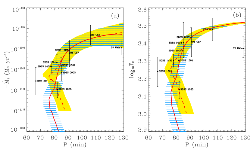
Figure 7: Comparison between our semi-analytic results (lines) and the 10 observed eclipsing CVs (filled circles) listed in Table 2 for (a) the mass-loss rate and (b) the effective temperature. The dashed and solid lines are for the B1 and B5 sequences, respectively, with the shaded and hatched regions denoting the uncertaities. In (b), $T_{2}$ is estimated from equation (24) assuming that mass is conserved (i.e., $-{\dot{M}_{2}}={\langle\dot{M}_{1}\rangle}$).

Donors in short-period CVs are very faint objects, making it difficult to measure their effective temperatures $T_{2}$ directly from observations, especially in the brown dwarfs regime: in our sample, only two systems (HT Cas and DV UMa) have measured $T_{2}$ available in the Ritter & Kolb (2003) catalogue. One way to estimate $T_{2}$ is to use the strong dependence of ${\dot{M}_{2}}$ on $T_{2}$. Assuming that $-{\dot{M}_{2}}={\langle\dot{M}_{1}\rangle}$ during the quiescence phase of DNe, we combine equations (19) and (23) to derive

$$\frac{T_{2}}{T_{1}}\approx 11.594\frac{({\xi_{\rm E}}+1/3)^{1/4}}{P^{1/2}}\biggl{(}\frac{{L_{\rm g}}}{L_{2}}\biggr{)}^{-1/4}\biggl{(}\frac{M_{1}}{0.9{\rm\;M_{\odot}}}\biggr{)}^{-1}.$$ (24)

Since donors with mass below the MHBM have ${L_{\rm g}}/L_{2}=1$, ${T_{2}}/{T_{1}}$ depends only on the orbital period and the effective mass-radius exponent. For masses above the MHBM, on the other hand, an accurate estimation of $T_{2}$ requires to consider the effect of $({L_{\rm g}}/L_{2})^{-1/4}$ term, which can not be determined observationally.

Using the method described in §2.4, we calculate ${L_{\rm g}}/L_{2}$ for the sample CVs listed in Table 2. For this, we take ${\xi_{\rm E}}=0.21\pm 0.1$ for systems with $M_{2}<0.063{\rm\;M_{\odot}}$ and ${\xi_{\rm E}}=0.64\pm 0.02$ for $M_{2}>0.063{\rm\;M_{\odot}}$ in accordance with the adopted empirical MRR. The bloating factor of each system is calculated relative to the 1-Gyr isochrone. We then calculate $T_{2}$ from equation (24) and plot the results in Figure 7b as filled circles with errorbars; these are also tabulated in Column (9) in Table 2. It is remarkable that the estimated effective temperatures, except for SDSS 1507 and DV UMa, are very close to the semi-empirical $P$–$T_{2}$ relation, suggesting that equation (24) is in fact a good way to estimate $T_{2}$ when it cannot be measured observationally. A small orbital period of SDSS 1507 implies that this system is most likely formed directly from a WD/brown dwarf pair (Littlefair et al., 2007) or a member of the old halo (Patterson et al., 2008), rather than a conventional DN. In the case of DV UMa, $T_{2}\approx 2400$ K calculated from equation (24) is $\sim 30\%$ smaller than the observed effective temperature $T_{2}\approx 3200\pm 100$ K, corresponding to a spectral type of M4.5$\pm 0.5$, from the Ritter & Kolb (2003) catalogue. Such a big difference in $T_{2}$ cannot be due to ambiguity in $({\xi_{\rm E}}+1/3)^{1/4}$ or $({L_{\rm g}}/L_{2})^{-1/4}$ terms since both are close to unity for this object. Townsley & Bildsten (2003) noted that the best-constrained quantity from a measured $T_{1}$ is the accretion rate per unit area, $\langle\dot{m}_{1}\rangle=\langle\dot{M_{1}}\rangle/4\pi R_{1}^{2}$, while the subsequent estimation of ${\langle\dot{M}_{1}\rangle}$ from $\langle\dot{m}_{1}\rangle$ requires a certain MRR of WDs, which is poorly known for CVs. The WD mass in DV UMa is highest among the sample, and it is highly probable that the MRR for massive WDs differs from $R_{1}\ \propto M_{1}^{-1.8}$ adopted by Townsley & Gånsicke (2009).

Based on the donor masses, Littlefair et al. (2008) claimed that SDSS 1035, SDSS 1501, SDSS 1507, and SDSS 1433 possess post-period minimum CVs. Although period bouncers should have low $M_{2}$, the precise mass of a particular secondary does not signify its evolutionary history or status (Patterson, 2009). The evolutionary status of such objects can be clarified more clearly by their positions, for instance, on the $P$–$T_{2}$ or $P$–${\dot{M}_{2}}$ diagram where the boomerang effect can be seen. Figure 7 suggests that SDSS 1501 and SDSS 1433 among the sample of Littlefair et al. (2008) have not reached ${P_{\rm min}}$ yet. This result does not depend on the stellar age, since these have $-{\dot{M}_{2}}>10^{-10.5}{\rm\;M_{\odot}\;\rm yr^{-1}}$ for which the semi-empirical mass-loss rate is insensitive to the adopted isochrone. While the evolutionary status of SDSS 1035 is unclear, the fact that the $P$–${\dot{M}_{2}}$ dependence for the B1 sequence reconciles well with that due to gravitational wave emission indicates that it is likely a post-bounce CV.

Kolb & Baraffe (1999) argued that the tidal and the rotational distortions do not change the value of ${P_{\rm turn}}$ appreciably because the internal structure of CV secondaries is only weakly affected by such perturbations. To show this, they compared the effective temperatures of the distorted and undistorted stars and found almost no change in $T_{2}$. This result is totally expected since short-period CVs are fully convective stars. As we showed in §2.3, the Hayashi theory gives that the reaction of $T_{2}$ on the bloating of a donor is small for isolated, fully convective stars. We also show in Appendix B that the influence of an isentropic expansion on $T_{2}$ caused by tidal and rotational distortions can be neglected in most practical cases. All of these suggest that the effective temperature does not reliably measure the amount of the stellar bloating, and consequently can not be used as an indicator of the degree of tidal and rotational distortions.

5 Summary

The mass-loss rate of donors is one of the most important parameters that govern the evolution of short-period CVs. Since the mass-loss rate is not directly observable, most previous work employed either purely numerical methods or semi-empirical approaches that use the observed properties of CV accretors rather than donors. Yet, the confirmation of the resulting mass-loss rates has to be made. In this work, we use the empirical MRR of short-period CVs constructed by Knigge (2006) as an input parameter and derive the semi-empirical relationship between the orbital period and mass-loss rate. We assume that the bloating of CV donors is caused mainly by the mass loss and associated thermal relaxation processes. We also calculate the responses of the effective temperature and luminosities on the bloating of the CV secondaries. We discuss our semi-empirical mass-loss rate in comparison with those from the previous numerical and semi-empirical studies, and in terms of estimating the effective temperature of the donors. Our main results are summarized as follows.

1. The semi-empirical $P$–${\dot{M}_{2}}$ dependence shows that the mass-loss rate is essentially non-stationary. For $P>90$ min, ${\dot{M}_{2}}$ is in the range of $10^{-9.5}$–$10^{-10}{\rm\;M_{\odot}\;\rm yr^{-1}}$ and decreases with decreasing $P$ relatively slowly as ${\dot{M}_{2}}\propto P^{3}$. Below 90 minutes, on the other hand, ${\dot{M}_{2}}$ sharply declines towards ${P_{\rm min}}$ as a result of a strong dependence of ${\dot{M}_{2}}$ upon $T_{2}$, emulating the $P$–$T_{2}$ relation. The $P$-dependence and amplitudes of the semi-empirical ${\dot{M}_{2}}$ are significantly different from those predicted by the purely numerical models of Kolb & Baraffe (1999). The main reason for the discrepancies is small donor radii in the latter. Donors in short-period CVs are out of thermal equilibrium with $\tau\lesssim 1$. Thermal relaxation processes change the slope of the $P$–${\dot{M}_{2}}$ and $P$–$T_{2}$ diagrams significantly above ${P_{\rm min}}$, making the boomerang shape less pronounced. Due to the sharp decline of $T_{2}$ and ${\dot{M}_{2}}$ below 90 min, the observational detection of the boomerang shape on the $P$–${\dot{M}_{2}}$ and $P$–$T_{2}$ is highly unlikely.

2. The semi-empirical $P$–${\dot{M}_{2}}$ relation on the basis of the 1-Gyr isochrone is consistent with that estimated from the mass-transfer model of Ritter (1988) with the angular momentum carried dominantly by gravitational waves. Our semi-empirical $P$–${\dot{M}_{2}}$ relation predicts that after emerging from the period gap, donors lose mass from $0.2{\rm\;M_{\odot}}$ to ${0.075\rm\;M_{\odot}}$ in $\sim 1$ Gyr, and reach the minimum period in $\sim 1$–2 Gyrs, suggesting that the ages of CV secondaries with ${0.075\rm\;M_{\odot}}<M<0.2{\rm\;M_{\odot}}$ are less than 2 Gyrs.

3. For 10 selected eclipsing CVs (listed in Table 2) for which the reliable observational data are available, the accretion rates inferred from the observed effective temperatures of WDs are in good agreement with our semi-analytic mass-loss rates, indicating that our semi-empirical $P$–${\dot{M}_{2}}$ relation is realistic. This also suggests that the effective temperature of a CV secondary can be estimated from the effective temperature of its WD primary through equation (24). When analyzed on the $P$–${\dot{M}_{2}}$ or $P$–$T_{2}$ plane, two CVs (SDSS 1501 and SDSS 1433) that were previously considered as post-bouncers by Littlefair et al. (2008) are most likely to be systems before reaching the minimum period.

Appendix A Isentropic Expansion/Contraction of Polytropic Donors

Even without considering the effect of mass loss, Sirotkin & Kim (2009) showed that the tidal and rotational distortions alone make donors in CVs larger by about $\sim 4$–$8\%$ for $n=1.5$ polytropes and $\sim 2$–$3\%$ for $n=3.5$ polytropes, depending on the mass ratio. In this Appendix, we evaluate the enlargement factor for polytropes with arbitrary $0<n<5$.

Consider a polytropic star with index $n$, mass $M_{2}$, and pressure constant $K$. Its radius is $R_{2,0}$ in isolation. The MRR of the unperturbed polytropes is given by

$$K=N_{n,0}GM_{2}^{(n-1)/n}R_{2,0}^{(3-n)/n},$$ (A1)

where $N_{n,0}$ is the dimensionless pressure constant that varies weakly with $n$ (Chandrasekhar, 1933a). When it is situated in a CV, the presence of tidal and rotational perturbations causes it to expand or contract, depending on $n$, by adjusting the internal structure to restore hydrostatic equilibrium. Let the new equilibrium be achieved at the volume radius $R_{2}$ with the corresponding dimensionless pressure constant $N_{n}$. Since the global internal adjustment occurs in the dynamical timescale, shorter than the thermal timescale and the mass-loss time scale, one may assume that the specific entropy of the gas inside the donor does not change much under the influence of the distortional perturbations.

For isentropic responses (i.e., $K$ is unchanged), the enlargement factor is given simply by

$$\alpha_{\rm isen}\equiv\frac{R_{2}}{R_{2,0}}=\biggl{(}\frac{N_{n}}{N_{n,0}}\biggr{)}^{n/(n-3)}.$$ (A2)

We use a self-consistent field method outlined in Sirotkin & Kim (2009) to construct detailed internal structure of polytropes in hydrostatic equilibrium. We then calculate $N_{n,0}$ and $N_{n}$ for polytropes in critical (i.e., Roche-lobe filling) configurations by varying $n$ and the mass ratio $q=M_{2}/M_{1}$. Figure 8 plots the resulting relative changes, $\Delta R_{2}/R_{2,0}=\alpha_{\rm isen}-1$, in the stellar size as a function of $n$ for $q=0.1$. The behavior of $\alpha_{\rm isen}$ with $M_{2}$ (or with the mass ratio $q$ for $M_{1}=0.75{\rm\;M_{\odot}}$) for $n=3/2$ polytropes is plotted in Figure 2 as a dotted line. Figure 8 shows that $\Delta R_{2}>0$ for $n<3$ or $n\lower 2.0pt\hbox{$\;\buildrel\scriptstyle>\over{\scriptstyle\sim}\;$}3.3$, indicating that the perturbations make the donors bigger; the increase in the equatorial radius is larger than the decrease in the polar radius. On the other hand, critical polytropes with $3<n\lower 2.0pt\hbox{$\;\buildrel\scriptstyle<\over{\scriptstyle\sim}\;$}3.3$ have $\Delta R_{2}<0$, since the perturbations decrease the polar radius much more than increasing the equatorial radius.

Notice a discontinuity at $n=3$ for which one cannot determine the stellar enlargement factor. For these polytropes, the central density is proportional to $R_{2}^{-3}$ and the mass becomes independent of $R_{2}$, making it impossible to constrain the mass from its radius (e.g., Chandrasekhar 1933a). $\Delta R_{2}$ diverges to either positive or negative infinity as $n\rightarrow 3$, indicating that a small change of $n$ near 3 leads to a big difference in $\Delta R_{2}$. This suggests that one should be cautious when treating $n=3$ polytropes numerically. Using SPH simulations, Renvoizé et al. (2002) found that the critical configurations have an enlargement factor $\sim 10$–$12\%$ for $n=3$ polytropes when $q=0.05$–$1.0$. This is presumably due to some (unavoidable) numerical errors in the SPH simulations that somehow change their $n=3$ polytropes to $n\sim 2.7$–$2.8$ ones “effectively”, resulting in $\Delta R_{2}/R_{2,0}=0.10$–$0.12$.

Figure 8: Changes in the volume radius of a polytrope due to the isentropic expansion under tidal and rotational perturbations against the polytropic index $n$, when the mass ratio is $q=0.1$. A binary component expands when $n<3$ or $n\lower 2.0pt\hbox{$\;\buildrel\scriptstyle>\over{\scriptstyle\sim}\;$}3.3$, while it contracts when $3<n\lower 2.0pt\hbox{$\;\buildrel\scriptstyle<\over{\scriptstyle\sim}\;$}3.3$. Note that $n=3$ is a special case where the size of a polytrope cannot be constrained by its mass.

Appendix B Change of Effective Temperature due to Isentropic Expansion

In §2.3, we describe how the effective temperature $T_{2}$ of a fully-convective donor varies due to a homologous expansion using the Hayashi theory. Here we study how $T_{2}$ responds to an isentropic expansion. We assume that the pressure $P_{i}$ in the whole stellar interiors below photosphere depends on temperature as

$$P_{i}=\frac{\Re^{5/2}T^{5/2}}{\mu^{5/2}K^{3/2}},$$ (B1)

where $\mu$ is the mean molecular weight and $\Re$ is the gas constant. The photosphere is determined at the radius where the optical depth is $\tau_{\rm ph}=2/3$. If the radiative pressure is unimportant, the photospheric pressure, $P_{p}$, is given by

$$P_{p}(\tau_{\rm ph})\approx\frac{2}{3}\frac{{\bar{g}}}{\kappa},$$ (B2)

where $\kappa$ is the opacity and ${\bar{g}}=GM_{2}/R_{2}^{2}$ is the mean surface gravity. Using a simple opacity law of the form $\kappa=\kappa_{0}P^{a}_{p}T^{b}$, we obtain

$$P_{p}(\tau_{\rm ph})\approx\biggl{(}\frac{2}{3}\frac{{\bar{g}}}{\kappa_{0}}\frac{1}{T^{b}}\biggr{)}^{\frac{1}{a+1}}.$$ (B3)

Since we assume that the donor is in hydrostatic equilibrium, the photospheric pressure should equal the interior pressure at the interface between the convective interiors and the radiative photospheric layer. Assuming $K=K_{0}$, equations (B1) and (B3) are combined to yield

$$\frac{T_{2}}{T_{2,0}}=\alpha_{\rm isen}^{-\frac{4}{5a+2b+5}}.$$ (B4)

In contrast to the Hayashi theory, the effective temperature decreases due to the donor expansion. Nevertheless, $T_{2}/T_{2,0}=0.99$ for $\alpha_{\rm isen}=1.05$, $a=0.5$, and $b=4.5$, typical values for CV secondaries, so that the change in $T_{2}$ due to the tidal and rotational distortions are still very small and can thus be neglected in practice.

Table 1: The semi-empirical donor sequence for CVs

			1-Gyr						5-Gyr
$M_{2}$	$R_{2}$	$P$	$t+t_{0}$	$\log L_{2}$	$T_{2}$	$\log{\dot{M}_{2}}$	$\tau$		$t+t_{0}$	$\log L_{2}$	$T_{2}$	$\log{\dot{M}_{2}}$	$\tau$
(1)	(2)	(3)	(4)	(5)	(6)	(7)	(8)		(9)	(10)	(11)	(12)	(13)
0.040	0.099	82.769	3.50	-4.625	1273	-11.10	0.24		13.08	-5.513	763	-11.99	0.24
0.044	0.101	81.252	3.10	-4.435	1407	-10.94	0.23		9.74	-5.317	846	-11.83	0.23
0.048	0.103	79.898	2.80	-4.293	1513	-10.83	0.23		7.31	-5.167	914	-11.71	0.23
0.053	0.105	78.676	2.55	-4.194	1588	-10.76	0.23		5.47	-5.011	992	-11.58	0.23
0.057	0.107	77.565	2.33	-4.121	1645	-10.73	0.24		4.08	-4.880	1062	-11.49	0.24
0.063	0.108	76.021	2.05	-3.945	1804	-10.67	0.29		2.64	-4.507	1305	-11.23	0.29
0.065	0.111	77.472	1.95	-3.828	1905	-10.61	0.32		2.30	-4.316	1439	-11.09	0.32
0.069	0.116	79.730	1.80	-3.679	2035	-10.56	0.40		1.87	-4.108	1590	-10.99	0.40
0.075	0.121	82.611	1.70	-3.481	2226	-10.39	0.41		1.72	-3.649	2021	-10.55	0.41
0.078	0.124	84.036	1.65	-3.384	2327	-10.33	0.44		1.67	-3.461	2226	-10.39	0.43
0.082	0.128	86.094	1.59	-3.255	2466	-10.21	0.44		1.60	-3.282	2427	-10.23	0.44
0.086	0.133	88.096	1.56	-3.146	2584	-10.11	0.45		1.57	-3.156	2570	-10.12	0.44
0.090	0.137	90.046	1.53	-3.063	2671	-10.04	0.46		1.54	-3.064	2668	-10.04	0.45
0.095	0.141	91.948	1.50	-2.987	2751	-9.98	0.46		1.52	-2.986	2751	-9.98	0.46
0.099	0.144	93.805	1.47	-2.925	2812	-9.94	0.47		1.49	-2.924	2813	-9.93	0.47
0.103	0.148	95.619	1.44	-2.870	2865	-9.90	0.48		1.46	-2.869	2866	-9.89	0.48
0.107	0.152	97.394	1.41	-2.821	2908	-9.86	0.49		1.43	-2.820	2910	-9.86	0.49
0.111	0.156	99.132	1.38	-2.778	2946	-9.84	0.51		1.40	-2.777	2948	-9.83	0.50
0.116	0.160	100.835	1.36	-2.736	2983	-9.81	0.52		1.38	-2.735	2984	-9.81	0.52
0.120	0.163	102.504	1.34	-2.699	3012	-9.79	0.53		1.36	-2.698	3014	-9.79	0.53
0.124	0.167	104.142	1.32	-2.666	3037	-9.77	0.54		1.34	-2.665	3038	-9.77	0.54
0.128	0.170	105.751	1.30	-2.636	3057	-9.76	0.56		1.32	-2.636	3058	-9.76	0.56
0.132	0.174	107.331	1.28	-2.605	3080	-9.74	0.57		1.30	-2.605	3081	-9.74	0.57
0.137	0.177	108.885	1.26	-2.575	3104	-9.73	0.58		1.28	-2.574	3105	-9.72	0.58
0.141	0.181	110.413	1.24	-2.547	3124	-9.71	0.59		1.26	-2.546	3125	-9.71	0.59
0.145	0.184	111.916	1.22	-2.521	3141	-9.70	0.61		1.24	-2.520	3143	-9.70	0.60
0.149	0.188	113.396	1.20	-2.497	3155	-9.69	0.62		1.22	-2.496	3157	-9.69	0.62
0.154	0.191	114.854	1.18	-2.472	3174	-9.68	0.64		1.20	-2.471	3176	-9.68	0.63
0.158	0.194	116.291	1.16	-2.447	3191	-9.67	0.65		1.18	-2.446	3193	-9.67	0.65
0.162	0.198	117.706	1.15	-2.425	3206	-9.66	0.67		1.16	-2.424	3208	-9.66	0.66
0.166	0.201	119.103	1.13	-2.403	3219	-9.66	0.68		1.15	-2.403	3220	-9.65	0.68
0.170	0.204	120.480	1.11	-2.383	3230	-9.65	0.70		1.13	-2.383	3231	-9.65	0.70
0.175	0.207	121.839	1.10	-2.365	3240	-9.65	0.72		1.11	-2.364	3241	-9.65	0.72
0.179	0.211	123.180	1.08	-2.345	3252	-9.64	0.73		1.09	-2.344	3253	-9.64	0.74
0.183	0.214	124.505	1.06	-2.326	3263	-9.63	0.74		1.07	-2.325	3264	-9.64	0.76
0.187	0.217	125.813	1.05	-2.308	3272	-9.62	0.75		1.05	-2.307	3274	-9.64	0.78
0.191	0.220	127.105	1.03	-2.291	3281	-9.61	0.75		1.03	-2.290	3283	-9.64	0.81
0.196	0.223	128.382	1.01	-2.275	3289	-9.60	0.76		1.02	-2.274	3290	-9.64	0.84
0.200	0.226	129.563	1.00	-2.260	3295	-9.60	0.78		1.00	-2.260	3296	-9.65	0.88

Note. — $M_{2}$ and $R_{2}$ are the mass and radius of the donor in the solar units, respectively; $P$ is the orbital period in minutes; $t$ is the time in Gyr elapsed since the lower bound ${P_{\rm gap}^{~{}-}}$ of the period gap, with $t_{0}=1$ Gyr being the CV age at ${P_{\rm gap}^{~{}-}}$; $T_{2}$ is the effective temperature of the donor in degrees Kelvin; $L_{2}$ is the luminosity of the donor in L_⊙; ${\dot{M}_{2}}$ is the mass-loss rate in units of ${\rm\;M_{\odot}\;\rm yr^{-1}}$; $\tau$ is the dimensionless parameter defined in equation (1).

Table 2: Data on Eclipsing Cataclysmic Variables ($P<130$ min) with estimated effective temperature of WD

System	$P$	$M_{1}$	$q$	$T_{1}$	$M_{2}$	$R_{2}$	${\dot{M}_{1}}$	$T_{2}$	Ref
(1)	(2)	(3)	(4)	(5)	(6)	(7)	(8)	(9)	(10)
SDSS 1507	66.6119	$0.910^{+0.070}_{-0.070}$	$0.0625^{+0.0004}_{-0.0004}$	$11000^{+1250}_{-1250}$	$0.057^{+0.004}_{-0.004}$	$0.097^{+0.003}_{-0.003}$	$-10.78^{+0.33}_{-0.34}$	$1730^{+360}_{-310}$	3
SDSS 1433	78.1066	$0.868^{+0.007}_{-0.007}$	$0.0690^{+0.0030}_{-0.0030}$	$12800^{+950}_{-950}$	$0.060^{+0.003}_{-0.003}$	$0.109^{+0.003}_{-0.003}$	$-10.43^{+0.14}_{-0.15}$	$1990^{+160}_{-160}$	3
SDSS 1501	81.8513	$0.800^{+0.030}_{-0.030}$	$0.0670^{+0.0030}_{-0.0030}$	$12500^{+950}_{-950}$	$0.053^{+0.003}_{-0.003}$	$0.108^{+0.004}_{-0.004}$	$-10.33^{+0.19}_{-0.20}$	$2000^{+240}_{-220}$	3
SDSS 1035	82.0896	$0.940^{+0.010}_{-0.010}$	$0.0550^{+0.0020}_{-0.0020}$	$10100^{+1000}_{-1000}$	$0.052^{+0.002}_{-0.002}$	$0.108^{+0.003}_{-0.003}$	$-10.98^{+0.18}_{-0.20}$	$1370^{+150}_{-150}$	3
SDSS 1502	84.8298	$0.820^{+0.030}_{-0.030}$	$0.1090^{+0.0030}_{-0.0030}$	$12300^{+950}_{-950}$	$0.090^{+0.004}_{-0.004}$	$0.131^{+0.003}_{-0.003}$	$-10.40^{+0.19}_{-0.20}$	$2260^{+300}_{-270}$	3
SDSS 0903	85.0659	$0.960^{+0.030}_{-0.030}$	$0.1170^{+0.0030}_{-0.0030}$	$13000^{+1050}_{-1050}$	$0.112^{+0.004}_{-0.004}$	$0.141^{+0.003}_{-0.003}$	$-10.58^{+0.19}_{-0.20}$	$2470^{+740}_{-430}$	3
SDSS 1227	90.6610	$0.810^{+0.030}_{-0.030}$	$0.1180^{+0.0030}_{-0.0030}$	$15000^{+1250}_{-1250}$	$0.096^{+0.004}_{-0.004}$	$0.140^{+0.003}_{-0.003}$	$-10.03^{+0.20}_{-0.21}$	$2690^{+370}_{-330}$	3
OY Car	90.8928	$0.840^{+0.040}_{-0.040}$	$0.1020^{+0.0030}_{-0.0030}$	$15000^{+2000}_{-2000}$	$0.086^{+0.005}_{-0.005}$	$0.133^{+0.003}_{-0.003}$	$-10.10^{+0.30}_{-0.33}$	$2550^{+500}_{-450}$	1,2,3
HT Cas	106.0560	$0.610^{+0.040}_{-0.040}$	$0.1500^{+0.0100}_{-0.0100}$	$14000^{+1000}_{-1000}$	$0.091^{+0.020}_{-0.020}$	$0.150^{+0.013}_{-0.013}$	$-9.66^{+0.24}_{-0.24}$	$3000^{+470}_{-400}$	1,2
DV UMa	128.2800	$1.041^{+0.024}_{-0.024}$	$0.1510^{+0.0010}_{-0.0010}$	$20000^{+1500}_{-1500}$	$0.157^{+0.010}_{-0.010}$	$0.204^{+0.016}_{-0.016}$	$-9.97^{+0.17}_{-0.18}$	$2380^{+470}_{-300}$	1,2

Note. — $P$ is the orbital period in minutes; $M_{1}$ and $M_{2}$ are the masses of the WD primary and the donor in the solar units, respectively; $q=M_{2}/M_{1}$ is the mass ratio; $T_{1}$ and $T_{2}$ are the effective temperatures of the WD and the donor in degrees Kelvin, respectively; $R_{2}$ is the radius of the donor in the solar units; ${\dot{M}_{2}}$ is the mass-loss rate in units of ${\rm\;M_{\odot}\;\rm yr^{-1}}$; References: (1) Patterson et al. (2005); (2) Townsley & Gånsicke (2009); (3) Littlefair et al. (2008).

References

- Andronov et al. (2003) Andronov, N., Pinsonneault, M., Sills, A. 2003, ApJ, 582, 358A
- Baraffe et al. (1998) Baraffe, I., Chabrier, G., Allard, F., & Hauschildt, P. H. 1998, A&A, 337, 403
- Baraffe et al. (2002) Baraffe, I., Chabrier, G., Allard, F., & Hauschildt, P. H. 2002, A&A, 382, 563
- Baraffe et al. (2003) Baraffe, I., Chabrier, G., Barman, T. S., Allard, F., & Hauschildt, P. H. 2003, A&A, 402, 701
- Barker (2003) Barker, J., & Kolb, U. 2003, MNRAS, 340, 623
- Burrows & Leibert (1993) Burrows, A., & Liebert, J. 1993, RevModPhys, 65, 301
- Chandrasekhar (1933a) Chandrasekhar, S. 1933, MNRAS, 93, 390
- Chandrasekhar (1939) Chandrasekhar, S. 1939, An introduction to the study of stellar structure (Chicago Univ. Press)
- D’Antona et. al. (1989) D’Antona, F., Mazzitelli, I., Ritter, H. 1989, A&A, 225, 391
- Eggleton (1983) Eggleton, P. P. 1983, ApJ, 268, 368
- Hansen & Kavaler (1995) Hansen, C. J., & Kawaler, S., D. 1995, Stellar interiors Physical principles, Structure, and Evolution, ed. Appenzeller, I., Harvit, M., Kippenhahn, R., Strittmatter, P., A., (Springel-Verlag, New-York, Inc.)
- Howell et al. (2001) Howell, S. B., Nelson, L. A., & Rappaport, S. 2001, ApJ, 550, 897
- King (1988) King, A. R. 1988, QJRAS, 29, 1
- Kippenhahn & Weigert (1990) Kippenhahn, R., Trimble, V., & Weigert, A. 1990, Stellar Structure and Evolution, ed. Harvit, M., Kippenhahn, R., Trimble, V., Zahn, J.-P., (Springel-Verlag, Berlin Heidelberg)
- Knigge (2006) Knigge, C. 2006, MNRAS, 373, 484
- Kolb & Baraffe (1999) Kolb, U., & Baraffe, I. 1999, MNRAS, 309, 1034
- Kopal (1972) Kopal, Z. 1972, Adv. Astron. Ap. 9, 1
- Landau & Lifshitz (1975) Landau, L. D., & Lifshitz, E. M. 1975, The Classical Theory of Fields, 4th edn. (Pergamon, New York)
- Littlefair et al. (2008) Littlefair, S. P., Dhillon, V. S., Marsh, T. R., Gänsicke, B. T., Baraffe, I., & Watson, C. A. 2008, MNRAS, 388, 1582
- Littlefair et al. (2007) Littlefair, S. P., Dhillon, V. S., Marsh, T. R., Gänsicke, B. T., Baraffe, I., & Watson, C. A. 2007, MNRAS, 381, 827
- Paczynski (1981) Paczynski, B. 1981, Acta Astron., 31, 1
- Patterson (1984) Patterson, J., et al. 1984, ApJS, 54, 443
- Patterson et al. (2005) Patterson, J., et al. 2005, PASP, 117, 1204
- Patterson (2009) Patterson, J. 2009, MNRAS, submitted (arXiv:0903.1006)
- Patterson et al. (2008) Patterson, J., Thorstensen, J. R., & Knigge, C. 2008, PASP, 120, 510
- Rappaport et al. (1982) Rappaport, S., Joss, P. C., & Webbink, R. F. 1982, ApJ, 254, 616
- Renvoizé et al. (2002) Renvoizé, V., Baraffe, I., Kolb, U., & Ritter, H. 2002, A&A, 389, 485
- Rezzolla et. al. (2001) Rezzolla, L., Uryu, K., & Yoshida, S. 2001, MNRAS, 888
- Ritter (1988) Ritter, H. 1988, A&A, 202,93
- Ritter (1996) Ritter, H. 1996, in Evolutionary Processes in Binary Stars, Proceedings of the NATO Advanced Study Institute, Cambridge, ed. Wijers, R., & Davies, M., 477, 223
- Ritter & Kolb (2003) Ritter, H., & Kolb, U. 2003, A&A, 404, 301
- Sirotkin & Kim (2009) Sirtokin, F. V., & Kim, W.-T. 2009, ApJ, 698, 715(SK09)
- Sion (1995) Sion, E., M., 1995, ApJ, 438, 876
- Soberman et al. (1997) Soberman, G. E., Phinney, E.S., & Heuvel E.P.J. 1997, A&A, 327, 620
- Stehle et al. (1996) Stehle, R., Ritter, H., & Kolb, U. 1996, MNRAS, 279, 581
- Townsley & Bildsten (2003) Townsley D. M., & Bildsten L. 2003, ApJ, 596, L227
- Townsley & Bildsten (2004) Townsley D. M., & Bildsten L. 2004, ApJ, 600, 390
- Townsley & Gånsicke (2009) Townsley, D. M., & Gånsicke, B. T. 2009, ApJ, 693, 1007
- Gånsicke et al. (2009) Gånsicke, B. T. et al. 2009, MNRAS, 397, 2170
- Uryu & Eriguchi (1999) Uryu, K., & Eriguchi, Y. 1999, MNRAS, 303, 329
- Urban & Sion (2006) Urban, J. A, & Sion E. M. 2006, ApJ, 642, 1029