Numerical analysis of relaxation times of multiple quantum coherences in the system with a large number of spins

Abstract

We study the decay of multiple quantum (MQ) NMR coherences in systems with the large number of equivalent spins. As being created on the preparation period of MQ NMR experiment, they decay due to the dipole-dipole interactions (DDI) on the evolution period of this experiment. It is shown that the relaxation time decreases with the increase in MQ coherence order (according to the known results) and in the number of spins. We also consider the modified preparation period of MQ NMR experiment (G.A.Alvarez, D.Suter, PRL 104, 230403 (2010)) concatenating the short evolution periods under the secular DDI Hamiltonian (the perturbation) with the evolution period under the non-secular averaged two-spin/two-quantum Hamiltonian. The influence of the perturbation on the decoherence rate is investigated for the systems consisting of 200-600 equivalent spins.

I Introduction

Multiple quantum (MQ) coherences are quite suitable for investigations of the dependence of the relaxation time on the size of the quantum system KS1 ; KS2 ; AS ; CCCR . This problem is closely connected to the estimations of the decoherence time as an important parameter for the quantum information systems. A simplest model of the quantum register formed by the highly correlated spins can be created in MQ NMR experiments BMGP . Some models of quantum registers consisting of up to 4900 qubits were studied experimentally KS2 . The theoretical methods (for example, ref.FF ) describing the experiments KS1 are phenomenological ones and the development of theoretical and numerical approaches from ”the first principles” are fully justified. At the same time, numerical methods of MQ NMR dynamics allow us, generally speaking, to investigate systems consisting of not more than twenty spins DFGM . Some progress in the study of the larger systems (up to 40 spins) is achieved due to the special techniques based on the Chebyshev polynomial expansion DRKH ; ZCAPCDRV and on the phenomenon of quantum parallelism ADLP . The new perspectives are opened by MQ NMR in systems of equivalent spins where the special method has been worked out DFFZ1 ; DFFZ2 allowing one to investigate MQ NMR dynamics of hundreds of spins and even more. Such systems of equivalent spins can be created in a nanopore compound placed in a strong external magnetic field if the nanopores are filled with a gas of spin-carring molecules (atoms) BKHWW ; FR . Since the characteristic time of the molecular diffusion is much less than the spin flip-flop time BKHWW ; FR , the dipole-dipole interactions (DDI) of spins are averaged ( but not to zero) and the residual DDI can be described by the single coupling constant. As a result, all spins can be considered as equivalent ones, which significantly simplifies the numerical simulations.

The above method can be applied to the investigation of the decay of MQ NMR coherence intensities of different orders caused by the secular DDI in systems containing hundreds of spins. In the simplest case this decay occurs on the evolution period of the MQ NMR experiment KS1 . However, the MQ NMR experiment can be modified, for instance, using a different set of pulses on the preparation period, as in Ref.AS . In the later case, the decay takes place on the preparation period.

In this paper we study the decay of MQ NMR coherence intensities created in systems with a large number of equivalent spins. The paper is organized as follows. The general description of different MQ NMR experiments is given in Sec.II. The theory and the numerical simulation of the decay of MQ NMR coherence intensities in different MQ NMR experiments is developed in Sec.III. The conservation law associated with considered models is derived in Sec.IV. We briefly summarize our results in concluding Sec.V.

II The MQ NMR experiments in a system of equivalent spins

The MQ NMR experiment consists of four distinct periods of time (Fig.1): preparation ($\tau$), evolution ($t$), mixing ($\tau$) and detection.

Figure 1: The basic scheme of the MQ NMR experiment. The Hamiltonian $H_{eff}$ (Eq.(7)), $H_{ev}$ (Eq.(10))and $\bar{H}_{MQ}$ (Eq.(5)) govern the spin dynamics on the appropriate period of the MQ NMR experiment

Preparation period.

The spin system is irradiated by the proper multipulse sequence on the preparation period. As a result, the anisotropic DDI of nuclear spins in the external magnetic field, $\vec{B}$, (directed along the axis $z$) oscillates rapidly. In the rotating reference frame G , the dynamics of spin system is described by the effective Hamiltonian $H_{eff}$. We consider two types of pulse sequences on the preparation period. The first one is the standard pulse sequence resulting in the averaged non-secular two-spin/two-quantum Hamiltonian, describing the MQ NMR dynamics on the preparation period of the standard MQ NMR experiment WSWP ; BMGP , i.e. $H_{eff}\equiv H_{MQ}$:

$$H_{MQ}=H^{(+2)}+H^{(-2)},$$ (1)

$$H^{(\pm 2)}=-\frac{1}{2}\sum_{j<k}D_{jk}I^{\pm}_{j}I^{\pm}_{k},$$ (2)

Here $D_{jk}=\gamma^{2}\hbar(1-3\cos^{2}\theta_{jk})/(2r^{3}_{jk})$ is the coupling constant between spins $j$ and $k$, $\gamma$ is the gyromagnetic ratio, $r_{jk}$ is the distance between spins $j$ and $k$, $\theta_{jk}$ is the angle between the vectors $\vec{r}_{jk}$ and $\vec{B}$ and $I^{\pm}_{j}=I_{jx}\pm iI_{jy}$ are the raising and lowering operators of spin $j$. The second type of pulse sequences is introduced in Ref.AS , where a modification of the preparation period of the MQ NMR experiment was suggested. In this case, the preparation period consists of the cycles of the duration $\tau_{c}$ and each cycle concatenates the short evolution period $\tau_{dz}$ under the perturbation Hamiltonian $H_{dz}$ (which is responsible for the secular DDI G ),

$$H_{dz}=\sum_{j<k}D_{jk}(2I_{jz}I_{kz}-I_{jx}I_{kx}-I_{jy}I_{ky})$$ (3)

with the evolution period $\tau_{MQ}$ under the ideal MQ Hamiltonian $H_{MQ}$ (1). Thus, $\tau_{c}=\tau_{dz}+\tau_{MQ}$. Introducing the relative strength $p=\tau_{dz}/\tau_{c}$ ($0\leq p\leq 1$) of the perturbation one can find that the resulting evolution can be described by the effective Hamiltonian $H_{eff}$ given by the following equation AS :

$$H_{eff}(p)=(1-p)H_{MQ}+pH_{dz}.$$ (4)

Let the preparation period consist of $K$ (a big number) cycles of the duration $\tau_{c}$, so that one can introduce the parameter $\tau=K\tau_{c}$. Note, that $H_{eff}(0)\equiv H_{MQ}$, which means that the standard preparation period, used, for instance, in ref. BMGP , is a particular case of the described modification.

Hereafter we study the MQ NMR dynamics of equivalent spins. Such a case can be realized, for instance, by the dipolar coupling spins in a nanopore where the Hamiltonian (1) is averaged ( but not to zero) by the fast molecular diffusion BKHWW ; FR . The Hamiltonians $H_{MQ}$ and $H_{dz}$ with the averaged coupling constant $D$ ($D\tau_{c}\ll 1$) can be rewritten as follows DFFZ1 ; DFFZ2 :

$$\bar{H}_{MQ}=-\frac{D}{4}\{(I^{+})^{2}+(I^{-})^{2}\},$$ (5)

$$\bar{H}_{dz}=\frac{D}{2}\{3I^{2}_{z}-I^{2}\},$$ (6)

where $I^{\pm}=\sum\limits_{j=1}^{N}I^{\pm}_{j}$ ($N$ is the number of spins), $I_{z}=\sum\limits_{j=1}^{N}I_{zj}$ and the operator $I^{2}$ is the square of the total spin angular momentum. Thus Eq.(4) must be replaced with the following one

$$H_{eff}(p)=(1-p)\bar{H}_{MQ}+p\bar{H}_{dz},$$ (7)

which is valid for the system of equivalent spins.

Evolution period.

Let the spin system be governed by the following general Hamiltonian $H_{ev}$ on the evolution period:

$$H_{ev}=(1-\theta(p))\bar{H}_{dz}+\Delta I_{z},\;\;\theta=\left\{\begin{array}[]{ll}0,&p=0\cr 1,&p>0\end{array}\right..$$ (10)

The offset $\Delta$ encodes MQ NMR coherences of different orders, see below, Eq. (16) and ref.BMGP .

Mixing period.

The spin system on the mixing period is governed by the Hamiltonian $-\bar{H}_{MQ}$ in all experiments considered in this paper.

We emphasize that the decay of MQ NMR coherences is caused by the Hamiltonian $\bar{H}_{dz}$ appearing either on the evolution period (if $p=0$ in Eqs.(7,10)) or on the preparation period (if $p\neq 0$ in eqs.(7,10)). These two cases are considered separately in Secs.III.1 and III.2 respectively.

III The decay of MQ NMR coherence intensities caused by the secular DDI

III.1 The decay of MQ NMR coherences in MQ NMR experiments of Ref. BMGP

We consider the time evolution of the coherences in MQ NMR experiments with the standard preparation period BMGP . For this purpose we take $p=0$ in Eqs.(7) and (10), which read:

$$H_{eff}=\bar{H}_{MQ},\;\;H_{ev}=\bar{H}_{dz}+\Delta I_{z},$$ (11)

so that the coherence decay occurs on the evolution period. In order to investigate the MQ NMR dynamics of the system one should find the density matrix $\rho(\tau)$ on the preparation period solving the Liouville evolution equation G

$$i\frac{d\rho(\tau)}{d\tau}=[\bar{H}_{MQ},\rho(\tau)]$$ (12)

with the initial thermodynamic equilibrium state $\rho(0)=I_{z}$ in the high temperature approximation G . Taking into account the pointed information about the Hamiltonians on the different periods of MQ NMR experiment one can write the expression for the longitudinal polarization $\langle I_{z}\rangle(\tau,t)$ after the mixing period of MQ NMR experiment (Fig.1) as follows:

$$\langle I_{z}\rangle(\tau,t)={\mbox{Tr}}\{U^{+}(\tau)e^{-i\Delta tI_{z}}e^{-i\bar{H}_{dz}t}U(\tau)\times$$ (13)

$$I_{z}U^{+}(\tau)e^{i\Delta tI_{z}}e^{i\bar{H}_{dz}t}U(\tau)I_{z}\}=$$

$${\mbox{Tr}}\{e^{-i\Delta tI_{z}}e^{-i\bar{H}_{dz}t}\rho(\tau)e^{i\bar{H}_{dz}t}e^{i\Delta tI_{z}}\rho(\tau)\},$$

where $\rho(\tau)=U(\tau)I_{z}U^{+}(\tau)$ is the solution to Eq.(12) and $U(\tau)=\exp(-i\bar{H}_{MQ}\tau)$. It is convenient to expand the spin density matrix $\rho(\tau)$ in the series as follows

$$\rho(\tau)=\sum_{k}\rho_{k}(\tau),$$ (14)

where $\rho_{k}(\tau)$ is the contribution to $\rho(\tau)$ from MQ coherence of the $k$th order and satisfies the following commutation relation FL :

$$e^{-i\Delta tI_{z}}\rho_{k}e^{i\Delta tI_{z}}=e^{-ik\Delta t}\rho_{k}.$$ (15)

Then Eq.(13) reads

$$\langle I_{z}\rangle(\tau,t)=\sum_{k}e^{-ik\Delta t}{\mbox{Tr}}\{e^{-i\bar{H}_{dz}t}\rho_{k}(\tau)e^{i\bar{H}_{dz}t}\rho_{-k}(\tau)\}.$$ (16)

Eq.(16) defines the intensity $J_{k}(\tau,t)$ of the MQ NMR coherence of order $k$ as follows:

$$J_{k}(\tau,t)={\mbox{Tr}}\{e^{-i\bar{H}_{dz}t}\rho_{k}(\tau)e^{i\bar{H}_{dz}t}\rho_{-k}(\tau)\}.$$ (17)

In analogy to the autocorrelation function for the decay of the transverse magnetization G , Eq.(17) reveals the decay of MQ NMR coherences due to the secular DDI on the evolution period. Since we consider a system of equivalent spins, numerical simulation of Eq.(17) may be simplified allowing one to perform calculations in the systems with the large number of spins. This happens due to the commutation relation

$$[\bar{H}_{MQ},I^{2}]=0,$$ (18)

which suggests us to use the basis of common eigenvectors of $I^{2}$ and $I_{z}$ DFFZ1 . It was shown DFFZ1 ; DFFZ2 that the Hamiltonians $\bar{H}_{MQ}$, $\bar{H}_{dz}$ and the density matrix $\rho(\tau)$ for the system of equivalent spins have a block structure. For instance, $\bar{H}_{MQ}={\mbox{diag}}\{\bar{H}^{\frac{N}{2}}_{MQ},\bar{H}^{\frac{N}{2}-1}_{MQ},\dots,\bar{H}^{\frac{N}{2}-\left[\frac{N}{2}\right]}_{MQ}\}$, ($[a]$ is an integer part of $a$) . These blocks correspond to different total spin numbers $S=N/2,N/2-1,\dots,N/2-[N/2]$ LL . All blocks are degenerated and their degeneracy $n_{N}(S)$ is determined as follows LL :

$$n_{N}(S)=\frac{N!(2S+1)}{(\frac{N}{2}+S+1)!(\frac{N}{2}-S)!},\;\;0\leq S\leq\frac{N}{2}.$$ (19)

Thus, the problem is reduced to the set of analogous problems of lower dimensions. The intensities of MQ NMR coherences $J_{k,S}(\tau,t)$ can be calculated for all blocks. Then the observable intensities $J_{k}(\tau,t)$ ($-N\leq k\leq N$) are following DFFZ1 :

$$J_{k}(\tau,t)=\sum_{S}n_{N}(S)J_{k,S}(\tau,t).$$ (20)

The results of numerical simulations of these intensities are represented below.

III.1.1 The numerical simulations

We study the dynamics of MQ NMR coherence intensities in the nanopore filled with the spin-carring particles numerically. Let us emphasize one more time that we are dealing with the highly symmetrical model where any two spins interact with the same constant of DDI because the diffusion characteristic time in the nanopore is much shorter then the spin flip-flop time BKHWW ; FR . This fact simplifies the numerical calculations significantly since all particles are ”nearest neighbors” in this model and we consider interactions among all of them.

Our calculations showed DFFZ1 that MQ NMR coherence intensities are quickly oscillating functions. For this reason we follow the strategy of Ref. DFFZ1 and consider the averaged intensities

$$\bar{J}_{k}(\bar{t})=\frac{1}{2T}\int_{\tau_{0}}^{\tau_{0}+2T}J_{k}(\bar{\tau},\bar{t})d\bar{\tau},$$ (21)

$$\tau_{0}=31,\;\;T=2\pi/\lambda_{min}=2\pi/\sqrt{3}.$$

where $\bar{\tau}=D\tau$ and $\bar{t}=Dt$ are the dimensionless times associated with the preparation and evolution periods respectively, $\lambda_{min}$ is the minimal eigenvalue of the $\bar{H}_{MQ}$ Hamiltonian. This value belongs to the block $\bar{H}_{MQ}^{\frac{3}{2}}$ of the Hamiltonian DFFZ1 . The choice of $\tau_{0}$ is motivated by the requirement that the coherences of all possible orders have appeared and one can think that the quasi-stationary distribution of the intensities is realized, which has been verified in ref.DFFZ1 . The averaging is performed over two maximal periods $T$ of oscilations, which is taken from the requirement that the increase of the averaging interval does not change $\bar{J}_{k}$ DFFZ1 ; DFFZ2 . The averaged intensities decay with the time $\bar{t}$ of the evolution period. The time moments $t_{e}$ (such that $\bar{J}_{k}(0)/\bar{J}_{k}(\bar{t})|_{\bar{t}=t_{e}}=e$ for an arbitrary $k$) versus MQ coherence order in systems with 201, 401 and 601 spins are shown in Fig.2. We can see from this figure that

1. MQ NMR coherence decay times decrease with the increase in the number of spins;

2. MQ NMR coherence decay times decrease with the increase in their order.

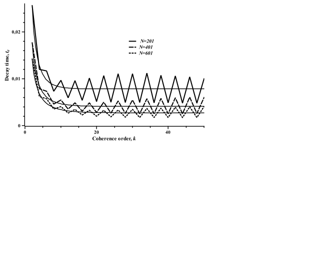
Figure 2: The decay time as a function of the coherence order for the spin systems with $N=201$, 401 and 601.

The times $t_{e}(k)$ of the decay of MQ NMR coherences of order $k>0$ can be approximated by the hyperbolic cotangent, as it is shown in Fig.2:

$$t_{e}(k)=a_{1}\coth(a_{2}k+a_{3}),$$ (22)

where parameters $a_{1},a_{2},a_{3}$ may be found by the least square method:

$$t_{e}(k) = 0.0078\coth(0.1966k-0.0758),\;\;N=201,$$

$$t_{e}(k) = 0.0041\coth(0.1441k-0.0495),\;\;N=401,$$

$$t_{e}(k) = 0.0027\coth(0.1144k-0.0324),\;\;N=601.$$

Figure 3: The evolution of the ”cluster size” $N_{c}$; $\bar{t}$ is the dimensionless evolution time

The approximation given by Eq.(22) shows that the decay rate of the high order coherence intensities is almost independent on their order. This happens because MQ coherence phases (acquired during the evolution period) are approximately proportional to their order, see Eq. (15). As a result, the rates of MQ coherence decays increase with their order and the decay time $t_{e}(k)$ is $\sim 1/k$. Thus, for the high order coherences, we have $t_{e}(k)/t_{e}(k+1)\to 1$, i.e. the decay times of the $k$th and $(k+1)$th coherences are almost the same, which is reflected in Eq.(22). Regarding the zero-order coherence, its intensity $\bar{J}_{0}$ does not decay owing to the commutation relation $[\bar{H}_{dz},\rho_{0}]=0$, which follows from the fact that both $\bar{H}_{dz}$ (6) and $\rho_{0}$ are diagonal in the chosen basis.

It is worthwile to note that the dynamics of the multi-spin cluster growth during the evolution of the solid spin system considered, for instance, in BMGP ; KS3 is essentially different in comparison with that in the system of equivalent spins. The matter is that only the strongly interacting spins are joined in the clusters initially, usually the nearest neighbors in the crystal lattice BMGP ; KS3 . After that, the next neighbors become involved in the cluster and so on. Thus more and more remote spins become embedded in the cluster with time. As a result, it becomes possible to observe the growth of the multi-spin clusters in MQ NMR experiments BMGP ; KS3 . However, the dynamics of the spin clusters is quite different in the high symmetrical spin system such as the system of equivalent spins. All spins are ”nearest neighbors” in this case, so that the spin cluster consisting of all $N$ spins is formed much more quickly during the time interval $\sim 1/D$, where $D$ is the constant of DDI, which is the same for any two spins. It becomes hard to follow the process of the cluster growth in the high symmetrical system of equivalent spins, unlike the solids BMGP ; KS3 . Nevertheless, there is some reorganization of the spin cluster diring the evolution, when the system is irradiated by the multipulse sequence WSWP ; BMGP , resulting to the high order MQ coherences.

Now let us turn to the decay of MQ NMR coherences. We consider the ”cluster” of MQ NMR coherences as a family of such coherences whose intensities exceed some fixed value $J_{min}$, say, $J_{min}=0.005$. This minimal value is taken since the smaller intensities are hardly observable in the experiment. The size $N_{c}$ of the cluster of MQ coherences does evolve, which is demonstrated in Fig.3. This evolution is a consequence of the fact that the rate of the decay increases with the increase in the order of MQ NMR coherences. We see also that the rate of decrease of the coherence cluster size increases with the increase in $N$. The described experiment may be used in order to prepare the coherence clusters of desirable size varying the duration of the evolution period.

III.2 The decay of MQ NMR coherences in MQ NMR experiments with the modified preparation period

It is very important to investigate the degradation of quantum superposition states. MQ NMR experiments BMGP allow us to make it. To this end the modification of the preparation period of the MQ NMR experiment was suggested in ref.AS . In this section we consider Eqs.(7) and (10) with $p>0$, so that the system is governed by the general Hamiltonian $H_{eff}$ during the preparation period and by the Hamiltonian $H_{ev}=\Delta I_{z}$ during the evolution period. Thus the coherence decay occurs on the preparation period of the MQ NMR experiment. The calculations analogous to those used for the derivation of Eq.(17) yield the following expression for the intensities of MQ NMR coherences:

$$J_{k}(\tau,p)={\mbox{Tr}}\{\tilde{\rho}_{k}(\tau,p)\rho_{-k}(\tau,p)\},\;\;\;\tau=K\tau_{c},$$ (23)

where

$$\tilde{\rho}(\tau,p)=e^{-i\tau H_{eff}}I_{z}e^{i\tau H_{eff}}=\sum_{k}\tilde{\rho}_{k}.$$ (24)

If $p\ll 1$, then it is simple to demonstrate that the intensities vary proportionally to $p^{2}$. In fact, the Liouville equation on the preparation period can be rewritten as follows:

$$i\frac{\tilde{\rho}(\tau)}{d\tau}=[(1-p)\bar{H}_{MQ}+p\bar{H}_{dz},\tilde{\rho}(\tau)].$$ (25)

Solving Eq.(25) by the methods of the perturbation theory G one can obtain

$$\tilde{\rho}(\tau)=\rho(\tau)-p\rho_{1}(\tau)-p^{2}\rho_{2}(\tau),$$ (26)

$$\rho_{1}(\tau)=i\int_{0}^{\tau}[e^{i\bar{H}_{MQ}(\tau^{\prime}-\tau)}(\bar{H}_{dz}-$$

$$\bar{H}_{MQ})e^{-i\bar{H}_{MQ}(\tau^{\prime}-\tau)},\rho(\tau)]d\tau^{\prime},$$

$$\rho_{2}(\tau)=\int_{0}^{\tau}d\tau^{\prime}\int_{0}^{\tau^{\prime}}d\tau^{\prime\prime}[e^{i\bar{H}_{MQ}(\tau^{\prime}-\tau)}(\bar{H}_{dz}-$$

$$\bar{H}_{MQ})e^{-i\bar{H}_{MQ}(\tau^{\prime}-\tau)},[e^{i\bar{H}_{MQ}(\tau^{\prime\prime}-\tau)}(\bar{H}_{dz}-$$

$$\bar{H}_{MQ})e^{-i\bar{H}_{MQ}(\tau^{\prime\prime}-\tau)},\rho(\tau)]],$$

where $\rho(\tau)$ is the solution to Eq.(12). It is evident from Eq.(26) that

$${\mbox{Tr}}\{\tilde{\rho}(\tau)\rho(\tau)\}={\mbox{Tr}}\{\rho^{2}(\tau)\}-p^{2}A(\tau),$$ (27)

$$A(\tau)=\int_{0}^{\tau}d\tau^{\prime}\int_{0}^{\tau^{\prime}}d\tau^{\prime\prime}{\mbox{Tr}}\Big{\{}$$

$$[\rho(t),e^{i\bar{H}_{MQ}(\tau^{\prime}-\tau)}(\bar{H}_{dz}-\bar{H}_{MQ})e^{-i\bar{H}_{MQ}(\tau^{\prime}-\tau)}]\times$$

$$[e^{i\bar{H}_{MQ}(\tau^{\prime\prime}-\tau)}(\bar{H}_{dz}-\bar{H}_{MQ})e^{-i\bar{H}_{MQ}(\tau^{\prime\prime}-\tau)},\rho(\tau)]\Big{\}}.$$

The behavior of the intensities with the increase in $p$ is defined by the sign of $A(\tau)$. We do not determine this sign for an arbitrary $\tau$. However, one has for small $\tau$:

$$A\approx-\frac{\tau^{2}}{2}{\mbox{Tr}}[\rho,\bar{H}_{dz}-\bar{H}_{MQ}]^{2}>0.$$ (28)

Since ${\mbox{Tr}}\{\rho^{2}\}$ is the sum of the intensities of MQ NMR coherences for the standard MQ NMR experiment and ${\mbox{Tr}}\{\tilde{\rho}(\tau)\rho(\tau)\}$ is the analogous sum, when the perturbations are taken into account one can conclude that the intensities decrease with the increase in the square of the perturbation strength at least for small $\tau$, which is confirmed below by the numerical simulations.

III.2.1 The numerical simulations

We refer to $\bar{\tau}=D\tau$ as the dimensionless evolution time in this section. Before proceed to the numerical simulations, let us underline the basic difference between the experiments considered in Secs.III.1 and III.2. The matter is that the high frequency oscillations of MQ NMR coherences are formed on the preparation period with the duration $\tau$, while the decay of these coherences occurs on the evolution period (with the duration $t$) in Sec.III.1. For this reason we consider the intensities averaged over the parameter $\tau$ in that section. However, the situation is different in Sec.III.2, because the decay occurs on the preparation period, so that the parameter $\tau$ is responsible for the both oscilations and decay of MQ NMR coherences. Because of this fact, we are not able to consider the averaged intensities.

Instead of this, we relate the decay time $\tau_{p}(k)$ of the intensity $J_{k}(\bar{\tau})$ with the decay times $\tau_{p}^{\pm}(k)$ of its envelopes. Here the subscript $p$ indicates that the parameter $\tau_{p}$ depends on the value of $p$ in the Hamiltonian $H_{eff}$. Parameters $\tau_{p}^{\pm}(k)$ may be found simply by plotting the graphs of the envelopes $\hat{J}_{k}^{\pm}(\bar{\tau})$ of the quickly oscillating intensity $J_{k}(\bar{\tau})$, $\hat{J}_{k}^{-}(\bar{\tau})\leq J_{k}(\bar{\tau})\leq\hat{J}_{k}^{+}(\bar{\tau})$. Then the decay times of the envelopes $\tau_{p}^{\pm}(k)$ are the first zeros of $\hat{J}_{k}^{\pm}(\bar{\tau})$ appeared after the amplitude of the $k$th intensity gets its maximal value: $\hat{J}_{k}^{\pm}(\tau^{env}_{p}(k))=0$. All this suggests us to calculate the decay time $\tau_{p}(k)$ of the $k$th coherence as follows. First, we have to find numerically all solutions $\tau_{p}^{(i)}(k)$ ($i=1,2,\dots$) to the equation $J_{k}(\bar{\tau},p)|_{\bar{\tau}=\tau_{p}^{(i)}(k)}=0$, such that $\tau^{-}_{p}(k)<\tau_{p}^{(i)}(k)\leq\tau^{+}_{p}(k)$. Let $N_{p}(k)$ be the number of such solutions. Then the decay time of the $k$th coherence intensity may be found as the averaged value of these solutions: $\tau_{p}(k)=\frac{1}{N_{p}(k)}\sum_{i=1}^{N_{p}(k)}\tau_{p}^{(i)}(k)$. The dependence of $\tau_{p}(k)$ on the coherence number is shown in Fig.4 for $N=201$.

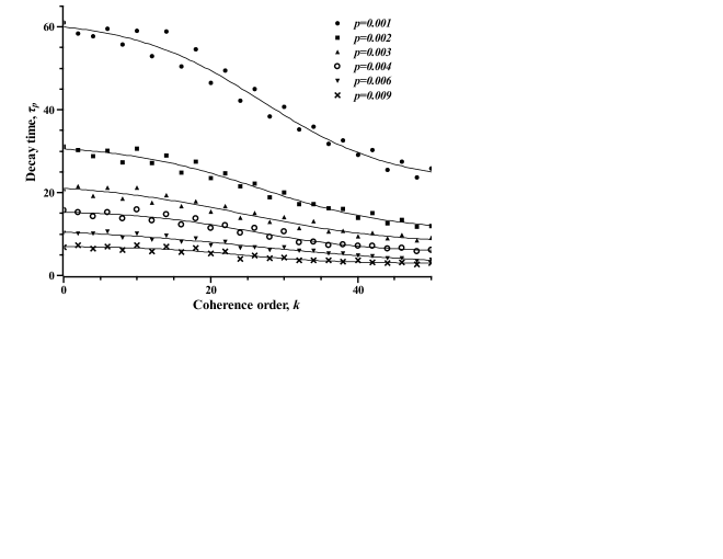
Figure 4: The decay time as a function of the coherence number for spin systems with $N=201$

It is found that this decay may be approximated as follows: $\tau_{p}(k)\approx a_{p}+b_{p}\tanh(d_{p}-c_{p}k)$. Parameters $a_{p}$, $b_{p}$, $c_{p}$, $d_{p}$ have been found by the least square method, see Table I.

p	$a_{p}$	$b_{p}$	$c_{p}$	$d_{p}$
0.001	42.0073	19.7734	0.0565	1.5240
0.002	21.1130	10.5523	0.0543	1.4369
0.003	14.9127	7.4843	0.0472	1.1474
0.004	10.6510	5.0798	0.0606	1.5382
0.006	6.9864	4.7489	0.0358	0.9288
0.009	4.9630	2.0483	0.0778	1.8647

Table 1: The parameters of the approximation $\tau_{p}(k)=a_{p}+b_{p}\tanh(d_{p}-c_{p}k)$ for the spin system with $N=201$

We see that the decay time of the high order coherence intensity depends slightly on its order in accordance with the represented formula. This conclusion is similar to that given in Sec.III.1.1, see eq.(22).

Similar to Sec.III.1.1, we may introduce the cluster of MQ coherences at any time moment $\bar{\tau}$ as a family of such coherences that $\hat{J}^{+}_{k}(\bar{\tau})\geq J_{min}=0.005$. Evolution of the cluster size $N_{c}(\bar{\tau})$ is shown in Fig.5 for different $N$ and $p$. We see that the results of our simulations agree qualitatively with the experimental ones obtained in AS . Namely, there is the period of the coherence cluster growth $0\leq\bar{\tau}\lesssim 1.5$ AS ; BMGP and the period of the cluster decay, $\bar{\tau}\gtrsim 1.5$. Fig.5 demonstrates that the cluster size gets its maximal value at the time moment $\bar{\tau}\approx 1.5$, which is slightly dependent on the both parameters $N$ and $p$. This confirms our assumptions that all spins become embedded in the cluster during the time interval $\tau\sim 1/D$, or $\bar{\tau}\sim 1$. This feature of the cluster growth in the system of equivalent spins is different from that in solids AS . Fig.5 demonstrates also that the maximal size of the cluster increases with the increase in $N$ and slightly decreases with the increase in $p$. The rate of the cluster decay increases with the increase in both $N$ and $p$.

Figure 5: The evolution of the cluster size $N_{c}$ for $N=201$ (solid line), $N=401$ (dashed line), $N=601$ (dotted line) and different $p$; the widths of the lines increase with the decrease of the parameter $p$. The inset shows the periods of the coherence cluster growth and decay at small times.

Comparison of Figs.3 and 5 shows that the case of the modified preparation period is more flexible in preparation of the coherence clusters with the desirable size because of the parameter $p$ which does not appear in Sec.III.1.

IV The conservation law in the model of the dipolar relaxation of MQ NMR coherences

It is worth to emphasize that the appearance of MQ NMR coherences and their relaxation are determined by the same DDI, which is valid in the models both suggested in KS1 ; KS2 ; AS and considered in the previous sections. This leads to some peculiarities of the relaxation process. We show that the sum of areas of the signals of MQ NMR coherences in the frequency domain is not changed in the relaxation process although their maximal amplitudes decrease. For the sake of simplicity, we turn to the case considered in Sec.III.1, where the decay occurs on the evolution period. Then the intensities of MQ NMR coherences are determined by Eq.(17). Performing the Fourier transform of the intensities $J_{k}(\tau,t)$ of Eq.(17) over the time $t$ of the evolution period (we suppose that $J_{k}(\tau,t)=0$ for $t<0$ and $t>T$, where $T$ is the duration of the evolution period)

$${\cal{J}}_{k}(\tau,\omega)=\frac{1}{2\pi}\int_{0}^{T}J_{k}(\tau,t)e^{-i\omega t}dt,$$ (29)

one can find that the area $A_{k}(\tau)$ under ${\cal{J}}_{k}(\tau,\omega)$ in the frequency domain is

$$A_{k}(\tau)=\frac{1}{2\pi}\int_{-\infty}^{\infty}{\cal{J}}_{k}(\tau,\omega)d\omega=$$ (30)

$$\frac{1}{2\pi}\int_{-\infty}^{\infty}d\omega\int_{0}^{T}J_{k}(\tau,t)e^{-i\omega t}dt=$$

$$\frac{1}{2\pi}\int_{0}^{T}J_{k}(\tau,t)dt\int_{-\infty}^{\infty}e^{-i\omega t}d\omega=\frac{1}{2}J_{k}(\tau,0).$$

Then the sum of the areas $A_{k}$ for all MQ NMR coherences can be expressed as follows:

$$\sum_{k}A_{k}(\tau)=\frac{1}{2}\sum_{k}J_{k}(\tau,0).$$ (31)

However, it is known that $\sum_{k}J_{k}(\tau,0)=1$ LHG . Thus, eq.(31) means that the areas $A_{k}(\tau)$ are redistributing during the relaxation process so that their sum is conserved.

Similarly, replacing $t$ with $p$ and $T$ with $1$ in Eqs.(29) and (30) one derives the same conservation law for MQ NMR experiment of Sec.III.2.

The results of this section demonstrate some peculiarities of the used relaxation model.

V Conclusions

Using the numerical methods describing the spin dynamics in large systems of equivalent spins DFFZ1 ; DFFZ2 , we study the decay of MQ NMR coherences in such systems. This decay is caused by the Hamiltonian $\bar{H}_{dz}$ appearing either on the preparation or evolution period of the MQ NMR experiment. Numerical simulations are performed for the systems consisting of 200-600 spins. It is found that the relaxation rate of MQ NMR coherences from the highly correlated spin states increases with the increase in both the MQ NMR order and the number of spins. The dependence of the relaxation time of MQ NMR coherences on the perturbation strength $p$, appearing on the preparation period, is also investigated. We emphasize that the used model KS1 ; KS2 ; AS is the first one for the experimental investigation of the relaxation of the correlated spin clusters of the large size.

It is worth to note that the evolution of the intensities of MQ NMR coherences in the system of equivalent spins is accompanied by the reversion phenomena. Such phenomena were studied both experimentally and numerically RSOPL ; SLAC and the decoherence was considered as the decay of the Loschmidt echo. The reversion phenomena are not considered in this paper.

All numerical simulations have been performed using the resources of the Joint Supercomputer Center (JSCC) of the Russian Academy of Sciences. Authors thank the anonymous referee for the valuable remarks. The work was supported by the Program of the Presidium of Russian Academy of Sciences No.21 ” Foundations of fundamental investigations of nanotechnologies and nanomaterials”.

References

- (1) H.G.Krojanski, and D. Suter, Phys. Rev. Lett. 93, 090501 (2004).
- (2) H.G. Krojanski, and D. Suter, Phys. Rev. Lett. 97, 150503 (2006).
- (3) G.A.Alvarez, and D.Suter, Phys. Rev. Lett. 104, 230403 (2010).
- (4) H.Cho, P.Cappellaro, D.G.Gory, and C.Ramanathan, Phys.Rev. B 74, 224434 (2006)
- (5) J.Baum, M.Munowitz, A.N.Garroway, and A.Pines, J. Chem. Phys, 83, 20015 (1985).
- (6) A.Fedorov, L.Fedichkin, J.Phys.:Condens.Matter 18, 3217 (2006)
- (7) S.I.Doronin, E.B.Fel’dman, I.Ya.Guinzbourg, and I.I.Maximov, Chem. Phys. Lett. 341, 144 (2001).
- (8) V.V.Dobrovitski, H.A.De Raedt, M.I.Katsnelson and B.N.Harmon, Phys. Rev. Lett. 90, 210401 (2003)
- (9) W.X.Zhang, P.Cappellaro, N.Amtler, B.Pepper, D.G.Cory, V.V.Dobrovitski, C.Ramanathan, and L.Viola, Phys. Rev. A 80, 052323 (2009).
- (10) G.A.Álvarez, E.P.Danieli, P.R.Levstein and H.M.Pastawski, Phys.Rev.Lett., 101, 120503 (2008)
- (11) S.I.Doronin, A.V.Fedorova, E.B.Fel’dman, and A.I.Zenchuk, J.Chem.Phys. 131 104109 (2009)
- (12) S.I.Doronin, A.V.Fedorova, E.B.Fel’dman, and A.I.Zenchuk, Phys.Chem.Chem.Phys. 12, 13273 (2010)
- (13) J. Baugh, A. Kleinhammes, D. Han, Q. Wang, and Y. Wu, Science 294, 1505 (2001).
- (14) E. B. Fel’dman, and M. G. Rudavets, J. Exp. Theor. Phys. 98, 207 (2004).
- (15) M. Goldman, Spin Temperature and Nuclear Magnetic Resonance in Solids (Clarendon, Oxford, 1970).
- (16) W.S.Warren, S.Sinton, D.P.Weitekamp and A.Pines, Phys. Rev. Lett. 43, 1791 (1979)
- (17) E.B.Fel’dman, and S.Lacelle, J.Chem.Phys. 107, 7067 (1997)
- (18) L. D. Landau, and E. M. Lifshitz, Course of Theoretical Physics, Vol. 3: Quantum Mechanics: Non-Relativistic Theory (Nauka, Moscow, 1974; Pergamon, New York, 1977).
- (19) H.G.Krojanski, and D. Suter, Phys. Rev. A 74, 062319 (2006)
- (20) D.A.Lathrop, E.S.Handy, and K.K.Gleason, J.Magn.Reson.,Ser.A 111, 161 (1994)
- (21) E.Rufeil-Fiori, C.M.Sanchez, F.Y.Oliva, H.M.Pastawski, and P.R.Levstein, Phys.Rev.A 79, 032324 (2009)
- (22) C.M.Sanchez, P.R.Levstein, R.H.Acosta, and A.K.Chattah, Phys.Rev.A 80, 012328 (2009)