Phase Diagram for a 2-D Two-Temperature Diffusive XY Model

Abstract

Using Monte Carlo simulations, we determine the phase diagram of a diffusive two-temperature conserved order parameter XY model. When the two temperatures are equal the system becomes the equilibrium XY model with the continuous Kosterlitz-Thouless (KT) vortex-antivortex unbinding phase transition. When the two temperatures are unequal the system is driven by an energy flow from the higher temperature heat-bath to the lower temperature one and reaches a far-from-equilibrium steady state. We show that the nonequilibrium phase diagram contains three phases: A homogenous disordered phase and two phases with long range, spin texture order. Two critical lines, representing continuous phase transitions from a homogenous disordered phase to two phases of long range order, meet at the equilibrium KT point. The shape of the nonequilibrium critical lines as they approach the KT point is described by a crossover exponent $\varphi=2.52\pm 0.05$. Finally, we suggest that the transition between the two phases with long-range order is first-order, making the KT-point where all three phases meet a bicritical point.

Much of the research in the statistical physics of nonequilibrium sytems has been directed toward understanding how universal equilibrium critical phenomena are affected by dynamical nonequilibrium perturbations. Field-theoretical studies have indicated that the effects of nonequilibrium dynamics are drastic in systems where detailed balance violation is coupled with conserved anisotropic dynamics Sch95 . In these systems, effective long range interactions can be induced by the local dynamics producing a critical behavior that is remarkably different from the one of the corresponding unperturbed, equilibrium, systems Kat83 ; Kat84 ; Gri85 ; Jan86 ; Leu86 ; Sch93 ; Bas94a ; Bas94b ; Bas94c ; Bas95a ; Bas95b ; Sch96 ; Tau97 ; Sch98 ; Odo04 ; Ris05 ; Zia10 .

In this paper, we present the phase diagram for a two-dimensional two-temperature diffusive conserved order parameter XY model. The system evolves through Kawasaki spin-exchange dynamics Kaw66 . Thus, the dynamics is purely relaxational with no reversible mode couplings, and corresponds to Model B of Ref. Hoh77, . Long range order can exist in nonequilibrium steady states of this system due to the effective long range interactions generated by the anisotropic diffusive dynamics that occurs in that regime. The ordered phase is characterized by the appearance of standing spin waves, or spin textures, oriented along the direction of lower temperature. The system exhibits a nonequilibrium disorder–long-range order transition that is in the same universality class as an equilibrium model with dipole interactions Bas95a ; Tau97 . Note that our model reduces to the equilibrium XY model in the limit where both temperatures are equal. Also, the Mermin-Wagner theorem states that there is no spontaneous symmetry breaking in equilibrium systems with continuous symmetry of the order parameter and dimension $d=2$ Mer66 . Thus, no long-range ordered phase is observed in the two-dimensional equilibrium XY model. However, the equilibrium system still undergoes a transition from quasi-long-range order to disorder characterized by the emergence and unbinding of vortices and antivortices, which is the Kosterlitz-Thouless (KT) transition Kos73 . Hereafter we refer to the quasi-long-range order phase as the KT phase. Since both a KT transition and a disorder–long-range order phase transition occur in the two-dimensional two-temperature XY model, we expect to find a KT–dipole crossover in the phase diagram for this system.

Using results from Monte Carlo simulations, we show that two critical lines representing nonequilibrium disorder–long-range order transition temperatures meet at the equilibrium KT transition temperature. These lines are described by an exponent which we predict to be the universal exponent for KT–dipole crossover. Finally, we argue that, at temperatures below the critical KT temperature, any infinitesimal nonequilibrium perturbation to the system, will produce long-range ordered phases. Thus, the nonequilibrium behavior is very different than that in equilibrium where long-range order is forbidden due to the Mermin-Wagner theorem Bas95a .

Our model consists of a set of two-dimensional spins arranged on a square lattice of rectangular dimensions $L_{x}$ and $L_{y}$. Each spin $\vec{s}_{i}$ is a unit vector. The directions of the spins are evenly distributed from $0$ to $2\pi$ over the lattice, so that their vector sum is null. The total energy of the system is given by the Hamiltonian

$$H=-\sum_{\left\langle ij\right\rangle}\vec{s}_{i}\cdot\vec{s}_{j}\>,$$

where $\left\langle ij\right\rangle$ indicates sum over the nearest neighbor spins on the lattice. The system evolves through Kawasaki exchanges with Metropolis rates Kaw66 ; Met53 . The exchanges along the $x$ and $y$ axes satisfy detailed balance with temperatures $1/\beta_{x}$ and $1/\beta_{y}$, respectively. When $\beta_{x}\neq\beta_{y}$, an energy current flows from the hotter heat bath to the cooler one and detailed balance is no longer satisfied globally. When this is the case, phase transitions occur in nonequilibrium steady states and are characterized by the appearance of a long-wavelength spin texture in the direction with the larger value of $\beta$. In our nonequilbrium simulations, we generally study the case $\beta_{y}<\beta_{x}$, so that the spin texture appears in the $x$ direction. To give a quantitative measure of this ordering, we define the order parameter $\Psi$ as the ensemble averaged arithmetic average of the components of the long-wavelength limit of the structure factor:

$$\Psi=\frac{1}{2}\left[C_{1}\left(\frac{2\pi}{L_{x}},0\right)+C_{2}\left(\frac{2\pi}{L_{x}},0\right)\right]\>,$$

where $C_{n}\left(k_{x},k_{y}\right)$ is the normalized Fourier transform of the $n^{\mathrm{th}}$ component of the spin vectors of our system.

The spatial anisotropy of the system requires an analysis using anisotropic finite size scaling Leu91 . Hence, one must compare systems with sizes that scale in a way that keeps the expression $L_{x}^{1+\Delta}/L_{y}$ constant, where $\Delta$ is the anisotropy exponent. The value $\Delta=1$ has been estimated using renormalization group techniques to first order in a dimensional epsilon expansion Tau99 . Therefore, we performed simulations on systems of sizes $12\times 9$, $16\times 16$, $24\times 36$ and $32\times 64$. Note that there may be higher-order corrections to the value of $\Delta$ that, with this choice of system sizes, would introduce some systematic errors in the data analysis.

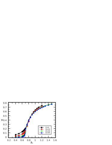
Figure 1: (Color online). Order parameter $\Psi$ vs. $\beta_{x}$ at $\beta_{y}=0$ for different system sizes. The black circles and solid line correspond to a system size of $12\times 9$; the red squares and dashed line correspond to a system size of $16\times 16$; the green diamonds and dotted line correspond to a system size of $24\times 36$; the blue triangles and dashed-dotted line correspond to a system size of $32\times 64$. The plot clearly shows a transition from disorder to order at a $\beta_{x}$ of approximately $0.7$. The error bars are smaller than the symbol size.

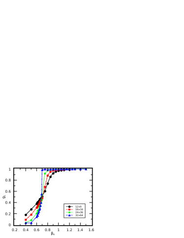
Figure 2: (Color online). Binder’s cumulant $g_{L}$ vs. $\beta_{x}$ at $\beta_{y}=0$ for different system sizes. The black circles and solid line correspond to a system size of $12\times 9$; the red squares and dashed line correspond to a system size of $16\times 16$; the green diamonds and dotted line correspond to a system size of $24\times 36$; the blue triangles and dashed-dotted line correspond to a system size of $32\times 64$. The plots intersect asympotically at $\beta_{x}\approx 0.68$. The error bars are smaller than the symbol size.

We measured $\Psi$ after each Monte Carlo sweep (MCS) during the simulations. After estimating the relaxation time, we determined the ensemble averages $\langle\Psi\rangle$ and $\langle\Psi^{2}\rangle$ over uncorrelated configurations in the steady state. We ran $4\times 10^{6}$, $5\times 10^{6}$, $8\times 10^{7}$ and $10\times 10^{8}$ MCS for the system sizes $12\times 9$, $16\times 16$, $24\times 36$ and $32\times 64$, respectively. Integrated autocorrelation times ranged from roughly 200 MCS for the smallest system to roughly 1200 MCS for the largest system.

Our simulations reveal that long-range ordered states occur when $\beta_{y}$ is sufficiently small and $\beta_{x}$ is sufficiently large or viceversa, by symmetry. Note that the $\beta_{x}$–$\beta_{y}$ phase diagram for this system is symmetric about the diagonal since interchanging these temperatures is equivalent to simply renaming the axes of the lattice. Thus, we study the ordering process only in the $\beta_{y}<\beta_{x}$ region.

Figure 1 shows the value of $\Psi$ as a function of $\beta_{x}$ with $\beta_{y}=0$ for different system sizes. The data clearly show ordering occuring at $\beta_{x}\approx 0.7$. Graphs showing similar critical behavior were produced for each simulated value of $\beta_{y}$. We achieved more precise estimates of the disorder–order transition temperatures by measuring the crossing point of Binder’s cumulant $g_{L}\equiv 3-2\left(\left\langle\Psi^{2}\right\rangle/{\langle\Psi\rangle}^{2}\right)$ Lan00 . As expected for a continuous phase transition, the values of $g_{L}$ for different system sizes cross at the critical point $\beta_{x_{\mathrm{c}}}$, as shown in Fig. 2. This allowed us to measure the critical $\beta_{x}$ for $\beta_{y}$ values of $-0.9$, $-0.75$, $-0.6$, $-0.3$, 0, $0.3$, $0.6$, $0.75$, $0.9$ and 1.

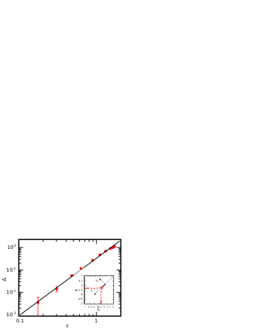
Figure 3: (Color online). Power-law fit of the dependence of $\delta$ on $\varepsilon$ for the measured critical points. The points lying on a straight line on a double logarithmic plot imply $\delta\sim\varepsilon^{\varphi}$. The slope of the line corresponds to the universal crossover exponent $\varphi$. We measure $\varphi=2.52\pm 0.05$. The inset shows the geometric representation of the $\varepsilon-\delta$ coordinates.

The locations of the transition points can be parametrized in terms of the quantities $\varepsilon=\left(2\beta_{KT}-\beta_{x_{c}}-\beta_{y_{c}}\right)/\sqrt{2}$ and $\delta=\left(\beta_{x_{c}}-\beta_{y_{c}}\right)/\sqrt{2}$. The result of such parametrization is shown in a log-log plot in Fig. 3. The possibility of fitting the data to a straight line implies they obey the power law $\delta\sim\varepsilon^{\varphi}$. The slope of this line allows us to estimate the crossover exponent as $\varphi=2.52\pm 0.05$.

Figure 4 shows the phase diagram for the model. The insets in the figure show the alignment of the spin textures associated with ordered states. The two critical lines representing the nonequilibrium disorder–long range order transitions meet at a temperature $1/\beta_{c}\approx 0.89$. This is the same as the KT critical temperature Gup92 , leading us to conclude that the ordered regions of the diagram meet at a line corresponding to the low temperature equilibrium KT phase.

Monte Carlo simulations were also used to investigate the low temperature behavior of our system near equilibrium. We measured the time evolution of the difference $\delta\Psi$ between the order parameters for the $x$ and $y$ directions. This was done while varying $\beta_{x}$ and $\beta_{y}$ so that, as time (MCS) progressed, we moved perpendicularly across the equilibrium line from one long-range ordered region to the other. Hysteresis was clearly observed for square systems smaller than $32\times 32$, indicating that the equilibrium line may also be a line of first order transitions from order in one direction to order in the other.

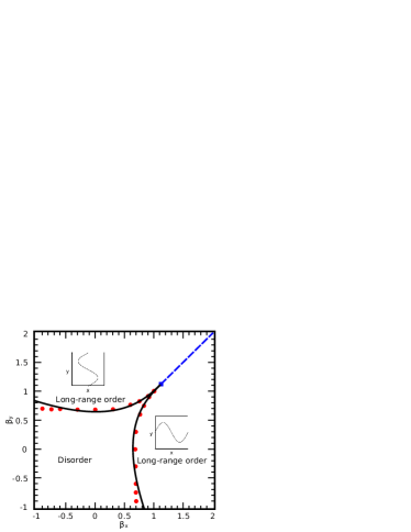
Figure 4: (Color online). Phase diagram for the two-dimensional two-temperature XY model. The red points are actual measurements of the nonequilibrium transition temperatures between disorder and long-range order phases. The two solid black critical lines are drawn with a crossover exponent $\varphi=2.52$ to fit the points. The blue dashed line corresponds to the equilibrium KT phase. The blue square corresponds to the KT transition temperature. The insets show schematic drawings of spin textures in the ordered state. The error bars are smaller than the symbol size.

However, for larger system sizes, a different, glassy-type of behavior was observed. The quantity $\delta\Psi$ did not switch from a large positive (negative) value to a large negative (positive) value, as in a hysteresis loop, but stayed at a value of approximately 0 after crossing the equilibrium line. The actual system configurations where $\delta\Psi\approx 0$ were investigated, and we observed columns of ordered vectors, pointing in roughly the same direction, between columns of disordered vectors.

We note that a similar “striped” configuration was observed after deep quenches from the high temperature disordered phase to a low temperature ordered phase. In the steady state simulations described above, we avoided these striped configurations in favor of long wavelength spin textures by starting the simulations in the steady state configuration of a temperature very close to the one currently being simulated; this process was continued for monotonically decreasing temperatures from the disordered phase to the ordered phase. Thus, quenching of the system to a striped configuration was avoided.

We believe the striped configuration to be a metastable state that can be found in finite-sized systems with anisotropic nonequilibrium dynamics, e.g. a driven Ising model Hur02 . We caution however that in the case of a driven diffusive Ising model, such striped configurations are stable in the thermodynamic limit $L\rightarrow\infty$ Lev01 ; Zia00 . In particular, if $L_{\parallel}$ is the dimension of the drive and $L_{\perp}$ the other dimension, “wide” systems ($L_{\perp}>L_{\parallel}$) and square systems support stable striped configurations, while “narrow” systems ($L_{\parallel}\gg L_{\perp}$) support stable long-range ordered configurations (a single stripe in the case of the Ising model). In light of these results for the driven Ising model, we note that it is possible that the striped configurations in our model may represent true stable states, particularly for the large square systems used in the simulations exploring the low-temperature region.

In any case, these striped configurations do not indicate an extended KT phase in the low temperature region since the KT phase, characterized by the appearance of vortices, is entirely different from the long-range ordered phase or the striped phase. Thus, the phase diagram is drawn to indicate that infinitesimal non-equilibrium perturbations to the dynamics of the system cause completely different system behavior at temperatures below the KT transition temperature.

This is consistent with what can be inferred from the following argument. Consider the Langevin equation for model B with a two-component order parameter $\vec{\eta}$:

$$\partial_{t}\vec{\eta}=\lambda\nabla^{2}\left[\left(-\nabla^{2}+\tau\right)\vec{\eta}+\frac{1}{6}g\vec{\eta}\eta^{2}\right]+\vec{\xi}\>,$$

where $\vec{\delta}$ is the order parameter field, $g$ and $\lambda$ are generic constants, $\vec{\xi}$ is a Gaussian noise term and $\tau\equiv\frac{T-T_{c}}{T_{c}}$ is the reduced temperature. To account for the system having two different temperatures, the operators, the parameters and the noise term are split into $x$ and $y$ components:

$$\begin{split}\partial_{t}\vec{\eta}=&\lambda\left\{\partial_{x}^{2}\left[\left(-\partial_{x}^{2}+\tau_{x}\right)\vec{\eta}+\frac{1}{6}g_{x}\vec{\eta}\eta^{2}\right]+\right.\\ &\left.\partial_{y}^{2}\left[\left(-\partial_{y}^{2}+\tau_{y}\right)\vec{\eta}+\frac{1}{6}g_{y}\vec{\eta}\eta^{2}\right]\right\}+\\ &\xi_{x}\hat{x}+\xi_{y}\hat{y}+2\partial_{x}^{2}\partial_{y}^{2}\vec{\eta}\>,\end{split}$$

where $\hat{x}$ and $\hat{y}$ are the unit vectors in the $x$ and $y$ directions, respectively. To describe the system below criticality close to the equilibrium line, both $\tau$s should be negative Sch95 . This means that the system is unstable with respect to perturbations in both directions. The case $\tau_{x}=\tau_{y}$ corresponds to the equilibrium model, in which the instability has the same importance in both directions. However, any nonequilibrium perturbation will cause the instability to become stronger in one of the two directions, thus generating effective long range correlations in the direction corresponding to the lower $\tau$. The possibility of an extended KT phase is ruled out by the established result that, for large enough systems, the contribution to the correlation between far away spins due to vortices is vanishingly small Kos74 . This means that any long range interaction, however small, is enough to make vortices unimportant in the description of the system. Consequently, the equilibrium KT phase is destroyed by any nonequilibrium perturbations.

In conclusion, we determined the phase diagram for a two-dimensional two-temperature conserved order parameter XY model. The system, whose evolution happens through Kawasaki spin exchanges, has lines of continuous phase transition between ordered states, characterized by the appearance of spin textures in the direction of the lower temperature, and a disordered state. These lines meet at the equilibrium KT point, corresponding to a KT transition in the equilibrium model. We measured the crossover universal critical exponent $\varphi$ for this transition, finding the value $\varphi=2.52\pm 0.05$. For temperatures lower than the KT point, the equilibrium line on the phase diagram is a line of first order transition between the ordered states, with the direction of the spin textures changing. We provided an argument validating our finding and excluding the possibility of an extended KT phase below criticality.

- (1) B. Schmittmann and R. K. P. Zia, in Phase Transitions and Critical Phenomena, edited by C. Domb and J. L. Lebowitz (Academic Press, New York, 1995) Vol. 17.
- (2) S. Katz, J. L. Lebowitz, and H. Spohn, Phys. Rev. B 28, 1655 (1983).
- (3) S. Katz, J. L. Lebowitz, and H. Spohn, J. Stat. Phys. 34, 497 (1984).
- (4) G. Grinstein, C. Jayaprakash, and Y. He, Phys. Rev. Lett. 55, 2527 (1985).
- (5) H. K. Janssen and B. Schmittmann, Z. Phys. B 64, 503 (1986).
- (6) K.-t. Leung and J. L. Cardy, J. Stat. Phys. 44, 567 (1986); 45, 1087(1986).
- (7) B. Schmittmann, EPL 24, 109 (1993).
- (8) K. E. Bassler and Z. Rácz, Phys. Rev. Lett. 73, 1320 (1994).
- (9) K. E. Bassler and B. Schmittmann, Phys. Rev. Lett. 73, 3343 (1994); 74, 3501 (1995).
- (10) K. E. Bassler and R. K. P. Zia, Phys. Rev. E 49, 5871 (1994).
- (11) K. E. Bassler and Z. Rácz, Phys. Rev. E 52, R9 (1995).
- (12) K. E. Bassler and R. K. P. Zia, J. Stat. Phys. 80, 499 (1995).
- (13) B. Schmittmann and K. E. Bassler, Phys. Rev. Lett. 77, 3581 (1996).
- (14) U. C. Täuber and Z. Rácz, Phys. Rev. E 55, 4120 (1997).
- (15) B. Schmittmann and R. K. P. Zia, J. Stat. Phys. 91, 525 (1998).
- (16) G. Ódor, Rev. Mod. Phys. 76, 663 (2004).
- (17) T. Risler, J. Prost, and F. Jülicher, Phys. Rev. E 72, 016130 (2005).
- (18) R. K. P. Zia, J. Stat. Phys. 138, 20 (2010).
- (19) K. Kawasaki, Phys. Rev. 145, 224 (1966).
- (20) P. C. Hohenberg and B. I. Halperin, Rev. Mod. Phys. 49, 435 (1977).
- (21) N. D. Mermin and H. Wagner, Phys. Rev. Lett. 17, 1133 (1966).
- (22) J. M. Kosterlitz and D. J. Thouless, J. Phys. C 6, 1181 (1973).
- (23) N. Metropolis et al., J. Chem. Phys. 21, 1087 (1953).
- (24) K.-t. Leung, Phys. Rev. Lett. 66, 453 (1991).
- (25) D. P. Landau and K. Binder, A Guide to Monte Carlo Simulations in Statistical Physics, (Cambridge University Press, Cambridge, England, 2000).
- (26) U. C. Täuber, J. E. Santos, and Z. Rácz, Eur. Phys. J. B 7, 309 (1999).
- (27) R. Gupta and C. F. Baillie, Phys. Rev. B 45, 2883 (1992).
- (28) P. I. Hurtado, J. Marro, and E. V. Albano, EPL 59, 14 (2002).
- (29) R. K. P. Zia, L. B. Shaw, and B. Schmittmann, Physica A 279, 60 (2000).
- (30) E. Levine, Y. Kafri, and D. Mukamel, Phys. Rev. E 64, 026105 (2001).
- (31) J. M. Kosterlitz, J. Phys. C 7, 1046 (1974).