Type II-P Supernovae as Standard Candles: The SDSS-II Sample Revisited

Abstract

We revisit the observed correlation between H${\beta}$ and Fe II velocities for Type II-P supernovae (SNe II-P) using 28 optical spectra of 13 SNe II-P and demonstrate that it is well modeled by a linear relation with a dispersion of about 300 km s^-1. Using this correlation, we reanalyze the publicly available sample of SNe II-P compiled by D’Andrea et al. and find a Hubble diagram with an intrinsic scatter of 11% in distance, which is nearly as tight as that measured before their sample is added to the existing set. The larger scatter reported in their work is found to be systematic, and most of it can be alleviated by measuring H${\beta}$ rather than Fe II velocities, due to the low signal-to-noise ratios and early epochs at which many of the optical spectra were obtained. Their sample, while supporting the mounting evidence that SNe II-P are good cosmic rulers, is biased toward intrinsically brighter objects and is not a suitable set to improve upon SN II-P correlation parameters. This will await a dedicated survey.

1. Introduction

Type II supernovae (SNe) that undergo a long, bright, flat phase in photometric evolution are commonly referred to as plateau SNe (SNe II-P). These have been shown over the past decade to be good “standardizable candles,” and potential cosmological probes, in a manner similar to that of their more famous cousins, SNe Ia. Hamuy & Pinto (2002) were the first to demonstrate this empirical “standardizable candle method” (SCM), a technique which was later streamlined and applied to larger samples by Nugent et al. (2006, hereafter N06) and Poznanski et al. (2009a, hereafter P09); see also Olivares et al. (2010).

P09 used a sample of 34 SNe II-P to constrain the three parameters that define the correlation: a reference absolute magnitude in the $I$ band, a velocity term that is correlated with the luminosity during the plateau, and a color term that minimizes the contribution from intrinsic color inhomogeneity as well as from dust extinction. The resulting intrinsic scatter in the Hubble diagram was found to be 0.22 mag, which is equivalent to about 10% in distance, similar to the result of N06 despite the larger sample. Since the samples used by N06 and P09 are dominated by nearby SNe that sport large distance uncertainties due to peculiar velocities, a robust derivation of the SCM parameters, together with a determination of its potential power, requires a set of SNe II-P in the Hubble flow.

Recently, D’Andrea et al. (2010, hereafter D10) presented such a sample of 15 SNe II-P in the Hubble flow from the Sloan Digital Sky Survey II (SDSS-II) SN survey, albeit obtained during a project that was focused on SNe Ia. The SCM method relies on photospheric velocities measured from the Fe II $\lambda$5169 absorption line during the plateau phase, specifically about 50 days past explosion. As noted by D10, however, the optical spectra of their SNe II-P are usually of low signal-to-noise ratio (S/N) and taken at an early epoch, when Fe II lines are not fully developed. This observation strategy, while complicating the application of the SCM method to SNe II-P, was dictated by the main purpose of their survey, which was to identify SNe Ia and measure their redshifts in order to use them as distance indicators (Kessler et al. 2009). D10 find that adding their sample to those analyzed previously increases the scatter significantly, to 15% in distance. This points to a failure of the data, method, or underlying model.

While D10 conscientiously explore many possible sources for this scatter, we show below that most of it is due to a systematic offset, and could be explained by two effects: the method used to determine the photospheric velocities, and an observational bias. In §2 we rederive photospheric velocities for their sample using H${\beta}$ absorption lines, as applied by N06 to their sample of higher redshift SNe. We calibrate the relation between H${\beta}$ velocities and the standard Fe II velocities in §3. In §4 we update the Hubble diagram and discuss the specific selection effects that bias the SDSS-II sample.

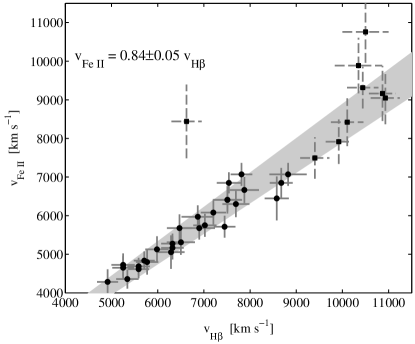
Figure 1.— Velocities determined from the absorption minima of H${\beta}$ $\lambda$4861 and Fe II $\lambda$5169 using 28 spectra of 13 SNe II-P at phases of 5 to 40 days after explosion. The shaded area marks the 1$\sigma$ region for the derived correlation, $v_{\rm Fe~{}II}=(0.84\pm 0.05)\,v_{\rm H\beta}$. Fe II velocities can be well determined using H${\beta}$, which is easier to detect in early-phase and low-S/N spectra. Squares with dashed error bars mark Fe II velocities derived for objects with very high H${\beta}$ velocities using Eq. 2 of N06. The outlier at $v_{\rm Fe~{}II}\approx 8,400$ km s^-1 is from a very early spectrum (2 days past explosion) of the low-luminosity, low-velocity SN 2005cs.

2. Photospheric Velocities

In order to derive photospheric velocities, D10 apply to their spectra the algorithm developed by P09. Briefly, using the “SN Identification Code” (SNID; Blondin & Tonry 2007), the spectra are cross-correlated with a library of high-S/N templates for which Fe II velocities can be measured precisely. P09 successfully applied this method to 19 nearby SNe II-P that typically had a few high-S/N spectra per object, many of them near day 50 after explosion. D10 correctly point out that this method may not be applicable to their sample, due to the early epoch at which they were obtained and their low S/N. The Fe II lines usually become fully developed after a few weeks past explosion. Even at later times those lines are often weak, making velocity derivation from low-S/N spectra problematic.

We rederive the velocities for the SDSS-II sample using another method, and find values that are typically different from those of D10. These in turn improve the scatter in the Hubble diagram, as demonstrated in §4. N06 showed that there is a correlation between the velocities measured from H${\beta}$ $\lambda$4861 and those derived from Fe II $\lambda$5169. In the next section we improve the determination of that correlation using many more objects and spectra.

We obtain the photospheric velocities for the SDSS-II sample as follows. From each spectrum we measure the H${\beta}$ velocity, and where feasible, the Fe II velocity. This is done by finding the minimum of the absorption line. When the S/N is too low we smooth the spectra with a Savitzky-Golay filter (which is similar to a running mean; Savitzky & Golay 1964). For most of the SDSS-II spectra, Fe II $\lambda$5169 is either undeveloped or buried in the noise. The H${\beta}$ velocities are translated to equivalent Fe II velocities using the relation found in §3 (with the uncertainty in that relationship folded in quadrature). For every spectrum that does have a direct Fe II velocity measurement, we calculate a weighted mean between the direct and indirect values. These velocities and uncertainties are then propagated to day 50 (as was done by N06, P09, and D10) and listed in Table 1.

Table 1Day-50 Velocities for the SDSS-II SNe II-P

IAU Name	D10 (km s-1)	H${\beta}$ based (km s-1)
SN 2007ld	4110(570)	3970(660)
SN 2006iw	4490(160)	4660(270)
SN 2007lb	3950(340)	4080(420)
SN 2007lj	4220(460)	4110(450)
SN 2006jl	5560(310)	4780(350)
SN 2007lx	3900(820)	4170(910)
SN 2007nw	4290(750)	4830(840)
SN 2006kv	3640(620)	4050(950)
SN 2007kw	3930(460)	4990(1060)
SN 2006gq	3400(150)	3790(440)
SN 2007ky	3510(420)	4060(480)
SN 18321	5060(640)	5820(700)
SN 2006kn	4220(440)	5000(590)
SN 2007kz	4380(320)	5490(370)
SN 2007nr	4430(350)	4900(590)

Note. — Values in parentheses are 1$\sigma$ uncertainties.

3. Correlation between H${\beta}$ and Fe II Velocities

N06 propose an alternative velocity proxy to Fe II, using the H${\beta}$ absorption line that is both present early and significantly more prominent. We repeat the analysis of N06 using the much larger sample of P09 and derive a new relation between the two velocities.

We use 28 spectra of 13 SNe II-P that span ages of 5 to 40 days past explosion; both lines are readily identifiable in all of the spectra. We restrict ourselves to spectra obtained prior to day 40, since at later times Fe II $\lambda$5169 is at least as strong as H${\beta}$, which also becomes blended with other lines that can bias the velocity measurement. We measure the velocities as described for the SDSS-II SNe in §2.

As seen in Figure 1, we find a robust ($\chi^{2}/{\rm dof}\approx 1$) linear correlation that can be represented as $v_{\rm Fe~{}II}=(0.84\pm 0.05)\,v_{\rm H\beta}$. The uncertainty is equivalent to an additional error of about 200–400 km s^-1 over the relevant range of velocities. While this relation is somewhat different from the one derived by N06, in practice it gives similar results for the range of velocities probed by the SDSS-II sample.

Since there are very few objects in the P09 sample having velocities higher than 8,000 km s^-1 in which both lines are well developed, we add to Figure 1 nine early-epoch, high-velocity spectra where the Fe II lines are not detected. In order to approximate the Fe II velocity at those times, we use the velocity derived for these objects at day 50 in P09, and propagate them to the correct epoch using Equation 2 of N06 which models the time evolution of Fe II velocities. Most of the additional spectra seem to agree with the relationship derived above, with two notable exceptions. One is SN 2005cs (2 days past explosion) with a derived Fe II velocity which is much too high. This object was a low-luminosity, low-velocity SN II-P, and is of little relevance to nonlocal samples. The second exception is that at H${\beta}$ velocities higher than 10,000 km s^-1 the scatter increases significantly. This may be due to a combination of line blending at these high velocities, combined with very blue continua that make absorption minima harder to define and measure. All of the SNe in the D10 sample have a spectrum with H${\beta}$ velocity smaller than 10,000 km s^-1. While these exceptions are not relevant to the reanalysis of the D10 sample, one should be cautious and remember that this correlation may break down for spectra with extremely high or low velocities.

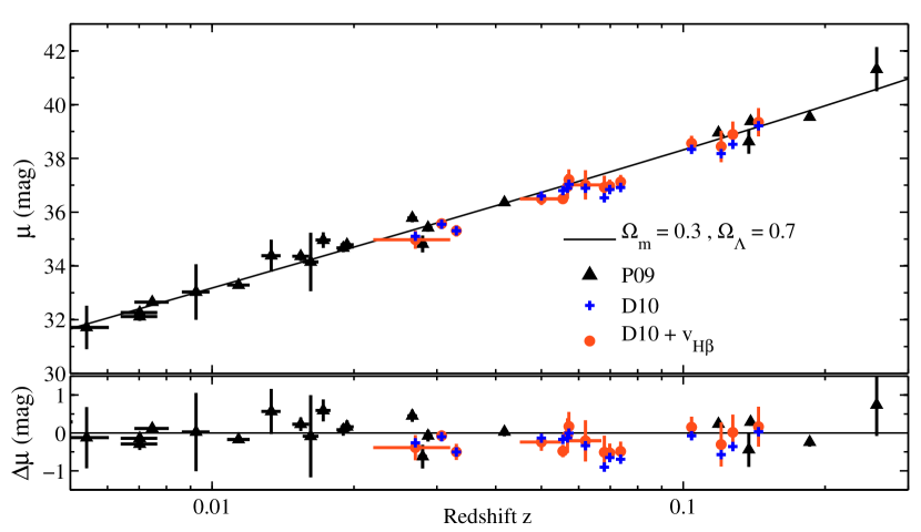
Figure 2.— Hubble diagram (top) and residuals from the standard concordance cosmological model (bottom) for the P09 sample (black triangles), the D10 sample (blue crosses; uncertainties omitted for clarity), and the D10 sample with corrected velocities (orange filled circles). The standard cosmological model (line) is shown to guide the eye. The velocity correction mostly shifts the D10 sample to fainter luminosities, and hence to larger “apparent distances,” more consistent with the Hubble law. For clarity we show here only the sample of 36 SNe II-P at redshifts $z>0.005$, where peculiar-velocity uncertainties are less dominant.

4. Hubble Diagram

When minimizing the “cost function” (Equation 4 of P09) in order to determine the best-fit parameters, P09 find an intrinsic scatter of 0.22 mag (D10 measure it to be 0.20 mag when minimizing a slightly different function), which is equivalent to $\sim$10% in distance, similar to the result of N06. D10 report an increase to 0.29 mag (which we measure to be 0.32 mag) when adding the SDSS-II sample, which is about 50% more scatter. An important clue to the source of this additional dispersion is provided by Figure 5 of D10, which clearly shows that the SDSS-II SNe are systematically offset from the Hubble law, with all but one of them falling below the line. In fact, the scatter is reduced significantly by artificially dimming the SDSS-II SNe by 0.4 mag, ending up even smaller than that reported by P09.

We repeat the analysis of D10 using all of their data, except for the velocities and their respective uncertainties, where we substitute those we find in §2. As can be seen in Figure 2, this eliminates a substantial fraction of the systematic offset, which in turn reduces the intrinsic scatter to 0.25 mag (11% in distance), only slightly higher than without this sample. Our best-fit parameters for the combined sample are nearly identical to those of P09, except for the reference absolute magnitude which is 0.1 mag brighter for the combined sample.

Deriving the parameters using only the SDSS-II sample, we still find preferred values for the correlation coefficients that are offset from those of P09. The SDSS-II SNe appear to be predominantly overluminous, and favor a small value for the velocity correlation coefficient. Following the suggestion made by D10, we show below that this is largely due to an observational bias arising from the SDSS-II follow-up criteria.

We have performed Monte Carlo simulations, starting from a SN population that mimics the properties of the P09 sample, to which we apply various observational cuts. For these simulated samples we then compute the best-fit correlation parameters. We find that a simple magnitude cut cannot produce such biased values. However, selecting objects that are intrinsically brighter skews the parameter derivation in the right direction. Folding in the larger velocity uncertainties allows us to reproduce the bias toward luminous SNe with little correlation. Indeed, when one selects only luminous SNe, it is not surprising that the best-fit reference absolute magnitude is brighter, and the correlation parameters smaller — thus pointing toward a weaker link between luminosity and velocity. The lack of statistical power of such a sample is reflected by the fact that the parameters derived from the combined set are almost identical to those recovered without including the SDSS-II sample. Because the SDSS-II sample does not cover a substantial region of parameter space, it cannot significantly constrain the SCM parameters.

D10 mention that the contrast between a SN and its host galaxy was a selection criterion for spectroscopic follow-up observations. This was obviously done to increase the efficiency of their spectroscopic observing runs and the number of SNe Ia they find. Unlike a regular Malmquist bias that skews the distribution near the detection limit of the survey, such a criterion selects intrinsically bright objects, independent of redshift. This is evident from the very different luminosity functions of the two samples (Fig. 7 of D10). Figure 3 shows that nearly half of the SDSS-II SNe are brighter than their host galaxies up to a factor of a few, unlike the samples of P09 and N06 that are consistently fainter than their hosts. A better understanding of the SCM relation, based on larger, less biased samples, will allow a careful determination of the various potential biases, providing a crucial component for constraining cosmological parameters.

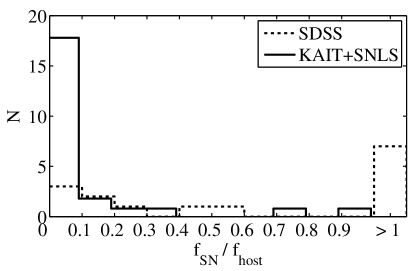
Figure 3.— Approximate $I$-band flux ratios (SN/host galaxy) for the Katzman Automatic Imaging Telescope (KAIT; P09) and Supernova Legacy Survey (SNLS; N06) samples (solid line) and for the SDSS-II sample from D10 (dotted line). About half of the SDSS-II SNe are brighter than their hosts galaxies, a selection effect that removes intrinsically faint objects and skews the estimation of correlation parameters.

5. Conclusions

We find that when measuring expansion velocities for the SDSS-II sample of SNe II-P by using H${\beta}$, the SCM correlation gives a tight Hubble diagram, with a scatter of $\sim$11% in distance. This is comparable to the scatter obtained with previous samples of SNe II-P, despite a systematic offset among the SDSS-II objects, which is probably due to a strong bias favoring intrinsically bright SNe.

Our analysis shows that H${\beta}$ velocities correlate well with those derived from Fe II lines, with a scatter of about 300 km s^-1, enabling the use of early-time spectra and data having low S/N.

The SCM parameters and the true tightness of the correlation remain to be tested with high-quality Hubble-flow data. We are currently compiling such a set of SNe II-P from the Palomar Transient Factory (Rau et al. 2009; Law et al. 2009; Poznanski et al. 2009b), where cosmology with SNe II-P is one of the key projects and should lead to less biased samples.

References

- Blondin & Tonry (2007) Blondin, S., & Tonry, J. L. 2007, ApJ, 666, 1024
- D’Andrea et al. (2010) D’Andrea, C. B., et al. 2010, ApJ, 708, 661 (D10)
- Hamuy & Pinto (2002) Hamuy, M., & Pinto, P. A. 2002, ApJ, 566, L63
- Kessler et al. (2009) Kessler, R., et al. 2009, ApJS, 185, 32
- Law et al. (2009) Law, N. M., et al. 2009, PASP, 121, 1395
- Nugent et al. (2006) Nugent, P., et al. 2006, ApJ, 645, 841 (N06)
- Olivares et al. (2010) Olivares, F., et al. 2010, ApJ, 715, 833
- Poznanski et al. (2009a) Poznanski, D., et al. 2009a, ApJ, 694, 1067 (P09)
- Poznanski et al. (2009b) Poznanski, D., et al. 2009b, BAAS, 213, 469.09
- Rau et al. (2009) Rau, A., et al. 2009, PASP, 121, 1334
- Savitzky & Golay (1964) Savitzky, A., & Golay, M. J. E. 1964, Analytical Chemistry, 36, 1627