A Time-Asymmetric Process in Central Force Scatterings

Abstract

This article puts forth a process applicable to central force scatterings. Under certain assumptions, we show that in attractive force fields a high speed particle with a small mass speeding through space, statistically loses energy by colliding softly with large masses that move slowly and randomly. Furthermore, we show that the opposite holds in repulsive force fields: the small particle statistically gains energy. This effect is small and is mainly due to asymmetric energy exchange of the transverse (i.e., perpendicular) collisions. We derive a formula that quantifies this effect (Eq.(12)). We then put this work in a broader statistical context and discuss its consistency with established results.

Dynamical Description- In addition to the well known gravitational and Coulomb, nearly all other interactions in nature such as intermolecular forces and interaction of vortices in superconductors are central LJones ; blatter ; ramis_roessler . In conservative fields, the central force on each particle can be derived from a potential function by $F=-\mathbf{\mathbf{\nabla}}V\left(r\right)$ where $V(r)=\frac{\alpha}{r^{k}}$; $\alpha$ is the strength of the interaction depending on the parameters of the problem, $k$ defines the range of the interaction remark1 . $\alpha<0$ and $\alpha>0$ correspond to attractive and repulsive force fields respectively.

In many applications, statistical inferences resulting from many-body interaction is approximated by series of two-body scatterings chandra1 ; chandra2 ; chandra3 ; tyson . While there is an active frontier of numerical work on many-body simulations Hut ; Henon , there are still interesting statistical inferences that can be derived from close analysis of two-body collisions.

In this paper we study a fast small mass passing through a dilute system of randomly moving central forces, where changes in the state of the small mass can be well approximated by a series of two-body scatterings. We report on a net small effect in the statistical change of the energy of the small mass (Eqs.(11, 12)).

Consider a scattering, in the lab frame, between two interacting particles $m_{1}$ and $m_{2}$ where $m_{2}$ is much lighter ($m_{2}\ll m_{1}$) yet much faster ($v_{2}\gg v_{1}$) than $m_{1}$ but nevertheless $m_{1}v_{1}^{2}\gg m_{2}v_{2}^{2}$. This in particular implies $m_{1}v_{1}\gg m_{2}v_{2}$. For example, one can visualize a small comet ($m_{2}$) undergoing a small angle scattering in the gravitational field of the planet Jupiter ($m_{1}$). In a typical scattering $m_{1}$ is initially moving. The questions we are interested in investigating are: What statistically invariant features are shared by series of such scatterings in randomly moving central force fields? Would many such small angle scatterings have a net effect on the energy of $m_{2}$ under the assumptions stated above?

Statistical properties based on probabilities of encounters where collisions are heads-on have been extensively studied as in the Fermi acceleration mechanism fermi . In contrast, the main contribution to the effect herein is from transverse collisions, where the trajectory of the massive particle, roughly speaking, is perpendicular to that of the small particle during the effective scattering.

In the remainder of this section we heuristically describe the effect; in the next section we analytically prove it and derive a formula. Lastly, we discuss it in a larger statistical context. Throughout, we refer to the Supplementary Material SM for details when needed.

For the sake of concreteness take the potential to be attractive for now. Let us consider two extreme cases that would convey the gist of what underlies this work. In the first case the massive particle, $m_{1}$, slowly and transversely veers away from the trajectory of $m_{2}$ that is speeding by. In the second case, $m_{1}$ slowly and transversely approaches the trajectory of $m_{2}$.

In the first case where $m_{1}$ is moving away, $m_{2}$ falls into the potential well of $m_{1}$ and so long as it is approaching the point of minimum distance it gains kinetic energy. After passing this point, $m_{2}$ starts climbing up the potential well and pays back the gained kinetic energy by restoring it into the potential energy of the two-body system. However, on the way out it climbs a potential well that is effectively smaller than the one it fell into as $m_{1}$ is on average farther away from it ($\Delta E_{\mbox{recede}}$ in Fig. 1). Therefore, in the case that the large mass is transversely receding away, the small particle emerges with a gain in the kinetic energy i.e., $\frac{1}{2}m_{2}|v_{m_{2}}|_{-\infty}^{2}<\frac{1}{2}m_{2}|v_{m_{2}}|_{+\infty}^{2}$.

The exact opposite effect holds in the second case, where $m_{1}$ is moving towards $m_{2}$. In this case, $m_{2}$ enters the potential well set up by $m_{1}$ and, as in the previous case, gains kinetic energy so long as it is approaching the minimum distance between the two masses. However, on the way out it faces a more demanding climb as $m_{1}$ is on average closer to it and the potential well is steeper and deeper than before ($\Delta E_{\mbox{approach}}$ in Fig. 1). Therefore, in the case that the large mass is transversely approaching, the small particle emerges with a loss in the kinetic energy i.e. $\frac{1}{2}m_{2}|v_{m_{2}}|_{-\infty}^{2}>\frac{1}{2}m_{2}|v_{m_{2}}|_{+\infty}^{2}$ .

The point however is that the two cases are not symmetric. The decreasing of the magnitude of the force with distance breaks the symmetry between the two cases. This is shown in Fig. 1: In an attractive force field, $m_{2}$ has a greater loss (in magnitude) of energy when $m_{1}$ approaches it than a gain (in magnitude) when $m_{1}$ recedes away from it. This asymmetry, deduced from dynamical principles, has consequences for the statistical mechanics of $m_{2}$.

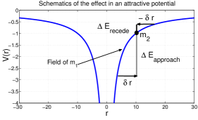
Figure 1: $V(r)$ set up by $m_{1}$ shown in blue with $\alpha<0$. The small mass $m_{2}$ is shown as a black circle. When $m_{1}$ moves to the right (approaches $m_{2}$) by $\delta r$, during the effective scattering, $m_{2}$ loses $\Delta E_{\mbox{approach}}$ of energy. When $m_{1}$ is moving to the left (away from $m_{2}$) by the same amount $\delta r$, $m_{2}$ gains $\Delta E_{\mbox{recede}}$ of energy. Note: $|\Delta E_{\mbox{approach}}|>|\Delta E_{\mbox{recede}}|$.

In repulsive force fields, $\alpha>0$, the potential in Fig. 1 flips about the horizontal axis. Therefore the phenomenology is the exact opposite. Namely, the particle has a larger gain than loss.

So far we have described a purely dynamical phenomena where $m_{2}$ collides softly and transversely with $m_{1}$ where a very fast small particle (e.g., an electron) zips through a dilute soup of big masses (e.g, massive ions or stars in a galaxy) that randomly either approach it or move away from it. The small mass statistically loses (gains) energy to (from) the big masses when the force fields are attractive (repulsive).

We are considering an standard elastic collision L_Mechanics . Let $\mathbf{v_{1}}$ and $\mathbf{\mathbf{\mathbf{v}}_{2}}$ be the velocities of $m_{1}$ and $m_{2}$ respectively in the lab frame and let $\mathbf{V}=\mathbf{v_{2}}-\mathbf{\mathbf{v}_{1}}$. Denote by $\mathbf{n}_{0}^{+}$ the unit vector in the direction of the velocity of $m_{2}$ in the center of mass after the collision which is parallel to $\mathbf{V}$. Then the velocities of the two particles after the collision (distinguished by primes) are

$$\mathbf{v_{1}^{\prime}} = -m_{2}V\mathbf{\mathbf{n}_{0}^{+}}/(m_{1}+m_{2})+\mathbf{V_{g}},$$ (1)

$$\mathbf{v_{2}^{\prime}} = m_{1}V\mathbf{n}_{0}^{+}/(m_{1}+m_{2})+\mathbf{V_{g}},$$ (2)

where $\mathbf{V_{g}}=\left(m_{1}\mathbf{v_{1}}+m_{2}\mathbf{v_{2}}\right)/\left(m_{1}+m_{2}\right)\approx\mathbf{v_{1}}$ is the velocity of the center of mass. No further information about the collision can be obtained from the laws of conservation of momentum and energy. The direction of the unit vector $\mathbf{n}_{0}^{+}$ depends on the particular law of interaction and positions during the collision.

We assume the massive particles are far enough from one another that a sequence of two-body scatterings would be an adequate approximation chandra4 . Let us denote by $\Delta E$ the change in the energy of $m_{2}$ before and after any given collision $\Delta E=\frac{m_{2}}{2}\left(v_{2}^{{}^{\prime}2}-v_{2}^{2}\right)$, which is positive when $m_{2}$ gains energy in collision and is negative when it loses energy. Using Eq.(2) we find

$$\Delta E=\mu V\mathbf{V_{g}.}\left[\mathbf{n}_{0}^{+}-\mathbf{n}_{0}^{-}\right]\approx\mu V\mathbf{v_{1}.}\mathbf{n}$$ (3)

where, $\mathbf{n}\equiv\mathbf{n}_{0}^{+}-\mathbf{n}_{0}^{-}$, $\mu=\frac{m_{1}m_{2}}{m_{1}+m_{2}}\approx m_{2}$ is the reduced mass, $\mathbf{n}_{0}^{-}$ and $\mathbf{n}_{0}^{+}$ denote the unit vectors pointing in the direction of motion of $m_{2}$ before and after the collision in the center of mass. Let us, once again, look at the two special cases discussed above. First consider an attractive force field. Suppose $\mathbf{v_{1}}$ lies on the line of the minimum distance as shown in Fig. 2a. Clearly if $m_{1}$ recedes away from $m_{2}$ then $\mathbf{v_{1}}$ points in the same direction as $\mathbf{n}$ and the dot product on the right hand side of Eq.(3) is positive, whereas if $\mathbf{v_{1}}$ and $\mathbf{n}$ point in opposite directions the right hand side is negative. In the case of repulsion the signs would be the opposite (see Fig. 2b).

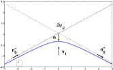
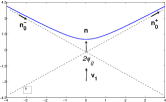
Figure 2: The relationship between the vectors in Eq.(3) a) an attractive force field and b) repulsive force field.

What we now argue is that the two cases are not symmetric. That is the kinetic energy loss (gain) in the approaching case is larger than the gain (loss) in the receding case for an(a) attractive (repulsive) potential. From Figs. (2a-b) we see that $\left|\mathbf{n}\right|=\textrm{2cos}\psi_{g}$. In the attractive case (Fig. 2a), if $m_{1}$ moves towards $m_{2}$ the angle between the asymptotes, $2\psi_{g}$, is smaller than it would be if $m_{1}$ moved away as the minimum distance is smaller. Therefore, $n=2\cos\psi_{g}$ is larger in the approaching case. For very high speed encounters, $\mathbf{\left|v_{2}\right|}\gg\mathbf{\left|v_{1}\right|}$, we can approximate $v$ to be the same in the two cases (Figs. 2 a and b), therefore Eq.(3) becomes:

$$\Delta E=\mu V\mathbf{V_{g}.}\mathbf{n\simeq\left\{\begin{array}[]{c}\mathit{-2\mu Vv_{1}}\left|\textrm{cos}\psi_{g}^{a}\right|\\ \hphantom{-}\mathit{2\mu Vv_{1}}\left|\textrm{cos}\psi_{g}^{r}\right|\end{array}\right.},$$ (4)

with $\left|\textrm{cos}\psi_{g}^{a}\right|>\left|\textrm{cos}\psi_{g}^{r}\right|$ (see following Eq.(10)).

Analytical Derivation- The heuristic arguments above apply to general central forces. For a two-body scattering based on laws of conservation of linear momentum and energy applicable to any law of interaction one can show Gryzinski1965_I ; Gryzinski1965_II

Figure 3: Initial configuration.

$$\Delta E = 2a\sin\psi_{g}\cos\psi_{g}\cos\Theta-b\cos^{2}\psi_{g}$$ (5)

$$a \equiv \mu v_{1}v_{2}\sin\theta,$$

$$b \equiv K_{12}\left[m_{2}v_{2}^{2}-m_{1}v_{1}^{2}+\left(m_{1}-m_{2}\right)v_{1}v_{2}\cos\theta\right],$$

$$K_{12} \equiv 2\left(m_{1}m_{2}\right)/\left(m_{1}+m_{2}\right)^{2}.$$

where $\Theta$ is the angle between the orbital and fundamental planes. The orbital plane is the plane perpendicular to the angular momentum vector and the fundamental plane contains $\mathbf{v_{1}}$ and $\mathbf{v_{2}}$. Eq.(5) is general and the law of interaction only enters through $\psi_{g}$.

What is needed is the full formulation of the scattering in the lab frame. For any given encounter, let us set up a coordinate system with the $\boldsymbol{\hat{z}}$ pointing in the direction of $\mathbf{v_{2}}$ and put $m_{1}$ at its origin as shown in Fig. 3. The initial state of $m_{2}$ is $\boldsymbol{r_{2}}=\left(x_{0},y_{0},-z_{0}\right)$ and $\mathbf{v_{2}}=\left(0,0,v_{2}\right)$ where we explicitly took $z_{0}>0$. The initial state of $m_{1}$ is $\boldsymbol{r_{1}}=\boldsymbol{0}$ and $\mathbf{v_{1}}=v_{1}\left(\sin\theta\cos\varphi,\sin\theta\sin\varphi,\cos\theta\right)$; consequently $V=\left\{v_{1}^{2}+v_{2}^{2}-2v_{1}v_{2}\cos\theta\right\}^{1/2}.$ The impact parameter $D$ is the minimum distance between the masses in the absence of interaction ($\alpha=0$). Both $D$ and $\Theta$ are functions of the relative states of the two masses SM ,

$$D = \left\{D_{0}^{2}-\frac{v_{1}\sin\theta}{V^{2}}\left[\frac{v_{1}}{2}\sin\theta\left(D_{0}^{2}-2z_{0}^{2}+\left(x_{0}^{2}-y_{0}^{2}\right)\cos 2\varphi+2x_{0}y_{0}\sin 2\varphi\right)+2v_{2}z_{0}\left(1-\frac{v_{1}}{v_{2}}\cos\theta\right)r_{0}\left(\varphi\right)\right]\right\}^{1/2},$$ (6)

$$\cos\Theta = \frac{r_{0}\left(\varphi\right)\left(v_{2}-v_{1}\cos\theta\right)-v_{1}z_{0}\sin\theta}{B},$$ (7)

$$B \equiv \left\{\left[v_{2}x_{0}-v_{1}\left(x_{0}\cos\theta+z_{0}\sin\theta\cos\varphi\right)\right]^{2}+v_{1}^{2}\sin^{2}\theta\left(-x_{0}\sin\varphi+y_{0}\cos\varphi\right)^{2}\right.$$

$$+ \left.\left[y_{0}\left(v_{2}-v_{1}\cos\theta\right)-v_{1}z_{0}\sin\theta\sin\varphi\right]^{2}\right\}^{1/2}.$$

where $D_{0}^{2}\equiv x_{0}^{2}+y_{0}^{2}$ and $r_{0}\left(\varphi\right)\equiv x_{0}\cos\varphi+y_{0}\sin\varphi$. From now on we confine to gravitational and Coulomb interactions goldstein . The strength of interaction, $\alpha$, for gravitational and Coulomb interactions are $Gm_{1}m_{2}$ and $\frac{q_{1}q_{2}}{4\pi\varepsilon_{0}}$ respectively and $\cos\psi_{g}=\frac{\alpha}{\mu V^{2}D}/\sqrt{1+\left(\frac{\alpha}{\mu V^{2}D}\right)^{2}}.$

The orbital and fundamental planes coincide for $y_{0}=0$, $\theta=\frac{\pi}{2}$ and $\varphi=0,\pi$. The special cases are: $\cos\Theta=1$ for $\varphi=0$ (approach) and $\cos\Theta=-1$ for $\varphi=\pi$ (recede). Ignoring terms of $\mathcal{O}\left(\frac{v_{1}}{v_{2}}\right)^{2}$ and higher, we find

$$\Delta E_{approach} = \frac{2\alpha}{D_{0}}\frac{v_{1}}{v_{2}}+\mathcal{O}\left(\frac{v_{1}}{v_{2}}\right)^{2},$$ (9)

$$\Delta E_{recede} = -\frac{2\alpha}{D_{0}}\frac{v_{1}}{v_{2}}+\mathcal{O}\left(\frac{v_{1}}{v_{2}}\right)^{2}.$$ (10)

Further, we find $\cos\psi_{g}^{a}=\frac{\alpha}{\mu D_{0}v_{2}^{2}}\left\{1+\left(\frac{v_{1}}{v_{2}}\right)\left[\frac{z_{0}}{D_{0}}\left(\frac{x_{0}}{D_{0}}\right)\right]\right\}$ and $\cos\psi_{g}^{r}=\frac{\alpha}{\mu D_{0}v_{2}^{2}}\left\{1-\left(\frac{v_{1}}{v_{2}}\right)\left[\frac{z_{0}}{D_{0}}\left(\frac{x_{0}}{D_{0}}\right)\right]\right\}$. Some conclusions can be drawn to first order in $\frac{v_{1}}{v_{2}}$:

1. For $\alpha<0$ the transverse collisions lead to small yet nonzero energy gain (loss) for the receding (approaching) collisions. For $\alpha>0$ the transverse collisions lead to small yet nonzero energy gain (loss) for the approaching (receding) collisions. This proves the heuristic arguments we gave earlier (depicted in Fig.1).

2. To investigate any asymmetry in $\Delta E$ (Fig. 1) one needs to go beyond $\mathcal{O}\left(\frac{v_{1}}{v_{2}}\right)$; see below.

3. We see that $\cos\psi_{g}^{r}<\cos\psi_{g}^{a}$ as argued above in and following Eq.(4).

We now calculate the ensemble average $\langle\Delta E\rangle_{\mathbf{\mathbf{v}_{1}}}$, where the subscript indicates the random variable with respect to which we average. It is useful to call $m_{2}$ the test particle undergoing small angle scattering through many collisions with field particles of mass $m_{1}$. Let $f\left(\theta,\varphi\right)d\theta d\varphi$ denote the probability that the velocity vector of a field particle has direction determined by angles $\theta$ and $\varphi$. For isotropically moving field particles $f\left(\theta,\varphi\right)=\frac{1}{2}\sin\theta\left(\frac{1}{2\pi}\right)$. Calculating $\Delta E$ as given by Eq.(5) and using Eqs.(6,7) and ignoring term of order $\mathcal{O}\left(\frac{v_{1}}{v_{2}}\right)^{3}$ and higher SM , we find $\langle\Delta E\rangle_{\theta,\varphi}\approx\frac{2}{3}\frac{\alpha}{D_{0}}\frac{z_{0}}{D_{0}}\left(\frac{v_{1}}{v_{2}}\right)^{2}+\mathcal{O}\left(\frac{v_{1}}{v_{2}}\right)^{3}$ .

It is found under rather general conditions that the speed of the field particles is Gaussian distributed $\frac{4j^{3}}{\sqrt{\pi}}e^{-j^{2}v_{1}^{2}}v_{1}^{2}dv_{1},$ where $j$ is related to the variance $\sigma$ by $j^{2}\equiv\frac{1}{\sqrt{2}\sigma^{2}}$ (chandra4, , Eq: 2.353). The integration with respect to $\rho\left(v_{1},\theta,\varphi\right)=\frac{j^{3}}{\pi^{3/2}}\sin\theta e^{-j^{2}v_{1}^{2}}v_{1}^{2}dv_{1}d\theta d\varphi$ gives the ensemble average,

$$\langle\Delta E\rangle_{\mathbf{\mathbf{v}_{1}}}=\frac{2\alpha}{D_{0}j^{2}v_{2}^{2}}\frac{z_{0}}{D_{0}}.$$ (11)

For a density of field particles $n$, adopting a cylindrical coordinate system in which the radius is $D_{0}$ and $\phi$ is the azimuthal angle, the number of field particles passing $m_{2}$ per unit time is $n\int d^{3}x/dt=n\left(\frac{dz}{dt}\right)\int dA$, which to leading order is $nv_{2}\int d\phi\int D_{0}dD_{0}$. Performing the integral we find

$$nv_{2}\int d\phi\int D_{0}dD_{0}\langle\Delta E\rangle_{\mathbf{\mathbf{v}_{1}}}=\frac{4\pi n\alpha z_{0}}{j^{2}v_{2}}\int\frac{dD_{0}}{D_{0}}$$

The integral diverges for $D_{0}\rightarrow\infty$; this is natural as the force is long range and by definition very distant encounters need to be taken into account. It also diverges for $D_{0}\rightarrow 0$, which violates the distant encounter assumptions $\frac{\alpha}{\mu DV^{2}}\ll 1$. However, in a given problem, there is a natural $D_{min}$ that ensures small angle scattering and a $D_{max}$, depending on the density of field particles. Further a factor of $2$ or $3$ error in choosing $D_{max}/D_{min}$ does not affect the calculation of relaxation times by much Divergent_Integral .

A typical time scale between collisions is $\delta t\sim 2z_{0}/v_{2}\sim n^{-1/3}/v_{2}$. The statistical change in energy of $m_{2}$ after $N$ encounters, denoted by $\langle\Delta E\rangle$ is $\frac{4\pi n\alpha z_{0}}{j^{2}v_{2}}\ln\left(\frac{D_{max}}{D_{min}}\right)N\delta t$ giving the desired result

$$\langle\Delta E\rangle\approx\frac{2\pi\alpha Nn^{1/3}}{j^{2}v_{2}^{2}}\ln\left(\frac{D_{max}}{D_{min}}\right).$$ (12)

Note that attractive interactions, i.e., $\alpha<0$, yield an average loss and $\alpha>0$ an average gain.

Statistical Context- A phenomena worth considering is dynamical friction chandra1 ; chandra2 . Dynamical friction, however, is like Brownian motion einstein as a big mass enters a medium of many smaller particles and slows down as a result. But it is distinct from Brownian motion as the interactions are long ranged. It is found that in dynamical friction “only stars with velocities less than the one under consideration contribute to the effect” chandra3 and (chandra4, , p. 299).

The main requirement here is that the test particle scatters from the time-dependent field of, in comparison massive, particles that are moving randomly and slowly in space, through a series of small-angle scatterings.

At first sight this effect seems to violate the equipartition of energy because a low energy particle “heats up” the medium of much larger particles that have higher energies. We are working with a non-equilibrium process in an open system. In attractive potentials the small particle starts from non-equilibrium initial conditions and through a series of scatterings it statistically loses energy till a final scattering where the energy in the center of mass is negative. There on the small particle would have a bounded orbit about that final scatterer. This corresponds to the breakdown of small angle scattering assumption we have made. In plasma physics this is known as shielding and in astrophysics it corresponds to capturing of a comet by a center of force. In repulsive potentials the energy of the small particle grows till the relativistic effects become significant and the transfer of energy between the small particle and the scatterers becomes of order unity with respect to the initial energy (LandauLifshitzFields, , section 13). Hence the effect is not an equilibration process and is applicable to systems where the assumptions of small angle scattering, as well as, $m_{1}\ll m_{2}$, $v_{1}\gg v_{2}$ but nevertheless $m_{1}v_{1}^{2}\ll m_{2}v_{2}^{2}$ hold. The small angle scattering assumption is bound to break on time scales comparable to the relaxation time to equilibrium.

If we relax the assumption $m_{1}\gg m_{2}$ and let $m_{1}$ be comparable to $m_{2}$, then for small angle scatterings and $v_{2}\gg v_{1}$ one finds that $\langle\Delta E\rangle<0$ regardless of the sign of $\alpha$ as expected ((SM, , Section 3.1)).

It would be interesting to analyze the effect of micro-dynamics of the structure in the universe on the frequency shift of photons coming from distant sources. We expect a small loss of energy for photons that undergo dynamical weak lensing weinberg ; tyson . We hope this work helps better understanding of rapid structure formation peebles , high energy cosmic rays cosmicRay and redshift problem Reyes .

Supplementary Material. Two-Particle Collisions: The Laboratory Frame Formulation

Let us consider an encounter between two particles of masses $m_{1}$ and $m_{2}$. If the initial conditions are specified, the dynamics in principle is fully determined. To fully specify the state at any time one needs $12$ parameters; $3$ positions and $3$ momenta per particle. A system of $n$ interacting particles that are isolated otherwise have conservation of energy, linear and angular momentum intact regardless of the particular laws of interaction among the constituents. This applies to the two body problem ($n=2$) as well and provides us with $7$ constraints, $1$ energy $3$ linear and $3$ angular momenta. Therefore there are $5$ other degrees of freedom that depend on the geometry of the encounter and the law of interaction.

Figure 4: Initial and final velocities with respect to the laboratory system. $\boldsymbol{v_{1}}$ and $\boldsymbol{v_{2}}$ define the fundamental plane.

Below we denote vectors in boldface (e.g., $\boldsymbol{v_{1}}$ is a vector with magnitude $v_{1}$). Let the velocities before the collision be $\boldsymbol{v_{1}}$ and $\boldsymbol{v_{2}}$ and after $\boldsymbol{v_{1}^{\prime}}$ and $\boldsymbol{v_{2}^{\prime}}$. We take the $z$ axis of the laboratory system to coincide with the initial direction of particle $2$, which we call the test particle. As a result of interaction with particle $1$, which we call the field particle, the velocity of particle $2$ changes in magnitude and direction. We denote the change in the energy of particle $2$ by $\Delta E$, the direction of velocity after the scattering by $\vartheta$ and $\phi$ (Gryzinski1965_I, , Figure 1). Similarly we assign $\Delta\tilde{E}$, $\tilde{\vartheta}$ and $\tilde{\phi}$ for the field particle. It is clear that the result of collision depends on the laws of interaction as well as the geometry of encounter. To describe the geometry of the encounter, we need four geometrical quantities (one linear quantity and three angular ones (Gryzinski1965_I, , Figure 2))

1. the collision impact parameter $D$

2. the angle $\theta$ which is the angle between $\boldsymbol{v_{1}}$ and $\boldsymbol{v_{2}}$; the plane containing these two vectors is called the fundamental plane

3. the angle $\Theta$, which is the angle formed by the segment $D$ with the fundamental plane. Equivalently this is the angle between the orbital plane and the fundamental plane. The orbital plane is the plane perpendicular to the angular momentum vector and contains the relative velocity before and after the collision.

4. the angle $\varphi$, which is the angle describing the position of the fundamental plane with respect to rotation about the $z$ axis.

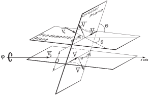
Figure 5: Space diagram of the encounter. The orbital plane contains $\boldsymbol{V}$ and $\boldsymbol{V^{\prime}}$. The law of interaction is completely encoded in $\psi_{g}$.

The range of these parameters are (Gryzinski1965_I, , Figure 2)

$$0 \leq D\leq \infty,$$

$$0 \leq\theta\leq \pi,$$

$$0 \leq\Theta\leq 2\pi,$$

$$0 \leq\varphi\leq 2\pi.$$

Now we shall derive the dependence of $\Delta E$, $\vartheta$,$\phi$ and $\Delta\tilde{E}$, $\tilde{\vartheta}$ ,$\tilde{\phi}$ in term of the geometrical quantities. The fifth parameter, which encodes the dependence on the law of interaction is $\psi_{g}$– the scattering angle in the center of mass frame.

.1 Law of interaction and $\psi_{g}$

The dependence on the interaction law only enters through the trigonometric functions of the angle $\psi_{g}$, i.e., the angle describing the scattering of the reduced mass $\mu$ in the center of mass system. Therefore, for a unified formulation that applies to repulsive and attractive force laws given by the potential $U\left(r\right)=\frac{\alpha}{r^{k}}$ where

$$\alpha < 0\mbox{ }:\quad\mbox{attractive}$$

$$\alpha > 0\mbox{ }:\quad\mbox{repulsive}$$

it is necessary that the sign of the interaction enters the formulas derived for $\psi_{g}$. The importance of this is especially pronounced when considering collision statistics. In calculating a scalar quantity $\psi_{g}$ and ignoring the origin with respect to which it extends ignores the sign of the interaction (see Figure 6).

Figure 6: Scattering and deflection angles shown in $\psi_{g}$ and $\chi$ respectively.

The scattering for $k=1$ corresponds to hyperbolic trajectories in the center of mass frame. For the sake of concreteness let us consider a Coulomb scattering where we have a force field with charge $+Ze$ pinned down, shown as a black center in the Figure 6. Take that be a focal point of the hyperbola which has two branches one shown in black and the other in grey dashed curve. We put an arrow head to emphasize the temporal order of the points on each branch. The solid black branch corresponds to a positive particle, say a positron $+e$, coming from $-\infty$ (i.e., left) and scattering off. The grey dashed branch corresponds to an electron coming from $+\infty$ (i.e., right). The minimum distances from the center of the force in both cases lie on the same line, albeit the magnitudes are different ($-e$ gets closer to the center of the force).

The black branch describes the scattering in a repulsive force field. How does the scattering look if we consider an electron coming from $-\infty$? This corresponds to the reflection of the dashed grey branch, shown as a solid grey, about the vertical axis piercing the center of the force (the vertical axis is shown by a thin dashed line). The geometry makes it clear that $\psi_{g}$ for this case is greater than $\frac{\pi}{2}$, whereas it is less than $\frac{\pi}{2}$ for the repulsive force field and it is exactly $\frac{\pi}{2}$ when there is no interaction. The calculation of the angle correspondingly gives a negative value for $\cos\psi_{g}$ in an attractive force field and a positive value in a repulsive force field.

We are concerned with interactions that are central, they depend only on the distance between the particles, then the relation describing the angle $\psi_{g}$ is relatively simple

$$\psi_{g}=\intop_{r_{min}}^{\infty}\frac{\left(D/r^{2}\right)dr}{\left\{1-\frac{2U\left(r\right)}{\mu V^{2}}-\left(D/r\right)^{2}\right\}^{1/2}},$$ (13)

where $\mu=\frac{m_{1}m_{2}}{m_{1}+m_{2}}$, $V$and $D$ have the same meaning as above and $U\left(r\right)$ is the potential function of the two particles and $r_{min}$ is the distance of closest approach of $\mu$ to the center of force determined by the turning point at which $\dot{r}=0$. Let $\rho=\frac{D}{r}$, the potential becomes $\tilde{U}\left(\rho\right)=\frac{\alpha\rho^{k}}{D^{k}}$ and the scattering angle

$$\psi_{g}=\intop_{0}^{\rho_{max}}\frac{d\rho}{\left\{1-\frac{2\alpha}{\mu V^{2}}\left(\frac{\rho}{D}\right)^{k}-\rho^{2}\right\}^{1/2}},$$ (14)

where $\rho_{max}$ is the positive root of the quantity in the denominator. In scattering problems energy in the center of mass $E>0$ hence $\frac{\mu}{2}V^{2}+U>0$ which implies $-\frac{2U}{\mu V^{2}}<1.$ For $U\left(r\right)=\frac{\alpha}{r^{k}}$ this becomes $-\frac{2\alpha}{\mu V^{2}r^{k}}<1$. The inequality is trivially satisfied for $\alpha>0$ and for attractive potentials implies $0\leq\frac{2\left|\alpha\right|}{\mu V^{2}r^{k}}<1$ and $2\left|\alpha\right|<\mu V^{2}r^{k}$. Eq. 14 for $k=1$ is an elementary integral of form

$$\int\frac{dx}{\sqrt{a+bx+cx^{2}}} = \frac{1}{\sqrt{-c}}\cos^{-1}\left(-\frac{b+2cx}{\sqrt{\lambda}}\right)$$

$$\lambda \equiv b^{2}-4ac,$$

substituting we find

$$\psi_{g} = \cos^{-1}\frac{\epsilon+\rho}{\sqrt{1+\epsilon^{2}}}$$

$$\epsilon \equiv \frac{\alpha}{\mu V^{2}D}$$

Further

$$\rho_{max}=-\epsilon+\sqrt{1+\epsilon^{2}}.$$

Performing the integral we get

$$\cos\psi_{g} = \frac{\epsilon}{\sqrt{1+\epsilon^{2}}}=\frac{\frac{\alpha}{\mu V^{2}D}}{\sqrt{1+\left(\frac{\alpha}{\mu V^{2}D}\right)^{2}}}$$ (15)

$$\sin\psi_{g} = \frac{1}{\sqrt{1+\epsilon^{2}}}=\frac{1}{\sqrt{1+\left(\frac{\alpha}{\mu V^{2}D}\right)^{2}}}$$ (16)

Below we mainly deal with the case of $k=1$. Though it is irrelevant for most of what follows, as an aside, for $k=2$, the integration yields

$$\psi_{g}=\frac{\pi}{2}\frac{1}{\left\{1+\left(\frac{2\alpha}{\mu V^{2}D^{2}}\right)\right\}^{1/2}}.$$ (17)

Moreover, we mention that in the case of a collision of two impenetrable spheres of radii $R_{1}$ and $R_{2}$, Eq. 14 gives

$$\sin\psi_{g} = 2D/\left(R_{1}+R_{2}\right),$$

$$\cos\psi_{g} = \left\{1-\left[2D/\left(R_{1}+R_{2}\right)\right]^{2}\right\}^{1/2}.$$

Dynamics of a Two-Particle Encounter

The relations we derive in this section are in the most general form based on laws of conservation of linear momentum and energy applicable to any law of interaction. By momentum conservation, the velocity of the center of mass $\boldsymbol{V_{g}}$ is a constant

$$m_{1}\boldsymbol{v_{1}}+m_{2}\boldsymbol{v_{2}}=m_{1}\boldsymbol{v_{1}^{\prime}}+m_{2}\boldsymbol{v_{2}^{\prime}}\equiv\left(m_{1}+m_{2}\right)\boldsymbol{V_{g}}.$$

Hence we can write, denoting $M_{1}=m_{1}/\left(m_{1}+m_{2}\right)$ and $M_{2}=m_{2}/\left(m_{1}+m_{2}\right)$

$$V_{g}^{2}=M_{1}^{2}v_{1}^{2}+M_{2}^{2}v_{2}^{2}+2M_{1}M_{2}v_{1}v_{2}\cos\theta.$$ (18)

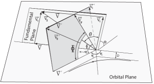
Figure 7: Velocities for the two particle collision.

Let $\boldsymbol{V}\equiv\boldsymbol{v_{2}-v_{1}}$ and $\boldsymbol{V}^{\prime}\equiv\boldsymbol{v_{2}^{\prime}-v_{1}^{\prime}}$ which using the above relations we can write

$$\begin{array}[]{ccc}\boldsymbol{v_{1}}=\boldsymbol{V_{g}}-M_{2}\boldsymbol{V},&&\boldsymbol{v_{1}^{\prime}}=\boldsymbol{V_{g}}-M_{2}\boldsymbol{V^{\prime};}\\ \boldsymbol{v_{2}}=\boldsymbol{V_{g}}+M_{1}\boldsymbol{V},&&\boldsymbol{v_{2}^{\prime}}=\boldsymbol{V_{g}}+M_{2}\boldsymbol{V^{\prime}.}\end{array}$$ (19)

Since the scattering is elastic, the total kinetic energy is conserved

$$\frac{1}{2}m_{1}v_{1}^{2}+\frac{1}{2}m_{2}v_{2}^{2}=\frac{1}{2}m_{1}v_{1}^{{}^{\prime}}\mbox{}^{2}+\frac{1}{2}m_{2}v^{\prime}_{2}\mbox{}^{2};$$

it is easy to see that $V=V^{\prime}$, namely the relative velocity only changes in direction and not magnitude. The dynamical effect of encounter is therefore known when the change in the direction of $V$ is determined; hence the importance of the scattering angle.

.2 Calculation of $\Delta E$

By definition $\Delta E=\frac{1}{2}m_{2}v_{2}^{{}^{\prime}}\mbox{}^{2}-\frac{1}{2}m_{2}v_{2}^{2}$ and is positive when the test particle gains energy in collision and is negative when it loses energy. Squaring the quantities in Eq. 19, we have

$$v_{2}^{2} = V_{g}^{2}+2M_{1}V_{g}V\cos\Phi+M_{1}^{2}V^{2},$$ (20)

$$v_{1}^{2} = V_{g}^{2}-2M_{2}V_{g}V\cos\Phi+M_{2}^{2}V^{2},$$ (21)

where $\Phi$ is the angle between $\boldsymbol{V_{g}}$ and $\boldsymbol{V}$. Similarly after the encounter we have

$$v^{\prime}_{2}\mbox{}^{2}=V_{g}^{2}+2M_{1}V_{g}V^{\prime}\cos\Phi^{\prime}+M_{1}^{2}V^{\prime}\mbox{}^{2}$$

where $\Phi^{\prime}$ is the angle between $\boldsymbol{V_{g}}$ and $\boldsymbol{V^{\prime}}$. Since $V=V^{\prime}$

$$\Delta E = \frac{1}{2}m_{2}\left(v^{\prime}_{2}\mbox{}^{2}-v_{2}^{2}\right)$$ (22)

$$= \frac{m_{1}m_{2}}{m_{1}+m_{2}}V_{g}V\left(\cos\Phi^{\prime}-\cos\Phi\right).$$

Solving 21 and using 18 and 19 for $\cos\Phi$ and using geometry to infer $\cos\Phi^{\prime}$ we obtain

$$\cos\Phi = \frac{m_{2}v_{2}^{2}-m_{1}v_{1}^{2}+\left(m_{1}-m_{2}\right)v_{1}v_{2}\cos\theta}{\left(m_{1}+m_{2}\right)V_{g}V}$$

$$\cos\Phi^{\prime} = \cos\Phi\cos\left(\pi-2\psi_{g}\right)+\sin\Phi\sin\left(\pi-2\psi_{g}\right)\cos\Theta.$$

Comment: Let $\mbox{sgn}\alpha$ denote the sign of the interaction; i.e., $\mbox{sgn}\alpha=+1$ for repulsive and $\mbox{sgn}\alpha=-1$ for attractive interactions. Note that $\sin\left(\pi-2\psi_{g}\right)=\mbox{sgn}\alpha\sin\left(\left|\pi-2\psi_{g}\right|\right)$ .

Using these

$$\Delta E=-\frac{2m_{1}m_{2}}{m_{1}+m_{2}}V_{g}V\cos^{2}\psi_{g}\left(\cos\Phi-\sin\Phi\cos\Theta\tan\psi_{g}\right).$$

This can be written in its final form

$$\Delta E=2a\sin\psi_{g}\cos\psi_{g}\cos\Theta-b\cos^{2}\psi_{g},$$ (23)

where

$$a = \mu v_{1}v_{2}\sin\theta$$

$$b = K_{12}\left[\frac{1}{2}m_{2}v_{2}^{2}-\frac{1}{2}m_{1}v_{1}^{2}+\frac{1}{2}\left(m_{1}-m_{2}\right)v_{1}v_{2}\cos\theta\right],$$

and

$$\mu \equiv \left(m_{1}m_{2}\right)/\left(m_{1}+m_{2}\right),$$

$$K_{12} \equiv 4\left(m_{1}m_{2}\right)/\left(m_{1}+m_{2}\right)^{2}.$$

Below we will use this form of the equations.

Alternatively, one can expand $\sin\theta$ and $\cos\theta$ in terms of relative velocity $V$, and write $a$ and $b$ in the form

$$a = \frac{\mu}{2}\left[-V^{4}+2V^{2}\left(v_{1}^{2}+v_{2}^{2}\right)-\left(v_{2}^{2}-v_{1}^{2}\right)^{2}\right]^{1/2}$$

$$b = \mu\left(v_{2}^{2}-v_{1}^{2}+\frac{m_{2}-m_{2}}{m_{2}+m_{1}}V^{2}\right).$$

Similarly equations for $\Delta\tilde{E}$,$\vartheta$,$\phi$, $\tilde{\vartheta}$ ,$\tilde{\phi}$ can be obtained Gryzinski1965_I .

I Geometry and Dynamics Entirely in The Laboratory System

I.1 $\boldsymbol{V}$, $D$ and $\Theta$ in laboratory system

We distinguish between geometrical coordinates and the dynamical coordinates. By geometrical coordinates we have in mind the configuration of the system when the two particles do not interact and with dynamical coordinates we have in mind the coordinates in the presence of the force between the particles. In order to express the impact parameter $D$ and relative velocity $\boldsymbol{V}$ entirely in the laboratory frame, we work with the geometrical coordinates.

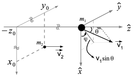
Figure 8: The initial configuration

For any given encounter, let us set up a coordinate system with the $\boldsymbol{\hat{z}}$ pointing in the direction of $\boldsymbol{v_{2}}$ and put the field particle at its origin. The relative position and velocity are readily expressed in the lab frame respectively by $\boldsymbol{r}=\boldsymbol{r}_{2}-\boldsymbol{r}_{1}=x_{0}\hat{\boldsymbol{x}}+y_{0}\hat{\boldsymbol{y}}-z_{0}\hat{\boldsymbol{z}}$ and $\boldsymbol{V}=\left(v_{1}\sin\theta\cos\varphi\right)\hat{\boldsymbol{x}}+\left(v_{1}\sin\theta\sin\varphi\right)\hat{\boldsymbol{y}}+\left(v_{1}\cos\theta-v_{2}\right)\hat{\boldsymbol{z}}$ and $V=\left\{v_{1}^{2}+v_{2}^{2}-2v_{1}v_{2}\cos\theta\right\}^{1/2}.$ The configuration is shown in Figure 8.

The impact parameter is the distance of closest approach and is obtained by considering the parametric equations of the lines that each particle traces and finding the minimum distance between those lines. Let the line traced by the first particle be denoted by $l_{1}$ and the line traced by the second particle $l_{2}$. It is necessary to provide some information regarding the initial configuration by providing the coordinates of the second particle (first particle being at the origin in $t=0$). Let the second particle have coordinates $\left(x_{0},y_{0},-z_{0}\right)$, where we take $z_{0}>0$. Then any point on $l_{1}$ denoted by $P_{1}$ and any point on $l_{2}$ denoted by $P_{2}$ at time $t$ is

$$P_{1}\left(t\right) = v_{1}t\left(\sin\theta\cos\varphi,\sin\theta\sin\varphi,\cos\theta\right)$$

$$P_{2}\left(t\right) = \left(x_{0},y_{o},-z_{0}+v_{2}t\right).$$

The impact parameter corresponds to the distance between the points at a time denoted by $t_{*}$ when $\left|P_{2}\left(t\right)-P_{1}\left(t\right)\right|$ is minimized. That time $t_{*}$ is found by $\frac{d}{dt}\left[P_{2}\left(t\right)-P_{1}\left(t\right)\right]^{2}=0$, where $P_{2}\left(t\right)-P_{1}\left(t\right)=\left(x_{0}-v_{1}t\sin\theta\cos\varphi,y_{0}-v_{1}t\sin\theta\sin\varphi,-z_{0}+v_{2}t-v_{1}t\cos\theta\right)$

$$\left[P_{2}\left(t\right)-P_{1}\left(t\right)\right]^{2} = \left\{t^{2}\left(v_{1}^{2}+v_{2}^{2}-2v_{1}v_{2}\cos\theta\right)+x_{0}^{2}+y_{0}^{2}+z_{0}^{2}\right.$$

$$\left.-2t\left[v_{1}y_{0}\sin\theta\cos\varphi+v_{1}y_{0}\sin\theta\sin\varphi+z_{0}\left(v_{2}-v_{1}\cos\theta\right)\right]\right\}$$

$$\frac{d}{dt}\left[P_{2}\left(t_{*}\right)-P_{1}\left(t_{*}\right)\right]^{2}=0 \implies t_{*}=\frac{v_{1}\sin\theta\left(x_{0}\cos\varphi+y_{0}\sin\varphi\right)+z_{0}\left(v_{2}-v_{1}\cos\theta\right)}{v_{1}^{2}+v_{2}^{2}-2v_{1}v_{2}\cos\theta}.$$

Therefore,

$$D \equiv \left|P_{2}\left(t_{*}\right)-P_{1}\left(t_{*}\right)\right|$$

$$= \left\{x_{0}^{2}+y_{0}^{2}-\frac{v_{1}\sin\theta}{V^{2}}\left[\frac{v_{1}}{2}\sin\theta\left(x_{0}^{2}+y_{0}^{2}-2z_{0}^{2}+\left(x_{0}^{2}-y_{0}^{2}\right)\cos 2\varphi+2x_{0}y_{0}\sin 2\varphi\right)\right.\right.$$

$$\left.\left.+2v_{2}z_{0}\left(1-\frac{v_{1}}{v_{2}}\cos\theta\right)\left(x_{0}\cos\varphi+y_{0}\sin\varphi\right)\right]\right\}^{1/2}$$

$\Theta$ is the angle between the fundamental and orbital planes and is defined by $\cos\Theta=\boldsymbol{\hat{n}_{orb}}\cdot\boldsymbol{\hat{n}_{F}}$, where $\boldsymbol{\hat{n}_{orb}}=\frac{\boldsymbol{r}\times\boldsymbol{V}}{\left|\boldsymbol{r\times}\boldsymbol{V}\right|}$ and $\boldsymbol{\hat{n}_{F}}\equiv\frac{\boldsymbol{v_{1}\times}\boldsymbol{v_{2}}}{v_{1}v_{2}\sin\theta}$ are the unit vectors perpendicular to the orbital and the fundamental planes respectively

$$\boldsymbol{\hat{n}_{F}} = \left(\sin\varphi,-\cos\varphi,0\right),$$

$$\boldsymbol{\hat{n}_{orb}} = \frac{1}{\left|\boldsymbol{r\times}\boldsymbol{V}\right|}\left(n_{orb}^{x},n_{orb}^{y},n_{orb}^{z}\right),$$

$$n_{orb}^{x} \equiv y_{0}\left(v_{2}-v_{1}\cos\theta\right)-v_{1}z_{0}\sin\theta\sin\varphi,$$

$$n_{orb}^{y} \equiv -v_{2}x_{0}+v_{1}\left(x_{0}\cos\theta+z_{0}\sin\theta\cos\varphi\right),$$

$$n_{orb}^{z} \equiv v_{1}\sin\theta\left(y_{0}\cos\varphi-x_{0}\sin\varphi\right),$$

which gives

$$\cos\Theta = \frac{\left(x_{0}\cos\varphi+y_{0}\sin\varphi\right)\left(v_{2}-v_{1}\cos\theta\right)-v_{1}z_{0}\sin\theta}{B}$$

$$B \equiv \left\{\left[v_{2}x_{0}-v_{1}\left(x_{0}\cos\theta+z_{0}\sin\theta\cos\varphi\right)\right]^{2}\right.$$

$$+ v_{1}^{2}\sin^{2}\theta\left(-x_{0}\sin\varphi+y_{0}\cos\varphi\right)^{2}$$

$$+ \left.\left[y_{0}\left(v_{2}-v_{1}\cos\theta\right)-v_{1}z_{0}\sin\theta\sin\varphi\right]^{2}\right\}^{1/2}.$$

The orbital and fundamental planes coincide for $y_{0}=0$, $\theta=\frac{\pi}{2}$ and $\varphi=0,\pi$. We see that in these special cases taking $y_{0}=0$ and $\theta=\frac{\pi}{2}$

$$\cos\Theta = \frac{x_{0}v_{2}-v_{1}z_{0}}{\sqrt{\left(v_{2}x_{0}-v_{1}z_{0}\right)^{2}}}=1\qquad\varphi=0$$ (25)

$$\cos\Theta = \frac{-x_{0}v_{2}-v_{1}z_{0}}{\sqrt{\left(v_{2}x_{0}+v_{1}z_{0}\right)^{2}}}=-1\qquad\varphi=\pi.$$ (26)

I.2 Effective Collision Times

The discussions so far refer to ideal scattering processes where the particles start infinitely apart and go to infinity after the collision takes place. The scattering angle $\psi_{g}$ is the angle between the two asymptotes. In real collisions, as the ones being considered here, the test particle scatters from many field particles that are far yet at finite distances from one another. Therefore, $\psi_{g}$ over-estimates the actual scattering angle per collision. Since the entire effect of interaction is uniquely determined by $\psi_{g}$, we let define the collision time to be the time after which this angle attains a value close to the value it would have attained in infinite time. In the case of central forces under consideration Gryzinski (Gryzinski1965_I, , Section IV) divides the collisions to two types by defining a parameter $r_{0}$ to be the distance at which the potential energy of the two particles is equal to the relative kinetic energy. The collisions with an impact parameter $D<r_{0}$ are called the “close collisions” with $D>r_{0}$ are called “distant collisions”. The collision time for central forces with potential $U\left(r\right)=\frac{\alpha}{r^{k}}$ are shown to be Gryzinski1965_I

$$t_{coll}\approx 2\left[\left(r_{0}+D\right)/V\right]\left(2^{1/k}-1\right),$$

which for the Coulomb interaction $k=1$ becomes $t_{coll}\approx 2\left[\left(r_{0}+D\right)/V\right]$.

In addition, for a series of two-body scatterings to be a sensible approximation of the many-body phenomena the time of collision needs to be much shorter than the time it takes for the test or field particle to have an appreciable change in their velocities due to interaction with other particles or external fields.

I.3 Small Angle Scattering

So far the formulation has been exact. For potentials of type $\alpha/r^{k}$ a small angle scattering corresponds to $D\gg\frac{\alpha}{\mu V^{2}}$. We show this for $k=1,2$ and note that for $k>2$ the field strength decreases stronger with the distance and the same condition $D\gg\frac{\alpha}{\mu V^{2}}$ ought to suffice. This can be seen from Eqs. 15 - 17 which in this limit read

$$\sin\psi_{g} \underset{=}{\left(k=1\right)} \frac{1}{\left\{1+\left(\frac{\alpha}{\mu DV^{2}}\right)^{2}\right\}^{1/2}}\approx\left\{1-\frac{1}{2}\left(\frac{\alpha}{\mu DV^{2}}\right)^{2}\right\},$$

$$\cos\psi_{g} \underset{=}{\left(k=1\right)} \left(\frac{\alpha}{\mu DV^{2}}\right)\left\{1+\left(\frac{\alpha}{\mu DV^{2}}\right)^{2}\right\}^{-1/2}\approx\frac{\alpha}{\mu DV^{2}},$$

$$\psi_{g} \underset{=}{\left(k=2\right)} \frac{\pi}{2}\frac{1}{\left\{1+\left(\frac{2\alpha}{\mu V^{2}D^{2}}\right)\right\}^{1/2}}\approx\frac{\pi}{2}\left[1-\left(\frac{\alpha}{\mu D^{2}V^{2}}\right)\right].$$

Since $\Delta E$ depends on it, we approximate $\sin\psi_{g}\cos\psi_{g}\approx\frac{\alpha}{\mu DV^{2}}\left[1-\left(\frac{\alpha}{\mu DV^{2}}\right)^{2}\right].$ From now on we restrict ourselves to the important case of $k=1$.

Comment: There are two small parameters under consideration. 1. $\frac{\alpha}{\mu V^{2}}\ll D$ which allows us to approximate the dynamical quantities and 2. $\frac{v_{1}}{v_{2}}$ that we use for approximating the geometric quantities. We shall see that terms of order $\left(\frac{v_{1}}{v_{2}}\right)^{2}$ are necessary to keep to obtain the asymmetry we seek in the ensemble average $\langle\Delta E\rangle_{\boldsymbol{v_{1}}}$.

Below we keep to second order in $\frac{\alpha}{\mu DV^{2}}$.

II Statistics: Ensemble Average

What needs to be done for our purposes is to calculate the ensemble average $\langle\Delta E\rangle_{\boldsymbol{v_{1}}}$, where by the subscript we have in mind average with respect to random variable $\boldsymbol{v_{1}}$. To bring out the effect first let us fix the speed $v_{1}$ and let $f\left(\theta,\varphi\right)d\theta d\varphi$ denote the probability that the velocity vector of $m_{1}$ has direction determined by angles $\theta$ and $\varphi$. For isotropically moving field particles $f\left(\theta,\varphi\right)=\frac{1}{2}\sin\theta\left(\frac{1}{2\pi}\right)$. It is found under rather general conditions that the distribution function of the speed of the field stars is given by (chandra4, , Eq: 2.353)

$$N\left(v_{1}\right)dv_{1}=\frac{4j^{3}}{\sqrt{\pi}}Ne^{-j^{2}v_{1}^{2}}v_{1}^{2}dv_{1}.$$

The measure for the ensemble average then becomes

$$f\left(\theta,\varphi\right)N\left(v_{1}\right)dv_{1}d\theta d\varphi=\frac{Nj^{3}}{\pi^{3/2}}\sin\theta e^{-j^{2}v_{1}^{2}}v_{1}^{2}dv_{1}d\theta d\varphi$$ (27)

II.1 $v_{1}\ll v_{2}$ and small angle scattering and $m_{2}\sim m_{1}$

When the masses are comparable one expects that $m_{2}$ on average would impart energy to $m_{1}$. We include this case as a side calculation because of its simplicity and relevance for phenomena beyond the scope of this work. From above we have

$$\Delta E=2a\sin\psi_{g}\cos\psi_{g}\cos\Theta-b\cos^{2}\psi_{g},$$

where $\mu=\frac{m_{1}m_{2}}{m_{1}+m_{2}}$ and $K_{12}\equiv\frac{4\mu}{m_{1}+m_{2}}$

$$a = \mu v_{1}v_{2}\sin\theta$$

$$b = K_{12}\left[\frac{1}{2}m_{2}v_{2}^{2}-\frac{1}{2}m_{1}v_{1}^{2}+\frac{1}{2}\left(m_{1}-m_{2}\right)v_{1}v_{2}\cos\theta\right]$$

$$\frac{1}{4\pi}\int d\theta d\varphi\sin\theta\Delta E = \frac{1}{4\pi}\int d\theta d\varphi\sin\theta\left\{2a\sin\psi_{g}\cos\psi_{g}\cos\Theta\right\}$$

$$- \frac{1}{4\pi}\int d\theta d\varphi\sin\theta\left\{b\cos^{2}\psi_{g}\right\}$$

To zeroth order in $\frac{v_{1}}{v_{2}}$ we find $\sin\psi_{g}\approx\frac{\mu v_{2}^{2}D_{0}}{\sqrt{1+\frac{\left(\mu v_{2}^{2}D_{0}\right)^{2}}{\alpha}}}$ and $\cos\psi_{g}\approx\left\{1+\left(\frac{\mu v_{2}^{2}D_{0}}{\alpha}\right)^{2}\right\}^{-1/2}$. Consequently to zeroth order we find $2a\sin\psi_{g}\cos\psi_{g}\cos\Theta\approx 0$ and $b\cos^{2}\psi_{g}\approx\frac{2m_{1}\left(m_{2}v_{2}\alpha\right)^{2}}{\left(m_{1}m_{2}v_{2}^{2}D_{0}\right)^{2}+\left(m_{1}+m_{2}\right)^{2}\alpha^{2}}$, which readily gives us a first order effect

$$\langle\Delta E\rangle_{\theta,\varphi}=-\frac{2m_{1}\left(m_{2}v_{2}\alpha\right)^{2}}{\left(m_{1}m_{2}v_{2}^{2}D_{0}\right)^{2}+\left(m_{1}+m_{2}\right)^{2}\alpha^{2}}+\mathcal{O}\left(\frac{v_{1}}{v_{2}}\right).$$

Note that we did not make approximations using $m_{2}\ll m_{1}$. We see that regardless of the sign of the interaction, the condition $v_{1}\ll v_{2}$ implies that the fast particle on average must lose energy to the slower one.

II.2 Approximation of dynamical quantities via: $m_{2}\ll m_{1}$ , $v_{2}\gg v_{1}$ but $m_{1}v_{1}^{2}\gg m_{2}v_{2}^{2}$

The relation $D\gg\frac{\alpha}{\mu V^{2}}$ can be satisfied in various ways. We are interested in glazing collisions of $\boldsymbol{v_{2}}$ from $\boldsymbol{v_{1}}$ such that $v_{1}\ll v_{2}$ and $m_{2}\ll m_{1}$ but $m_{1}v_{1}^{2}\gg m_{2}v_{2}^{2}$. These conditions together imply $m_{1}v_{1}\gg m_{2}v_{2}$. The relative momenta are important for our purposes of calculating the ensemble average $\langle\Delta E\rangle_{\boldsymbol{v_{1}}}$, where by the subscript we have in mind average with respect to random variable $\boldsymbol{v_{1}}$. From above we have

$$\Delta E=2a\sin\psi_{g}\cos\psi_{g}\cos\Theta-b\cos^{2}\psi_{g},$$

which in the limit is specified by

$$a = \mu v_{1}v_{2}\sin\theta\approx m_{2}v_{1}v_{2}\sin\theta$$ (28)

$$b = K_{12}\left[\frac{1}{2}m_{2}v_{2}^{2}-\frac{1}{2}m_{1}v_{1}^{2}+\frac{1}{2}\left(m_{1}-m_{2}\right)v_{1}v_{2}\cos\theta\right]$$ (29)

$$\approx 2m_{2}v_{2}^{2}\left(\frac{v_{1}}{v_{2}}\right)\left(\cos\theta-\frac{v_{1}}{v_{2}}\right).$$

where $\mu=\frac{m_{1}m_{2}}{m_{1}+m_{2}}$ and $K_{12}\equiv\frac{4\mu}{m_{1}+m_{2}}$. In order to calculate $\Delta E$ we need to approximate the geometric quantities.

II.3 Approximation of geometrical quantities to first order in $\left(\frac{v_{1}}{v_{2}}\right)$

The condition $v_{1}\ll v_{2}$ is enough to allow approximations of the geometrical coordinates. The inertia of the particles and the strength of the interaction are irrelevant in calculation of the geometric coordinates.

Here to make appropriate approximations we assume $x_{0},y_{o},z_{0}$ are of the same order of magnitude (see Figure 8). We then calculate the ensemble average ignoring terms of $\mathcal{O}\left(\frac{v_{1}}{v_{2}}\right)^{2}$ and higher

$$V^{2} \approx v_{2}^{2}\left(1-\frac{2v_{1}}{v_{2}}\cos\theta\right)$$

$$v_{z} = v_{2}\left(1-\frac{v_{1}}{v_{2}}\cos\theta\right)$$

$$D \approx \left\{x_{0}^{2}+y_{0}^{2}-\frac{2v_{1}}{v_{2}}z_{0}\sin\theta\left(x_{0}\cos\varphi+y_{0}\sin\varphi\right)\right\}^{1/2}$$

$$\approx D_{0}\left\{1-\frac{v_{1}}{v_{2}}\frac{z_{0}}{D_{0}}\sin\theta\left(\frac{x_{0}}{D_{0}}\cos\varphi+\frac{y_{0}}{D_{0}}\sin\varphi\right)\right\},$$

where $D_{0}\equiv\sqrt{x_{0}^{2}+y_{0}^{2}}$. Lastly,

$$\cos\Theta \approx -\frac{x_{0}\cos\varphi+y_{0}\sin\varphi}{D_{0}}$$

$$+ \frac{z_{0}\sin\theta}{D_{0}}\left(1-\frac{x_{0}y_{0}\sin 2\varphi}{D_{0}^{2}}\right)\left(\frac{v_{1}}{v_{2}}\right).$$

Similarly to first order

$$\sin\psi_{g} \underset{=}{\left(k=1\right)} \frac{1}{\left\{1+\left(\frac{\alpha}{\mu DV^{2}}\right)^{2}\right\}^{1/2}}\approx\left\{1-\frac{1}{2}\left(\frac{\alpha}{\mu D_{0}v_{2}^{2}}\right)^{2}\left(1+\frac{v_{1}}{v_{2}}\left(\cos\theta+2\sin\theta\sin\varphi\right)\right)\right\}$$

$$\cos\psi_{g} \underset{\approx}{\left(k=1\right)} \frac{\alpha}{\mu D_{0}v_{2}^{2}}\left\{1+\left(\frac{v_{1}}{v_{2}}\right)\left[2\cos\theta+\frac{z_{0}}{D_{0}}\sin\theta\left(\frac{x_{0}}{D_{0}}\cos\varphi+\frac{y_{0}}{D_{0}}\sin\varphi\right)\right]\right\}$$

$$\sin\psi_{g}\cos\psi_{g} \underset{\approx}{\left(k=1\right)} \frac{\alpha}{\mu DV^{2}}\approx\frac{\alpha}{\mu D_{0}v_{2}^{2}}\left\{1+\left(\frac{v_{1}}{v_{2}}\right)\left[2\cos\theta+\frac{z_{0}}{D_{0}}\sin\theta\left(\frac{x_{0}}{D_{0}}\cos\varphi+\frac{y_{0}}{D_{0}}\sin\varphi\right)\right]\right\}.$$

We can examine $\Delta E$ for the “transverse” collisions to first order in $\frac{v_{!}}{v_{2}}$. It suffices to consider $y_{0}=0$, whereby $D_{0}=x_{0}$ and $\theta=\frac{\pi}{2}$. In the approaching case $\varphi=0$ and in the receding case $\varphi=\pi$ (See Figure 8). $\cos\Theta$ was obtained exactly for these special case in Eqs. 25 and 26. Further for $\theta=\frac{\pi}{2}$ we have

$$\sin\psi_{g}\cos\psi_{g} \approx \frac{\alpha}{\mu D_{0}v_{2}^{2}}\left\{1+\left(\frac{v_{1}}{v_{2}}\right)\left[\frac{z_{0}}{D_{0}}\left(\frac{x_{0}}{D_{0}}\cos\varphi+\frac{y_{0}}{D_{0}}\sin\varphi\right)\right]\right\}$$

$$\cos^{2}\psi_{g} \approx \left(\frac{\alpha}{\mu D_{0}v_{2}^{2}}\right)^{2}\left\{1+\left(\frac{v_{1}}{v_{2}}\right)\left[2\cos\theta+\frac{z_{0}}{D_{0}}\sin\theta\left(\frac{x_{0}}{D_{0}}\cos\varphi+\frac{y_{0}}{D_{0}}\sin\varphi\right)\right]\right\}^{2}$$

$$\approx \left(\frac{\alpha}{\mu D_{0}v_{2}^{2}}\right)^{2}\left\{1+2\left(\frac{v_{1}}{v_{2}}\right)\left[2\cos\theta+\frac{z_{0}}{D_{0}}\sin\theta\left(\frac{x_{0}}{D_{0}}\cos\varphi+\frac{y_{0}}{D_{0}}\sin\varphi\right)\right]\right\}$$

These combined with Eqs. 28 and 29 give for

Approach case: $\theta=\frac{\pi}{2}$ and $\varphi=0$, $\cos\Theta=1$: $\Delta E=2a\sin\psi_{g}\cos\psi_{g}-b\cos^{2}\psi_{g}$ , keeping to first order

$$\Delta E_{approach} = \frac{2\alpha}{D_{0}}\frac{v_{1}}{v_{2}}\left\{1+\left(\frac{v_{1}}{v_{2}}\right)\left[\frac{z_{0}}{D_{0}}\left(\frac{x_{0}}{D_{0}}\right)\right]\right\}$$

$$+ 2m_{2}\left(\frac{v_{1}}{v_{2}}\right)^{2}\left(\frac{\alpha}{\mu D_{0}v_{2}}\right)^{2}$$

$$\times \left\{1+2\left(\frac{v_{1}}{v_{2}}\right)\left[\frac{z_{0}}{D_{0}}\left(\frac{x_{0}}{D_{0}}\right)\right]\right\}$$

$$= \frac{2\alpha}{D_{0}}\frac{v_{1}}{v_{2}}+\mathcal{O}\left(\frac{v_{1}}{v_{2}}\right)^{2}$$

$$= \left\{\begin{array}[]{c}<0\quad\mbox{ attractive}\quad\alpha<0\\ >0\quad\mbox{ repulsive }\quad\alpha>0\end{array}\right.$$

Moreover, we see that in the approaching case $\cos\psi_{g}^{a}=\frac{\alpha}{\mu D_{0}v_{2}^{2}}\left\{1+\left(\frac{v_{1}}{v_{2}}\right)\left[\frac{z_{0}}{D_{0}}\left(\frac{x_{0}}{D_{0}}\right)\right]\right\}$.

Recede case: $\theta=\frac{\pi}{2}$ and $\varphi=\pi$, $\cos\Theta=-1$: $\Delta E=-\left(2a\sin\psi_{g}\cos\psi_{g}+b\cos^{2}\psi_{g}\right)$

$$\Delta E_{recede} = -\frac{2\alpha}{D_{0}}\frac{v_{1}}{v_{2}}\left\{1+\left(\frac{v_{1}}{v_{2}}\right)\left[\frac{z_{0}}{D_{0}}\left(\frac{x_{0}}{D_{0}}\right)\right]\right\}$$

$$+ 2m_{2}\left(\frac{v_{1}}{v_{2}}\right)^{2}\left(\frac{\alpha}{\mu D_{0}v_{2}}\right)^{2}$$

$$\times \left\{1+2\left(\frac{v_{1}}{v_{2}}\right)\left[\frac{z_{0}}{D_{0}}\left(\frac{x_{0}}{D_{0}}\right)\right]\right\}$$

$$= -\frac{2\alpha}{D_{0}}\frac{v_{1}}{v_{2}}+\mathcal{O}\left(\frac{v_{1}}{v_{2}}\right)^{2}$$

$$= \left\{\begin{array}[]{c}>0\quad\mbox{ attractive}\quad\alpha<0\\ <0\quad\mbox{repulsive }\quad\alpha>0\end{array}\right.$$

Moreover, we see that in the receding case $\cos\psi_{g}^{r}=\frac{\alpha}{\mu D_{0}v_{2}^{2}}\left\{1-\left(\frac{v_{1}}{v_{2}}\right)\left[\frac{z_{0}}{D_{0}}\left(\frac{x_{0}}{D_{0}}\right)\right]\right\}<\cos\psi_{g}^{a}$, proving our assertion in the paper.

Since the two extreme cases do not show any asymmetry to first order in $\frac{v_{1}}{v_{2}}$ we expect $\langle\Delta E\rangle_{\boldsymbol{v_{1}}}=0$. To bring out the effect first let us fix the speed $v_{1}$ and let $f\left(\theta,\varphi\right)d\theta d\varphi$ denote the probability that the velocity vector of $m_{1}$ has direction determined by angles $\theta$ and $\varphi$. For isotropically moving field particles $f\left(\theta,\varphi\right)=\frac{1}{2}\sin\theta\left(\frac{1}{2\pi}\right)$. We now prove this by calculating the ensemble average (over $0\leq\varphi\leq 2\pi$ and $0\leq\theta\leq\pi$) and noting that $b\cos\psi_{g}^{2}=\mathcal{O}\left(\frac{v_{1}}{v_{2}}\right)^{2}$

$$\frac{1}{4\pi}\int_{0}^{\pi}d\theta\int_{0}^{2\pi}d\varphi\sin\theta\Delta E = \frac{1}{4\pi}\int d\theta d\varphi\sin\theta\left\{\mu v_{1}v_{2}\sin\theta\left(2\sin\psi_{g}\cos\psi_{g}\cos\Theta\right)\right\}$$

$$\approx \frac{\alpha\mu}{2\pi\mu D_{0}}\frac{v_{1}}{v_{2}}\int d\theta d\varphi\sin^{2}\theta\left\{1+\left(\frac{v_{1}}{v_{2}}\right)\left[2\cos\theta+\frac{z_{0}\sin\theta}{D_{0}}\left(\frac{x_{0}\cos\varphi+y_{0}\sin\varphi}{D_{0}}\right)\right]\right\}$$

$$\times \left\{-\frac{x_{0}\cos\varphi+y_{0}\sin\varphi}{D_{0}}+\frac{z_{0}\sin\theta}{D_{0}}\left(1-\frac{x_{0}y_{0}\sin 2\varphi}{D_{0}^{2}}\right)\left(\frac{v_{1}}{v_{2}}\right)\right\}$$

$$= \frac{\alpha\mu}{2\pi\mu D_{0}}\frac{v_{1}}{v_{2}}\int d\theta d\varphi\sin^{2}\theta\left(-\frac{x_{0}\cos\varphi+y_{0}\sin\varphi}{D_{0}}\right)+\mathcal{O}\left(\frac{v_{1}}{v_{2}}\right)^{2}$$

$$= \mathcal{O}\left(\frac{v_{1}}{v_{2}}\right)^{2}$$

Some conclusions can be drawn to first order in $\frac{v_{1}}{v_{2}}$:

1. For $\alpha<0$ the transverse collisions lead to small yet nonzero energy gain (loss) for the receding (approaching) collisions. For $\alpha>0$ the transverse collisions lead to small yet nonzero energy gain (loss) for the approaching (receding) collisions. This proves the heuristic arguments we gave earlier.

2. We see that $\cos\psi_{g}^{r}<\cos\psi_{g}^{a}$ as expected when the field particle approaches the test particle and as a result of the nonlinearity in the force field breaks the symmetry between the two cases.

3. To investigate any asymmetry in $\Delta E$ one needs to go beyond $\mathcal{O}\left(\frac{v_{1}}{v_{2}}\right)$.

II.4 Approximations to second order in $\left(\frac{v_{1}}{v_{2}}\right)$

As before $a=m_{2}v_{1}v_{2}\sin\theta$ and $b=2m_{2}v_{1}v_{2}\left[\cos\theta-\left(\frac{v_{1}}{v_{2}}\right)\right]$. The quantity $2a\sin\psi_{g}\cos\psi_{g}$ is first order in $\left(\frac{v_{1}}{v_{2}}\right)$

$$2a\sin\psi_{g}\cos\psi_{g}\approx\frac{2\alpha\sin\theta}{D_{0}}\frac{v_{1}}{v_{2}}\left\{1+\left(\frac{v_{1}}{v_{2}}\right)\left[2\cos\theta+\frac{z_{0}}{D_{0}}\sin\theta\left(\frac{x_{0}}{D_{0}}\cos\varphi+\frac{y_{0}}{D_{0}}\sin\varphi\right)\right]\right\}+\mathcal{O}\left(\frac{v_{1}}{v_{2}}\right)^{3},$$

therefore it is sufficient to approximate $\cos\Theta$ to first order as well

$$\cos\Theta \approx -\frac{x_{0}\cos\varphi+y_{0}\sin\varphi}{D_{0}}$$

$$+ \left(\frac{v_{1}}{v_{2}}\right)\frac{z_{0}\sin\theta}{D_{0}}\left(1-\frac{x_{0}y_{0}\sin 2\varphi}{D_{0}^{2}}\right).$$

Expanding and ignoring terms of order $\mathcal{O}\left(\frac{v_{1}}{v_{2}}\right)^{3}$ and higher

$$D \approx D_{0}\left\{1-\frac{v_{1}}{v_{2}}\frac{z_{0}}{D_{0}}\sin\theta\left(\frac{x_{0}}{D_{0}}\cos\varphi+\frac{y_{0}}{D_{0}}\sin\varphi\right)-\left(\frac{v_{1}}{v_{2}}\right)^{2}\sin\theta\left\{\frac{z_{0}}{D_{0}}\cos\theta\left(\frac{x_{0}}{D_{0}}\cos\varphi+\frac{y_{0}}{D_{0}}\sin\varphi\right)\right.\right.$$

$$+ \frac{\sin\theta}{4}\left.\left[\left(1-\frac{z_{0}^{2}}{D_{0}^{2}}\right)+\left(1+\frac{z_{0}^{2}}{D_{0}^{2}}\right)\left(\left(\frac{x_{0}^{2}}{D_{0}^{2}}-\frac{y_{0}^{2}}{D_{0}^{2}}\right)\cos 2\varphi+\frac{2x_{0}y_{0}}{D_{0}^{2}}\sin 2\varphi\right)\right]\right\}$$

$$V^{2} = v_{2}^{2}\left(1-\frac{2v_{1}}{v_{2}}\cos\theta+\left(\frac{v_{1}}{v_{2}}\right)^{2}\right)$$

$$v_{z} = v_{2}\left(1-\frac{v_{1}}{v_{2}}\cos\theta\right).$$

We can now calculate $\langle\Delta E\rangle_{\theta,\varphi}=\langle 2a\sin\psi_{g}\cos\psi_{g}\cos\Theta-b\cos^{2}\psi_{g}\rangle_{\theta,\varphi}$ term by term where as before the ensemble average is over $0\leq\varphi\leq 2\pi$ and $0\leq\theta\leq\pi$

$$\langle a\sin 2\psi_{g}\cos\Theta\rangle_{\theta,\varphi} \approx \frac{1}{4\pi}\frac{2\alpha}{D_{0}}\left(\frac{v_{1}}{v_{2}}\right)\int d\theta d\varphi\sin^{2}\theta\left\{1+\left(\frac{v_{1}}{v_{2}}\right)\left[2\cos\theta+\frac{z_{0}\sin\theta}{D_{0}}\left(\frac{x_{0}\cos\varphi+y_{0}\sin\varphi}{D_{0}}\right)\right]\right\}$$

$$\times \left\{-\left[\frac{x_{0}}{D_{0}}\cos\varphi+\frac{y_{0}}{D_{0}}\sin\varphi\right]+\frac{v_{1}}{v_{2}}\frac{z_{0}}{D_{0}}\sin\theta\left(1-\frac{x_{0}y_{0}\sin 2\varphi}{D_{0}^{2}}\right)\right\}$$

$$= \frac{1}{4\pi}\frac{2\alpha}{D_{0}}\left(\frac{v_{1}}{v_{2}}\right)\int_{0}^{\pi}d\theta d\varphi\sin^{2}\theta\left\{\frac{v_{1}}{v_{2}}\frac{z_{0}}{D_{0}}\sin\theta-\frac{v_{1}}{v_{2}}\frac{z_{0}}{D_{0}}\sin\theta\left(\frac{x_{0}}{D_{0}}\cos\varphi+\frac{y_{0}}{D_{0}}\sin\varphi\right)^{2}\right\}$$

$$= \frac{1}{2\pi}\frac{\alpha}{D_{0}}\left(\frac{v_{1}}{v_{2}}\right)\left\{\frac{4}{3}\frac{v_{1}}{v_{2}}\frac{z_{0}}{D_{0}}2\pi-\frac{4}{3}\frac{v_{1}}{v_{2}}\frac{z_{0}}{D_{0}}\pi\right\}=\frac{2}{3}\frac{\alpha}{D_{0}}\frac{z_{0}}{D_{0}}\left(\frac{v_{1}}{v_{2}}\right)^{2}.$$

Furthermore,

$$-\langle b\cos^{2}\psi_{g}\rangle_{\theta,\varphi} = -\frac{1}{4\pi}\left(2m_{2}\frac{v_{1}}{v_{2}}\right)\left(\frac{\alpha}{\mu D_{0}v_{2}}\right)^{2}\int d\varphi d\theta\left\{\sin\theta\left(\cos\theta-\frac{v_{1}}{v_{2}}\right)\right.$$

$$\times \left.\left[1+2\frac{v_{1}}{v_{2}}\left(2\cos\theta+\frac{z_{0}}{D_{0}}\sin\theta\left(\frac{x_{0}}{D_{0}}\cos\varphi+\frac{y_{0}}{D_{0}}\sin\varphi\right)\right)\right]\right\}$$

$$= -\frac{2}{3m_{2}v_{2}^{2}}\left(\frac{\alpha}{D_{0}}\right)^{2}\left(\frac{v_{1}}{v_{2}}\right)^{2}.$$

Therefore we conclude that

$$\langle\Delta E\rangle_{\theta,\varphi}=\frac{2}{3}\frac{\alpha}{D_{0}}\left(\frac{v_{1}}{v_{2}}\right)^{2}\left[\frac{z_{0}}{D_{0}}-\frac{1}{m_{2}v_{2}^{2}}\left(\frac{\alpha}{D_{0}}\right)\right]\approx\frac{2}{3}\frac{\alpha}{D_{0}}\frac{z_{0}}{D_{0}}\left(\frac{v_{1}}{v_{2}}\right)^{2};$$ (32)

because small angle scattering requires that $\frac{1}{m_{2}v_{2}^{2}}\left(\frac{\alpha}{D_{0}}\right)\ll 1$ yet $z_{0}$ is comparable to $D_{0}$.

It is found under rather general conditions that the distribution function of the speed of the field stars is given by (chandra4, , Eq: 2.353)

$$N\left(v_{1}\right)dv_{1}=\frac{4j^{3}}{\sqrt{\pi}}Ne^{-j^{2}v_{1}^{2}}v_{1}^{2}dv_{1}$$

where $N$ is the number of field particles per unit volume. Using this we conclude

$$\langle\Delta E\rangle_{\boldsymbol{v_{1}}} = \int N\left(v_{1}\right)dv_{1}\langle\Delta E\rangle_{\theta,\varphi}$$ (33)

$$= \frac{2}{3}\frac{\alpha}{D_{0}}\frac{z_{0}}{D_{0}}\frac{4j^{3}}{\sqrt{\pi}}\frac{N}{v_{2}^{2}}\int e^{-j^{2}v_{1}^{2}}v_{1}^{4}dv_{1}$$

$$= 2\frac{\alpha}{D_{0}}\frac{z_{0}}{D_{0}}\frac{N}{j^{2}v_{2}^{2}}.$$

We now perform the integral over the impact parameter. The forgoing equations can be extended to include all impact parameters by integrating it with respect to the measure $D_{0}dD_{0}$. This corresponds to taking into account all collisions where $m_{2}$ has $\left(x_{0},y_{0}\right)$ such that $D_{0}=\sqrt{x_{0}^{2}+y_{0}^{2}}$. The effect of rotations in the $xy$ plane has been taken care of by the integral over $\theta$.

$$\langle\Delta E\rangle_{D_{0},\boldsymbol{v_{1}}}=\frac{2\alpha z_{0}N}{j^{2}v_{2}^{2}}\int\frac{dD_{0}}{D_{0}}=\frac{2\alpha z_{0}N}{j^{2}v_{2}^{2}}\log\left(\frac{D_{max}}{D_{min}}\right).$$

Clearly the integral diverges for $D_{max}\rightarrow\infty$; this is natural as the force is long range and by definition very distant encounters need to be taken into account. It also diverges for $D_{min}\rightarrow 0$, which violates the distant encounter assumptions $\frac{\alpha}{\mu DV^{2}}\ll 1$. However, as it has been discussed in the context of astrophysics and plasma physics (see Section I.2 and (chandra4, , chapter 2, pp. 55-57)) there is a natural $D_{min}$ that ensures small angle scattering and a $D_{max}$, depending on the density of field particles, that appropriately characterizes the maximum distant encounters. Further a factor of $2$ or $3$ error in choosing $D_{max}$ does not affect the calculation of relaxation times by much.

References

(1) J. E. Lennard-Jones, Proc. R. Soc. Lond. A 106
(738): 463–477 (1924)
(2) F. Mohamed, M. Troyer, and G. Blatter , I. Lukyanchuk,
Phys. Rev. B 65, 224504 (2002)
(3) O.E. Rossler, R. Movassagh, Journal of Nonlinear
Sciences and Numerical Simulation 6(4), 337-338 (2005)
(4) Interactions with smaller than the dimension
of space are considered long range.
(5) S. Chandrasekhar, Astrophys. J. , 97: 255–262
(1943)
(6) S. Chandrasekhar, Astrophys. J. , 97: 263–273
(1943)
(7) S. Chandrasekhar, Annals of New York Academy of
Sciences, Volume XLV (1943)
(8) D. M. Wittman, J. A. Tyson, D. Kirkman, I. Dell’Antonio,
G. Bernstein, Nature Vol 405, Issue 6783, pp. 143-148 (2000)
(9) D. Heggie, P. Hut, “The Gravitational Million-Body
Problem: A Multidisciplinary Approach to Star Cluster Dynamics”,
Cambridge University Press; First edition (2003)
(10) Aarseth, S. J., Henon, M., & Wielen, R., Astronomy
and Astrophysics, vol. 37, no. 1, p. 183-187 (1974).
(11) E. Fermi, Physical Review, Vol 75, No. 8 (1949)
(12) See Supplemental Material at – for analytical derivations
and numerical details.
(14) S. Chandrasekhar, “Principles of Stellar Dynamics”.
Dover Phoenix Edition (2005)
(15) M. Gryzinski, Phys. Rev. A 138 (1965):
305-321.
(16) M. Gryzinski, Phys. Rev. A 138.2 (1965):
322-335.
(17) H. Goldstein, C.P. Poole, J.L. Safko, “Classical
Mechanics” Third edition. pp. 88-89 (2002). Orbits corresponding
to other power law potentials can be expressed in terms of hypergeometric
functions; potentials with can be integrated in terms
of trigonometric and in terms of elliptic functions.
(18)The divergences have been extensively
discussed in the literature. See for example (chandra4, , chapter 2, pp. 55-57).
(19) A. Einstein, Annalen der Physik 17: 549–560
(1905)
(20) S. Weinberg, “Cosmology”, Oxford Univ. Press,
(2008)
(21) P.J.E. Peebles, and A. Nusser, in Nature Vol 465,
pp. 565- 569 (2010)
(22) L.D. Landau and E.M. Lifshitz, Vol.
II, "The Classical Theory of Fields",
4th English edition (1980)
(23) J. Linsley , Phys. Rev. Lett. 10, 146–148
(1963)
(24)R. Reyes, R. Mandelbaum, U. Seljak, T. Baldauf, J.
E. Gunn, L. Lombriser and R. E. Smith, Nature, 464, 256-258 (2010)