Time-dependent Backgrounds in String Theory and Dualities

Abstract

This thesis consists of two parts. The first part deals with gauge/gravity duality in the context of anti de Sitter (AdS) spacetimes with de Sitter (dS) boundary, which can be used to study issues concerning strongly coupled field theory on de Sitter space, such as the issue of vacuum ambiguity. By calculating the symmetric two point function of the strongly coupled ${\cal N}=4$ supersymmetric Yang-Mills theory on de Sitter space, we show that the vacuum ambiguity persists at strong coupling. Furthermore, the extra ambiguity in the strong coupling correlator seems to suggest that transition between two different vacua is allowed. The second part of this thesis deals with the duality between the rolling tachyon backgrounds in superstring theory and the Dyson gas systems. This duality can be interpreted as a reformulation of non-BPS D-branes in superstring theory in terms of statistical systems in thermal equilibrium, whose description does not include time. We argue that even though the concept of time is absent in the statistical dual sitting at equilibrium, the notion of time can emerge at the large number of particles $N\rightarrow\infty$ limit.

$\tau\tilde{\omega}\iota$ $\sigma o\varphi\tilde{\omega}\iota$

Contents

1. Foreword
2. 1 Overview
   1. 1.1 A Brief History of String Theory
   2. 1.2 Time-dependent Backgrounds in String Theory
3. I Spacetimes with de Sitter Boundary and Gauge/Gravity Duality
   1. 2 Introduction
   2. 3 Aspects of Gauge/gravity Duality
      1. 3.1 The Correspondence
      2. 3.2 Building Dualities
         1. 3.2.1 Type IIB Superstring in $AdS_{5}\times S^{5}$ and ${\cal N}=4$ Super Yang-Mills
         2. 3.2.2 AdS Black Hole, Thermal AdS Space and Thermal ${\cal N}=4$ Super Yang-Mills
      3. 3.3 Examples of Holographic Calculations
         1. 3.3.1 Euclidean Calculation
         2. 3.3.2 Lorentzian Calculation
            1. 3.3.2.1 Retarded Correlators for the Scalar Glueball Operators
            2. 3.3.2.2 Retarded R-charge Current Correlators
   3. 4 Anti de Sitter Spacetimes with de Sitter Boundary
      1. 4.1 The de Sitter Space
      2. 4.2 The Topological AdS Black Hole
      3. 4.3 The AdS Bubble of Nothing
   4. 5 Phases of ${\mathcal{N}}=4$ Super Yang-Mills Theory on de Sitter Space
      1. 5.1 Real Time Correlators in the Topological AdS Black Hole
         1. 5.1.1 Scalar Wave Equation in the Topological Black Hole
         2. 5.1.2 Scalar Glueball Correlators
            1. 5.1.2.1 Spatially Homogeneous Case with $n=\ell=0$
            2. 5.1.2.2 Non-zero Momentum along $S^{1}$ and $\ell=0$
         3. 5.1.3 Thermal Effects and the Gibbons-Hawking Temperature
         4. 5.1.4 The Massive Case
      2. 5.2 WKB for the AdS Bubble of Nothing
         1. 5.2.1 WKB Approximation for $\nu>\tilde{r}_{h}$
         2. 5.2.2 WKB Approximation for $|\nu|<\tilde{r}_{h}$
         3. 5.2.3 Combining the Results
   5. 6 Strongly Coupled Plasma in de Sitter Space
      1. 6.1 R-current correlation functions
         1. 6.1.1 Inhomogeneous Perturbation on the $S^{1}$
         2. 6.1.2 Inhomogeneous Perturbation on the $S^{2}$
         3. 6.1.3 Late Time Behavior
   6. 7 Vacuum Ambiguity in de Sitter Space at Strong Coupling
      1. 7.1 $\alpha$-vacua in de Sitter Space
      2. 7.2 The Symmetric Two-point Functions at Strong Coupling
   7. 8 Summary and Discussions
4. II Rolling Tachyon Backgrounds and Dyson Gases
   1. 9 Introduction
   2. 10 The Decaying Brane as a Paired Dyson Gas
      1. 10.1 Partition Function of the Decaying Brane
      2. 10.2 Partition Function of the Paired Dyson Gas
      3. 10.3 Correlation Functions
         1. 10.3.1 NS-NS Vertex Operators
         2. 10.3.2 R-R Vertex Operators
   3. 11 The Emergence of Time
      1. 11.1 Time as the Average Particle Number
      2. 11.2 Thermodynamic Arrow of Time
   4. 12 Discussions

[15pc] If I have seen further, it is only by standing on the shoulders of giants. Isaac Newton (1643 - 1727)

Advisor: Prof. Richard Holman

Committee Members:

• Prof. Daniel Boyanovsky

• Prof. Adam Leibovich

• Prof. Ira Rothstein

Date of the defense: July $27^{\rm th}$, 2010

Signature from thesis advisor:

Foreword

Several years ago, some graduate students in my department started a new “tradition” where students who succeeded defending their theses earn the right to write the titles on the wall of our graduate student lounge. Some adopted this tradition, some did not. Among those who left their marks on the white concrete walls of the graduate student lounge, some did so because they felt that they had worked hard during their time here at Carnegie Mellon and they felt that it would be such a waste for the final results of their hard work and tears (!) to be left on a shelf in the library, forgotten and accruing dust. By writing the title on the wall, their masterpiece might still be forgotten, but at least there is a bigger chance that a future graduate student during her procrastinating time might stumble upon that title (and perhaps wonder, “Why on earth would someone spend 5-6 years of their life doing research on that?”).

Yet for some other students, they wrote the titles of their theses on that wall because as they were preparing their theses, they realized that the hardest part of writing a thesis is actually finding its title. I think this is true for many fields of research (see Fig. 1), but this is especially true for graduate students working on theoretical physics. To be able to compete in the job market, not only do we need to have a deep knowledge of our field, but we also need to have a broad set of skills. In order to achieve that, our advisors advise us to work on many different projects, most of which might not relate to the others. An extra advantage of working on many different projects is that once you receive a job offer and are ready to leave the student’s world, you will have enough materials to write a thesis. The disadvantage is that you have to work hard to create a connection between parts of your thesis to make it look like a congruous work. Some times, this connection is real, but other times, it is superficial. This is why for a lot of the theses of graduate students in theoretical physics, the titles can always be replaced by “Two or Three Things I Did as a Graduate Student.”

Figure 1: Taken from PhD Comics, originally published on April $24^{\rm th}$, 2009 and May $1^{\rm st}$, 2009.

In my case, this process of finding a title was not too bad. After some procrastination, I decided that I wanted to have my first single author paper Hutasoit:2009sc to be a part of this thesis. As this work was motivated by a result of a work in collaboration with S. Prem Kumar and Jim Rafferty Hutasoit:2009xy , I have also included the latter in this thesis and those two will make the bulk of this thesis. As for the rest of the thesis, at first, I wanted to include a series of work in unparticle physics that I did with Dan Boyanovsky and Rich Holman. Both these works and the works I mentioned earlier involve a conformal sector, but I feel that the connection is a bit too weak. After much consideration, I decided to include a work I did with Niko Jokela Hutasoit:2007wj . This project with Niko and those that make the bulk of this thesis involve time-dependent backgrounds in string theory and some kinds of dualities. Thus, the issue of finding a title is settled.

This thesis opens with a brief survey of the study of time-dependent backgrounds in string theory. I will start by overviewing the progress of string theory, starting from its conception to the present time. This overview is by no mean a complete one, as I will focus on developments that are relevant to how researchers approach the problem of studying string theory on time-dependent spacetimes. I will refer to some of the representative works on this broad subfield of string theory, but it is inevitable that I will miss some works, even though I am sure their results are significant. For this, I sincerely apologize.

As I mentioned above, the body of this thesis consists of two parts. In the first part, I will talk about backgrounds with de Sitter boundary in the context of gauge/gravity duality Maldacena:1997re ; Aharony:1999ti . In Chapter 3, I will start by reviewing some aspects of gauge/gravity duality that will be relevant to the work presented in this thesis. Chapter 4 will set up the duality, namely the duality between strongly coupled ${\mathcal{N}}=4$ Super Yang-Mills (SYM) theory conformally coupled to a de Sitter background and classical type IIB supergravity living on asymptotically locally anti de Sitter (AdS) spacetimes whose boundary is a de Sitter space. These spacetimes are the so-called “topological AdS black hole” of Cai:2002mr ; Ross:2004cb ; Balasubramanian:2005bg and the AdS “bubbles of nothing” found in Birmingham:2002st ; Balasubramanian:2002am . In Chapter 5, by calculating the retarded correlators of some scalar operators of the strongly coupled boundary theory, in particular the correlators of the scalar glueball operators, I will identify which phases of the boundary theory the aforementioned geometries are dual to. It turns out that the (small) AdS bubble of nothing corresponds to the confining phase, while the topological AdS black hole corresponds to the deconfined plasma phase. In Chapter 6, I will then study further the transport properties of this plasma. After that, I will close the first part of this thesis by trying to use the gauge/gravity duality to address the issue of vacuum ambiguity in de Sitter space.

In the second part, I will talk about the rolling tachyon backgrounds in superstring theory. These backgrounds are given by the D-branes with the “wrong” dimensionality, which are unstable non-BPS objects. In Chapter 10, I will introduce a duality between the non-BPS D-branes and a statistical system in thermal equilibrium, namely the paired Dyson gas system. In Chapter 11, using this duality, I will argue that the notion of time is not fundamental but emerging in the regime where the number of particles in the Dyson gas system is large.

This thesis is the curtain that closes a (long) chapter of my life. It is the symbol of the beginning of a new era – an era I am looking forward to step into – and also a symbol of an end of an era, an era that ends well with me still in one piece. The latter should not be taken lightly nor for granted, and for this I have a lot of people to thank.

I would like to thank my thesis committee, not only for their questions and suggestions concerning research materials, but also for their advice on how I can better present my results to other people in the scientific community. I am indebted to my advisor, Rich Holman, not only for giving me interesting ideas for research projects, but also for giving me the freedom to chase after other topics that I am interested in. I am also thankful to him for encouraging me to go to conferences, workshops and summer schools, where I could learn more stuff from others and find interesting collaborators. I would like to thank Dan Boyanovsky who started me on the whole neutrino business. Without his introduction to neutrino physics, I would have never thought that a high energy physicist should care about the collapse of wave functions. I am grateful to Cliff Burgess, who helped me start on string cosmology research and got me thinking about the relation between string theory and condensed matter physics. Many thanks to Vijay Balasubramanian, who gave long extra lectures on AdS/CFT at the summer school at Perimeter Institute and who got me interested in the concept of emergent spacetime.

I am thankful for the wonderful research collaborations I have had with Niko Jokela, S. Prem Kumar, James Rafferty and Jun Wu. Special thanks to Prem for his patience in teaching me tricks on how to do holographic calculations. I am grateful to all the friends and colleagues I met through conferences, workshops and summer schools I attended. In particular, I would like to thank Carlos Hoyos and Andy O’Bannon for discussions on topics in AdS/CFT, Borun Chowdhury for discussions on fuzzball and also Luca Grisa for letting me stay at his apartment every time I visited New York and for his crazy idea on how to get more citations.

Many thanks to other graduate students and postdocs in the HEP Theory group at Carnegie Mellon for discussions on physics (and other topics), especially Chris Anersen, Duff Neil and Ambar Jain, who have also served as Mathematica and $\LaTeX$ help desk for me. I would also like to thank my office mates for making my office life so much better, especially Chang-Yu Hou, Feng Wu and Jason Galyardt, whose friendships I have enjoyed beyond the concrete walls of our offices. Many thanks also go to graduate students from the Department of Physics who have played in an intramural sports team with me: mens sana in corpore sano.

When a bunch of graduate students in the aforementioned summer school asked him what the secret to success in physics is, Vijay answered that the secret is to have a stable private life outside physics. I agree with him and I would like to thank the following people to help me create such life. I would like to thank my wife, Leeann, for sticking by my side through the high and the low, especially the low of not getting any job offers for a while. I do not think that all aspects of this poem is applicable for every married Ph.D. students, but I think every married Ph.D. students should include Fig. 2 in their theses.

Figure 2: Taken from PhD Comics, originally published on Valentine’s Day, 2006.

I would like to thank my family, who support me even though they barely know what I am doing: the Hutasoits and Sindapatis in Indonesia and the Watkins and Kites in northwestern Pennsylvania. Many thanks to my friends who become my “family” in Pittsburgh: Andrew and Ella Rishikof – especially Andrew for his prank calls, where for example he pretends to be a dictator from a warring country who wants to hire me to build him a weapon using black hole (?!) – John and Cheryl Riley, the Weebers, Mike and Robin Namisnak, Clint and Su-Lin Harshman, Matt and Bethany Julian, Sam Kwak, Ruth Helmus, the Hoffmans, Joel Brewton, Steph Kelly, Bethany Santos, Chris and Christian Olivieri, Jason Smith, the Verms, the Fries, Jake Haberman and the Merrys. I would also like to thank the Pittsburgh Steelers for winning two Super Bowls during my stay in Pittsburgh. Believe it or not, my productivity level went up during those two years. Last but not least, I would like to thank my dog, Tigger, for his willingness to supply me with the ultimate Ph.D. student’s excuse (just in case I need it) “The dog ate my thesis!”

[15pc] Those who do not learn from history are doomed to repeat it. George Santayana (1863 - 1952)

1 Overview

1.1 A Brief History of String Theory

Nowadays, most people view string theory as a contender for a “theory of everything,” a quantum theory that unifies gravity with other fundamental forces (for an introductory textbook, see for example Polchinski:1998rq ; Polchinski:1998rr ). However, at its birth, the motivation for string theory was a lot more modest. It was invented as an effort to explain strong interaction.

As early as 1940, it was clear that unlike electrons, strongly interacting protons and neutrons were not point-like particles. One observation that lead to this conclusion is the measurement of their magnetic moment. Their magnetic moment is very different from that of a point-like spin-1/2 electromagnetically charged particles and this difference is so large that it cannot be explained by a small perturbation.

In 1958, Tullio Regge discovered that bound states in quantum mechanics can be organized into families of different angular momentum Regge:1959mz ; Regge:1960zc . These families are called Regge trajectories. Two years later, Geoffrey Chew and Steven Frautschi recognized that the mesons, which are also strongly interacting particles, made Regge trajectories in straight lines Chew:1961ev . In 1968, Gabriele Veneziano noted that the scattering amplitude of four particles on this Regge trajectory can be described using the Euler beta function Veneziano:1968yb . The interpretation of this Euler beta function came forth two years later, when Yoichiro Nambu Nambu:1970si , Holger Bech Nielsen Koba:1969rw ; Nielsen:1970bc , and Leonard Susskind Susskind:1970xm proposed a description of nuclear forces as vibrating, one-dimensional strings. This is the birth of string theory.

Quantizing a vibrating string moving on a space-time, many predictions were made for the strong interaction. However, most of these predictions directly contradicted experimental findings. A famous example of these predictions is the existence of a massless spin-2 boson. As more and more experimental results contradicted string theory predictions for strong interaction, the physics community lost interest in string theory as a theory of strong interaction and quantum chromodynamics became the main focus of theoretical research on strong interaction.

In 1974, John Schwarz, Joel Scherk Scherk:1974ca and independently Tamiaki Yoneya Yoneya:1974jg found that the massless spin-2 boson mentioned above had properties that exactly matched those of the graviton. They argued that string theory had failed to catch on because physicists had underestimated its scope: string theory is not a theory of strong interaction, it is a theory of gravity. This led to the development of bosonic string theory, which only has bosons in its spectrum of particles. However, by introducing supersymmetry into the worldsheet description of string theory, it was found that string theory may include fermions in its spectrum. String theories that include fermions in their spectra are now known as heterotic string theories and superstring theories. Since these theories include not only graviton, but also fermions and gauge bosons, it was argued that these theories may lead to the unification of all fundamental forces in nature.

Until early 1990s, the research in string theory focused on the perturbative aspects of string theory and the effective theory descriptions that can be obtained from the worldsheet theory. However, as string theorists see more evidences that the different string theories are actually dual to each other, the focus of the research shifted toward non-perturbative aspects of string theory. In mid 1990s, Joseph Polchinski discovered solitonic objects in superstring theories, called D-branes. D-branes can be thought of as hypersurfaces where open strings can end Polchinski:1995mt (for an introductory textbook, see for example Johnson:2003gi ). In the worldsheet description, D-branes are described by Dirichlet boundary conditions for the fields living on the worldsheet, while in the effective theory description, D-branes are described as extended objects charged under the higher-form gauge fields. The latter led to classification of D-branes using cohomology. Later, it was realized that the more complete way of describing and classifying D-branes is not by cohomology, but by K-theory Witten:1998cd ; Horava:1998jy ; GarciaCompean:1998rg ; Gukov:1999yn ; Hori:1999me ; Sharpe:1999qz ; Olsen:1999dw . Using the K-theory classifications allows us to put D-branes, which are supersymmetric objects, on the same footing with other non-perturbative objects that are not supersymmetric. Some of these non-supersymmetric objects are not stable and will decay to the stable D-branes (for a review, see Sen:1999mg ).

In 1997, inspired by the study of string scattering off D-branes, Juan Maldacena conjectured the gauge/gravity duality Maldacena:1997re . The conjecture comes from the realization that in some cases, the gauge theory on the D-branes is decoupled from the gravity living in the bulk. In other words, the open strings that are attached to the D-branes are not interacting with closed strings on the bulk. Such a situation is termed a decoupling limit. In these cases, the D-branes have two independent alternative descriptions. From the point of view of closed strings, the D-branes are gravitational sources, and thus we have a gravitational theory on some spacetimes with some background fields. From the point of view of open strings, the physics of the D-branes is described by the appropriate gauge theory. Therefore in such cases, it is often conjectured that the gravitational theory on a class of spacetimes with the appropriate background fields is dual to the gauge theory on the boundary of these spacetimes.

The gauge/gravity duality should be viewed as a full non-perturbative prescription for a quantum theory of gravity, in which the gravity path integral is described with all the fields, including the metric, having fixed boundary values, but fluctuating in the bulk. This path integral therefore includes processes in which the topology of spacetime changes and it should also include regimes in which the notion of spacetime itself is no longer valid. Interestingly, this complicated path integral is equivalent to something simpler and more familiar: a generating functional of a gauge theory living on a manifold, which is the boundary value of the metric.

In a certain regime, the (non-perturbative) gravity path integral is reduced to a sum of path integrals of quantum field theories living on classical spacetimes with the given boundary. This regime corresponds to the boundary field theory having a large rank and a strong coupling, and the spacetimes correspond to different phases of the strongly coupled gauge theory. This means that in this regime, the gauge/gravity duality can be used as a tool to study strongly coupled gauge theories in which the difficult calculation of strongly coupled gauge theories is reduced to a relatively simple classical gravity calculation. In this regime, the gauge/gravity duality has become a very powerful tool and its application, which includes understanding topics such as quark gluon plasma (for reviews, see for example Gubser:2009md ; Janik:2010we ) and strongly correlated condensed matter systems (for reviews, see for example Hartnoll:2009sz ; McGreevy:2009xe ), has enjoyed a large interest from the theoretical physics community.

The discovery of D-branes in mid 1990s not only lead to the conjecture of gauge/gravity duality, but it also helped the progress of finding (semi-)realistic cosmological and particle physics models from string theory. In the framework of flux compactifications, D-branes have been the essential components for stabilizing the size and shapes of the extra dimensions Giddings:2001yu . D-branes have also been the essential ingredients to build models of particle physics that include standard model (for a review, see Uranga:2007zz ).

1.2 Time-dependent Backgrounds in String Theory

Ever since the proposal of John Schwarz, Joel Scherk Scherk:1974ca and independently Tamiaki Yoneya Yoneya:1974jg , string theory has been viewed as a candidate for quantum theory of gravity. The naive dimensional analysis tells us that the scale of quantum gravity is at the so-called Planck scale of the order of $10^{19}$ GeV, which is about $10^{16}$ order of magnitudes higher than the energy accessible to our current accelerator. This means that our best chance to confront string theory with observational/experimental data is through cosmological observations of the early universe, which can be sensitive to the Planck scale Easther:2001fi ; Easther:2001fz ; Easther:2002xe ; Burgess:2002ub .

Furthermore, an important topic which any fundamental theory of gravity eventually has to address is that of the evolution of the universe. This entails not only the challenge of finding signatures of string inspired early universe models, but also the challenges of finding answers to questions related to the fate of cosmological singularities and understanding the quantum nature of de Sitter space, which includes answering the question concerning the cosmological constant (“Why is it small but not zero?”) and the issue of instability of de Sitter space.

Another big challenge for a quantum theory of gravity is understanding the dynamics of quantum gravity processes, such as black hole evaporation process and tunneling of spacetimes with semi-classical instabilities.

All of the above require us to understand string theory in non-trivial time-dependent (and possibly singular) spacetime backgrounds. Following the historical progress of string theory, there are three main approaches to this issue of string theory on time-dependent spacetimes. Broadly speaking, these approaches are based on the world-sheet description, gauge/gravity duality and the low-energy effective action.

The first approach relies on the world-sheet description of string theory with time-dependent background geometries. Several main avenues of research in this directions are the investigation of time-dependent orbifolds (for a review, see for example Cornalba:2003kd ), the open string rolling tachyons (for a review, see for example Sen:2004nf ) and the closed string rolling tachyons (for a review, see for example Headrick:2004hz ). It is worth mentioning that open string rolling tachyons can be described as statistical systems in thermal equilibrium Balasubramanian:2006sg ; Jokela:2007wi ; Hutasoit:2007wj , the so-called Dyson gases. This duality might lead to further understanding on how time can emerge from a system that does not contain it. We will discuss the case of superstring rolling tachyon in further details in the second part of this thesis. It is also worth mentioning that closed string rolling tachyon condensations connect bosonic, Type 0 and Type II string theories of different dimensions Hellerman:2006ff ; Hellerman:2006hf ; Hellerman:2007fc .

The second approach relies on the insight from gauge/gravity duality to address the issue of cosmological singularity (see for example Craps:2005wd ; Craps:2006yb ; Berkooz:2007nm ; Craps:2007ch ; Awad:2009bh ), the dynamics of black hole evaporation process (see for example Iizuka:2008hg ; Iizuka:2008eb ; Chowdhury:2010ct ) and to understand the quantum gravity of de Sitter space (see for example Strominger:2001pn ; Sekino:2009kv ). Gauge/gravity duality also enables us to address the issues we encounter when putting quantum field theories on a fixed de Sitter background, such as the issue of vacuum ambiguity Ross:2004cb ; Hutasoit:2009sc . We will discuss this in more details in Chapter 7 of the first part of this thesis.

The last approach is based on the low-energy four-dimensional effective action of string theory, i.e., supergravity augmented by higher derivative corrections. Its main goals are to build string inspired cosmological models and to find their signatures, which then can be compared to the data coming from cosmological observations. Inflationary models from this approach can be categorized according to the sector in which the inflatons originated. Closed string moduli inflation models include Conlon:2005jm ; BlancoPillado:2006he ; Holman:2006ek ; Bond:2006nc ; Holman:2006tm ; Grimm:2007hs ; Cicoli:2008gp ; McAllister:2008hb ; Badziak:2010qy while open string moduli inflationary models include Alishahiha:2004eh ; Bean:2008na ; Burgess:2008ir ; Baumann:2010sx .

In this thesis, we will focus on the first two approaches. In the first part, we will consider gauge/gravity duality on time-dependent backgrounds with de Sitter boundary. Even though there are interesting open questions concerning the bulk dynamics, we will focus on using gauge/gravity duality to understand the boundary field theory which lives on de Sitter space. In the second part, we will be considering the superstring rolling tachyon backgrounds and their connection to understanding the nature of time.

Part I Spacetimes with de Sitter Boundary and Gauge/Gravity Duality

[16pc] Physics is like sex. Sure, it may give some practical results, but that’s not why we do it. Richard Feynman (1918 - 1988)

2 Introduction

Time dependent backgrounds in gravity and in string theory are of great interest from the standpoint of the AdS/CFT correspondence Maldacena:1997re ; Aharony:1999ti and related holographic dualities between gauge theories and gravity. Time dependent classical gravity backgrounds, in locally asymptotically Anti-de-Sitter spacetimes, can potentially provide a fully nonperturbative description of non-equilibrium phenomena in the strongly coupled dual gauge theories. Such non-equilibrium physics in field theories arises, most notably, in cosmology and in heavy ion collisions at RHIC. To understand how gauge/gravity dualities work for such processes, it is important to investigate how holography applies in various examples with explicit time dependence. In this part of the thesis, we attempt the holographic computation of real time correlators of the boundary gauge theory dual to the time dependent, asymptotically locally AdS backgrounds found in Birmingham:2002st ; Balasubramanian:2002am ; Cai:2002mr ; Ross:2004cb ; Balasubramanian:2005bg . The boundary of these geometries has a de Sitter factor and thus, they are useful in studying the behaviors of strongly coupled field theory living in a de Sitter space. Understanding de Sitter space is important because de Sitter space plays a central role in cosmology, not only at the early universe, during the inflationary epoch when the seeds of cosmic structure were generated, but also in the late universe as the cosmological constant dominates over other matter contents in the universe. The ultimate goal is to understand the full quantum gravity of de Sitter space, but even at the semi-classical level, where one considers quantum field theory living in a fixed de Sitter background, many interesting features appear.

Concerning the bulk geometry, the authors of Aharony:2002cx studied the double analytic continuations of vacuum solutions such as Schwarzschild and Kerr spacetimes providing examples of smooth, time dependent solutions called “bubbles of nothing” Witten:1981gj ; Myers:1986un ; Dowker:1995gb . These asymptotically flat solutions were generalized to asymptotically locally AdS spacetimes in Birmingham:2002st ; Balasubramanian:2002am , by considering the double analytic continuations of AdS black holes . The bubbles are obtained by analytically continuing the time coordinate to Euclidean signature $t\to i\chi$ where $\chi$ is periodically identified, and a polar angle $\theta\to i\tau$. In addition, the $\chi$ circle has supersymmetry breaking boundary conditions for fermions. The resulting “bubbles” undergo exponential de Sitter expansion (and contraction). For the asymptotically locally $AdS_{5}\times S^{5}$ case Balasubramanian:2002am , the conformal boundary of the geometry is $dS_{3}\times S^{1}$. The corresponding dual field theory, ${\cal N}=4$ SYM, is thus formulated on $dS_{3}\times S^{1}$ with antiperiodic boundary conditions for the fermions around $S^{1}$. Each of the two AdS-Schwarzschild black holes (the small and big black holes) yield an AdS bubble of nothing solution, only one of which is stable. The bubble of nothing geometries are vacuum solutions with cosmological horizons Aharony:2002cx and particle creation effects.

It was realized in Cai:2002mr ; Ross:2004cb ; Balasubramanian:2005bg that there is another spacetime with the same AdS asymptotics as the bubble geometries, with $dS_{3}\times S^{1}$ conformal boundary. This is the so-called “topological black hole” – a quotient of AdS space obtained by an identification of global $AdS_{5}$ along a boost Banados:1997df ; Banados:1998dc . It is the five dimensional analog of the BTZ black hole Banados:1992gq ; Banados:1992wn . The topological AdS black hole can also be obtained by a Wick rotation of thermal AdS space. As Euclidean thermal AdS space can be unstable to decay to the big AdS black hole via the first order Hawking-Page transition Hawking:1982dh ; Witten:1998qj , a similar instability is associated to the topological AdS black hole with antiperiodic boundary conditions for the fermions around $S^{1}$. In this case, the topological AdS black hole is unstable to semiclassical decay via the nucleation of an AdS bubble of nothing. The associated bounce solution is the Euclidean small AdS-Schwarzschild black hole which has a non-conformal negative mode. The topological black hole becomes unstable only when the radius of the spatial circle becomes smaller than a critical value. In the Euclidean thermal setup, this corresponds to the case when the temperature exceeds a critical value. Precisely such an instability to decay to “nothing” was, of course, first noted for flat space times a circle having antiperiodic boundary conditions for fermions Witten:1981gj . We note that when the fermions in the topological AdS black hole have periodic boundary conditions around the circle, this geometry is stable. We will review in more details the properties of these geometries in Chapter 4.

The two different geometries described above are dual to two different phases of strongly coupled, large $N$ gauge theory formulated on $dS_{3}\times S^{1}$. As in the more widely known thermal interpretation, where the field theory lives on $S^{3}\times S^{1}$, the two phases are distinguished by the expectation value of the Wilson loop around the $S^{1}$. In the bubble of nothing phase, the circle shrinks to zero size in the interior of the geometry and the Wilson loop is non-zero, indicating the spontaneous breaking of the ${\mathbb{Z}}_{N}$ symmetry of the gauge theory. The topological black hole phase is ${\mathbb{Z}}_{N}$ invariant. Unlike the thermal situation however, the spontaneous breaking of ${\mathbb{Z}}_{N}$ invariance is not a deconfinement transition since the circle is a spatial direction and not the thermal circle.

The primary motivation of Chapter 5 is to understand how the behaviour of real time correlators in the two geometries reflects the properties and distinguishes the two phases of the ${\cal N}=4$ theory on $dS_{3}\times S^{1}$. Since the de Sitter boundary has its own cosmological horizon accompanied by a Gibbons-Hawking radiation Gibbons:1977mu , this should also be reflected in the properties of the boundary correlation functions. An interesting feature of both the geometries in question is that infinity is connected, i.e. the asymptotics is unlike the AdS-Schwarzschild black hole whose asymptotics consists of two disconnected boundaries. This means that the Schwinger-Keldysh approach in Herzog:2002pc is not directly applicable. It would be interesting to understand how to apply that idea and also the recently proposed prescription of Skenderis:2008dh ; Skenderis:2008dg in the present context. Instead, we will simply use the Son-Starinets prescription Son:2002sd ; Policastro:2002se ; Son:2007vk to compute real time correlators in the topological AdS black hole geometry, by requiring infalling boundary conditions at the horizon of the black hole.

We will find that in the topological black hole phase, retarded scalar glueball correlators have a simple description in frequency space. Here, we only consider the case that is homogeneous on spatial $S^{2}$ slices of $dS_{3}$. However, as can be seen from Chapter 6, generalizing it to the inhomogeneous case should not be too hard. The scalar glueball correlators we found have an infinite number of poles in the lower half of the complex frequency plane. As in the case of the BTZ black hole and other well known examples, these poles represent the black hole quasinormal frequencies Son:2002sd . The Green’s functions have imaginary parts and display features closely resembling thermal physics. These features are naturally associated to the Gibbons-Hawking temperature due to the cosmological horizon of de Sitter space. This suggests that the ${\cal N}=4$ theory on $dS_{3}\times S^{1}$ is in a plasma-like or deconfined state in the exponentially expanding universe.

When the spatial circle is small compared to the radius of curvature of $dS_{3}$, below a certain critical value, the unstable topological black hole decays into the AdS bubble of nothing. In this geometry, correlation functions are not analytically calculable. However, scalar glueball propagators can be calculated in a WKB approximation. We show that in this approximation, the correlation functions have an infinite set of isolated poles on the real axis in the frequency plane. We interpret this naturally as high mass glueball-like bound states of the field theory. The transition from the topological black hole to the bubble of nothing by tunelling is interpreted as a hadronization process. A related picture of hadronization was discussed in Horowitz:2006mr .

In Chapter 6, we further investigate the properties of the plasma or deconfined phase of the ${\cal N}=4$ Super Yang-Mills on $dS_{3}\times S^{1}$. We study the real time correlators involving spatial spherical harmonics of conserved R-currents to find whether they exhibit transport properties, i.e., if they relax via diffusion on the expanding spatial $S^{2}$ slices of $dS_{3}$. Applying the Son-Starinets recipe, we find that the retarded propagator of the R-current does not appear to relax hydrodynamically. This is likely due to the “rapid” expansion of de Sitter space, the expansion rate of $dS_{3}$ being of the same order as the Gibbons-Hawking temperature. The real time correlators are represented in the form of a de Sitter mode expansion, which allows to identify a natural frequency space correlator. This latter object has isolated poles in the lower half plane and at the origin, and its imaginary part exhibits the features characteristic of a thermal state.

We would like to note that in applying the Son-Starinets recipe to the case that is inhomogeneous on the spatial $S^{2}$ slices of $dS_{3}$, we have to acount for a certain subtlety involving discrete normalizable mode functions in de Sitter space. Later in Chapter 7, we will learn that this subtlety originates from having to include contributions from both the temporally separated points and the spatially separated point in de Sitter space.

In Chapter 7, we will focus on the vacuum structure of the boundary quantum field theory, namely ${\cal N}=4$ supersymmetric Yang-Mills theory, on a three-dimensional de Sitter space at the strong coupling regime. In particular, we will be interested in the fate of vacuum ambiguity in de Sitter space at strong coupling.

At the level of free theory, by considering the symmetric two-point function of a free massive scalar theory, it can be shown that there is an infinite family of vacua that are invariant under the isometries of de Sitter space. This is different from Minkowski space, where the symmetries of the theory determine a unique Poincaré invariant vacuum. The existence of this vacuum ambiguity in de Sitter space was first emphasized by Mottola Mottola:1984ar and Allen Allen:1985ux . This class of de Sitter invariant vacua is often parametrized by a complex parameter $\alpha$, and thus are usually called the $\alpha$-vacua.

One of the $\alpha$-vacua, the Bunch-Davies Bunch:1978yq vacuum, stands prominently among others as it is the only one that behaves thermally when viewed by an Unruh detector Birrell:1982ix and reduces to the standard Minkowski vacuum when the de Sitter radius is taken to infinity. The correlators in the Bunch-Davies vacuum can be obtained by analytical continuation from the Euclidean theory, thus it is also known as the “Euclidean” vacuum. The difference between a correlator in an $\alpha$-vacuum and the one in the Bunch-Davies vacuum is often thought of as arising from an image source at the antipodal point, behind the event horizon.

The early studies of a weakly interacting scalar theory in an $\alpha$-vacuum found that new divergences appear which, unlike in the Bunch-Davies vacuum, cannot be renormalized Danielsson:2002mb ; Collins:2003zv ; Collins:2003mk . Self-energy graphs in a theory with a cubic interaction produce pinched singularities Einhorn:2002nu or require peculiar non-local counterterms Banks:2002nv . However, when one modifies the generating functional of the theory, these divergences disappear Collins:2003mj (see also Goldstein:2003ut ; Goldstein:2003qf ; Einhorn:2003xb ).

With the advent of the gauge/gravity duality Maldacena:1997re ; Aharony:1999ti , it is only natural to ask what happens with this vacuum ambiguity as one goes to the strong coupling. A context in which we can ask such a question is the ${\cal N}=4$ supersymmetric Yang-Mills theory living in a three-dimensional de Sitter space (times a circle).

Concerning the issue of vacuum ambiguity in de Sitter space, in Chapter 5, we find that Son-Starinets prescription Son:2002sd , which is used to calculate the retarded propagators, automatically implies that the boundary theory is in the Bunch-Davies vacuum. This is due to the fact that having the relevant boundary conditions in Son-Starinets prescription is equivalent to preparing the states in the boundary field theory by the mean of Euclidean projection vanRees:2009rw (see Fig. 2.1). Therefore, one can only obtain the propagators for the Euclidean vacuum using this prescription.

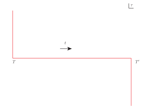
Figure 2.1: Son-Starinets prescription is equivalent to performing path integral on vacuum-to-vacuum contour in the complex time plane, as depicted above. The vacuum state is obtained by projection in the Euclidean path integral.

In Chapter 7, using gauge/gravity duality, we calculate the symmetric two-point function of the strongly coupled ${\cal N}=4$ Super Yang-Mills as a function of the geodesic distance. Here, we will focus only on the ${\mathbb{Z}}_{N}$-invariant phase, which corresponds to the topological black hole geometry. We find that there is an ambiguity in the two-point function that arises from the vacuum ambiguity of the boundary field theory. From the bulk point of view, this ambiguity comes from the fact that there are an infinite family of bulk radial wave functions that are normalizable deep into the bulk, at the horizon of the topological AdS black hole Balasubramanian:1998de .

Thus, the strongly coupled ${\cal N}=4$ Super Yang-Mills on $dS_{3}$ has an infinite class of symmetric two-point functions, parametrized by a set of complex parameters $\{\alpha_{\nu}\}$. This is different from the case of the weakly coupled theory, where the infinite family of symmetric two-point functions is parametrized by a single complex parameter $\alpha$. One possible explanation is that as one increases the coupling constant of the theory, going from the free theory toward the strongly coupled one, the $\alpha$-vacua mix with one another.

In order to be self-contained, before going to the detailed calculations on the asymptotically locally anti de Sitter spacetimes with de Sitter boundary, we will start this part of the thesis by reviewing some aspects of gauge/gravity duality that will be important in our calculation. We will then end this part of the thesis with some discussions and open questions in Chapter 8.

[15pc] Just as we have two eyes and two feet, duality is part of life. Carlos Santana (b. 1947)

3 Aspects of Gauge/gravity Duality

3.1 The Correspondence

The gauge/gravity duality is defined by the relation

$$\int_{\Phi\rightarrow\Phi_{0}}\,{\cal D}\Phi\,e^{i\,S_{\rm grav}[\Phi]}=Z_{\rm gauge}[\partial M,\Phi_{0}],$$ (3.1)

where the right hand side is the generating functional of the gauge theory. The boundary values $\Phi_{0}$ of the fields $\Phi$ of the gravity theory are kept fixed and they become the source for their dual operators ${\cal O}$ in the gauge theory side. In particular, the boundary value of the expectation value of the metric becomes the spacetime $\partial M$ the gauge theory lives in.

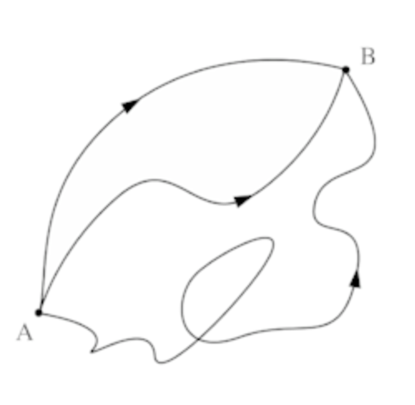
Figure 3.1: Path integral of a point particle moving in space starting at point A and ending at point B.

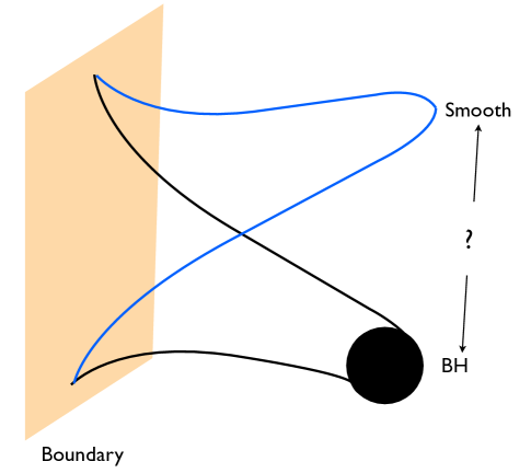
Figure 3.2: Path integral of spacetimes with boundary. Topology changing processes are included and such processes might go through a regime where the notion of spacetime itself is not valid.

The path integral on the left hand side of Eq. 3.1 is the full non-perturbative description of a quantum theory of gravity. In order to appreciate this more fully, let us recall the definition of path integral for a point particle moving in space. The boundary values for the position field at initial and final time are given (i.e., kept fixed) while in between (i.e., deep in the “bulk”), the position field is allowed to fluctuate and to take any possible values. This is depicted in Fig. 3.1. Similarly, in gauge/gravity duality, the boundary spacetime and boundary values of other fields are kept fixed, but they are allowed to fluctuate in the bulk (see Fig. 3.2). In particular, the bulk spacetime can be smooth or it can have a horizon. The process in which the bulk spacetime changes its topology from one to another is encoded in the path integral. It is also possible that this transition will go through a regime in which the notion of spacetime itself is no longer valid.

Remarkably, the complicated gravity path integral can be expressed as something that is rather simpler and somewhat more familiar: a generating functional of a gauge theory. The latter is a quantum field theory on a fixed classical spacetime, i.e., it is a theory without gravity. Therefore, it can be said that gravity is emergent and that parts of the bulk geometry are emergent too. For example, let us consider the gauge/gravity duality that involves Type IIB superstring theory on $AdS_{5}\times S^{5}$. The gravity theory is dual to ${\cal N}=4$ Super Yang-Mills living on a four-dimensional Minkowski space. The radial direction of the $AdS_{5}$ emerges from the renormalization group flow of the boundary theory, while the five-dimensional sphere emerges from the R-symmetry of the ${\cal N}=4$ Super Yang-Mills. For further study on how spatial dimensions and gravity might emerge from gauge theories, see for example Berenstein:2005aa ; Gursoy:2007np ; Berenstein:2007wi ; Berenstein:2007kq . On the issue of how the locality of the bulk physics might emerge, see for example Gary:2009ae ; Heemskerk:2009pn .

Gauge/gravity duality has also been used to understand the quantum gravity of black holes, in particular the issue of information paradox. In this approach, it has been realized that the black hole horizon geometry itself arises as an effective description. This is the key to solving the information paradox. For reviews, see for example Mathur:2008nj ; Balasubramanian:2008da .

In the semi-classical regime, we can evaluate the gravity path integral using saddle point approximation

$$\int_{\Phi\rightarrow\Phi_{0}}\,{\cal D}\Phi\,e^{i\,S_{\rm grav}[\Phi]}\approx\sum_{i}\int_{\Phi[\partial M]=\Phi_{0}}\,{\cal D}\Phi\,\,\exp\left(i\,\int_{M_{i}}{\cal L}[\Phi]\right),$$ (3.2)

where the sum in the right hand side is over bulk classical geometries $M_{i}$, whose boundary is $\partial M$. In other words, in this regime, the full non-perturbative gravity path integral has been reduced to the sum of perturbative gravity path integrals around fixed spacetimes. These spacetimes corresponds to different phases of the boundary field theory.

This regime corresponds to the gauge theory having a large rank gauge group and strong coupling constant. In particular, using this correspondence, we are able to obtain the leading order results of the boundary gauge theory, by merely perform classical gravitational calculations. Here, leading order means leading order in the $1/N$ expansion, where $N$ is the rank of the gauge group. Therefore, in this regime, gauge/gravity duality has become a powerful tool to study strongly coupled gauge theories. Its application encompasses the study of quark gluon plasma and strongly correlated condensed matter systems. Later in Chapter 7, we will see how to use gauge/gravity duality to try to address an issue in understanding inflationary cosmology, namely the issue of vacuum ambiguity in de Sitter space.

3.2 Building Dualities

In the previous section, we have given a general definition of gauge/gravity duality. However, in order to be able to perform calculations, we need a specific example of a specific gravity theory that is dual to a specific gauge theory. One way to build such a duality is by brane construction. We can construct a given gauge theory from the open string sector of a brane configuration by stacking and/or intersecting branes on a certain spacetime. If we increase the number of branes, the branes will backreact and the near horizon geometry of the backreacted spacetime will be the geometry that the (strongly coupled) field theory is dual to. If the field theory has more than one phase, the other phases will correspond to other geometries that have the same boundary as the near horizon geometry we just found.

3.2.1 Type IIB Superstring in $AdS_{5}\times S^{5}$ and ${\cal N}=4$ Super Yang-Mills

A canonical example involves Type IIB superstring theory. This theory has ${\cal N}=2$ supersymmetry and lives in 10 dimension. The low energy spectrum consists of:

• metric/graviton $g_{\mu\nu}$,

• dilaton $\phi$, which is a scalar field,

• axion $C_{0}$, which is a pseudo-scalar field,

• 2-form field $B_{\mu\nu}+iA_{2\mu\nu}$,

• 4-form field $A_{4\mu\nu\rho\sigma}$,

• gravitino $\psi_{\mu}$, which is a Majorana-Weyl fermion,

• dilatino $\lambda$, which is also a Majorana-Weyl fermion.

For more details, see for example Polchinski:1998rr .

It is natural to couple a $(p+1)$-form to an object $\Sigma_{p+1}$ of spacetime dimension $p+1$. The action can be constructed as follows

$$S_{p+1}=T_{p+1}\int_{\Sigma_{p+1}}A_{p+1},$$ (3.3)

where $T_{p+1}$ is the charge of this object under the $U(1)$ gauge group of the $(p+1)$-form. When this $(p+1)$-form is the Ramond-Ramond form field, the object $\Sigma_{p+1}$ is the D$p$-brane, a solitonic object at which open string can end (for more details, see for example Johnson:2003gi ). Related to the rank of the Ramond-Ramond form fields, D-branes in Type IIA superstring theory have even number of spatial dimensions, while those in Type IIB superstring theory have odd number of spatial dimensions.

Let us now consider a stack of $N$ D3-branes on a ten dimensional Minkowski space. Analyzing the open strings that end on this stack of D3-branes, we can see that the physics of these D3-branes is described by an ${\cal N}=4$ Super Yang-Mills living in a four-dimensional Minkowski space. The gauge group is $U(N)$, with the $U(1)$ factor corresponds to the overall position of the stack of the D3-branes. The gauge coupling constant is related to the string coupling constant by

$$g_{YM}^{2}=g_{s}.$$ (3.4)

For large $N$, the ten dimensional spacetime is no longer flat and the backreacted geometry is given by

$$ds^{2}=\left(1+\frac{L^{4}}{y^{4}}\right)^{-1/2}\eta_{\mu\nu}\,dx^{\mu}dx^{\nu}+\left(1+\frac{L^{4}}{y^{4}}\right)^{1/2}\left(dy^{2}+y^{2}d\Omega_{5}^{2}\right),$$ (3.5)

where

$$L^{4}=4\pi\,g_{s}\,N\,(\alpha^{\prime})^{2}.$$ (3.6)

Here, $1/2\pi\alpha^{\prime}$ is the string tension.

The near horizon geometry is obtained by taking a large $u$ limit, where

$$z\equiv\frac{L^{2}}{y},$$ (3.7)

and it is given by

$$ds^{2}=L^{2}\left[\frac{dz^{2}+\eta_{\mu\nu}\,dx^{\mu}dx^{\nu}}{z^{2}}+d\Omega^{2}_{5}\right].$$ (3.8)

This is a product geometry with one component is given by the hyperbolic space $AdS_{5}$, while the other component is a five dimensional sphere $S^{5}$, with L becoming the radius for both the AdS space and the sphere. Therefore, the physics close to the surface of the stack of D3-branes is given by Type IIB superstring theory living in $AdS_{5}\times S^{5}$. This should be equivalent to the physics described by the open string, modulo the spatial translation perpendicular to the D3-branes. Therefore, Type IIB superstring theory living in $AdS_{5}\times S^{5}$ is dual to ${\cal N}=4$ Super Yang-Mills living in a four-dimensional Minkowski space with $U(N)/U(1)\sim SU(N)$ gauge group.

The ${\cal N}=4$ Super Yang-Mills is a conformal theory. Combining the conformal symmetry and supersymmetry, it can be shown that the continuous global symmetry of this theory is the so-called superconformal group $SU(2,2|4)$. The maximal bosonic subgroup of the superconformal group is $SU(2,2)\times SU(4)_{R}\sim SO(2,4)\times SO(6)_{R}$. The conformal symmetry $SO(2,4)$ matches to the isometry of $AdS_{5}$, while the R-symmetry $SO(6)_{R}$ matches to the isometry of $S^{5}$. Combining this with the supersymmetry of the bulk theory, it can be shown that the gravity side also enjoys the full $SU(2,2|4)$ symmetry. Since the symmetry matches on both sides of the correspondence, it is then straightforward to establish a dictionary by matching a representation of the symmetry group $SU(2,2|4)$ of one side of the correspondence to the representation of the other side.

We note that when

$$\frac{L^{4}}{(\alpha^{\prime})^{2}}=4\pi\,g^{2}_{YM}\,N\,\gg 1$$ (3.9)

the gravity theory is well described by the Type IIB supergravity, which is the low energy description of the perturbative string theory. Therefore, at large $N$ and large t’Hooft coupling $\lambda=g^{2}_{YM}\,N$, the boundary field theory is dual to the Type IIB supergravity living in $AdS_{5}\times S^{5}$. In general, when the scale of the bulk geometry is larger than the string scale, or correspondingly at large $N$ and large t’Hooft coupling $\lambda$, we do not need the full non-perturbative string theory description and the gravity path integral is reduced to the sum of perturbative string theory/supergravity on fixed backgrounds.

3.2.2 AdS Black Hole, Thermal AdS Space and Thermal ${\cal N}=4$ Super Yang-Mills

A more complicated example can be obtained by putting the ${\cal N}=4$ Super Yang-Mills on a three-dimensional sphere and by switching on the temperature. The boundary geometry now becomes $S^{3}\times S^{1}$ with antiperiodic boundary conditions along the $S^{1}$ for the fermions.

There are two known geometries that have an $S^{3}\times S^{1}$ boundary, identified by Hawking and Page Hawking:1982dh . They are the so-called thermal AdS space and the Euclidean AdS Schwarzschild black hole. The thermal AdS space is a quotient of the Euclidean AdS space and the metric is given by

$$ds^{2}=f(r)\,dt^{2}+f(r)^{-1}\,dr^{2}+r^{2}d\Omega_{3}^{2},$$ (3.10)

where

$$f(r)=1+\frac{r^{2}}{R^{2}_{\rm AdS}},$$ (3.11)

and $t$ is a periodic coordinate with an arbitrary period $\beta$. As $\beta$ is the period of the circle at the boundary, it is identified as the inverse temperature of the boundary field theory.

The metric of the Euclidean AdS Schwarzschild black hole has the same form as the metric of thermal AdS 3.10, but with

$$f(r)=1+\frac{r^{2}}{R^{2}_{\rm AdS}}-\frac{M}{r^{2}}.$$ (3.12)

$M$ is related to the mass of the black hole $m_{\rm BH}$ as

$$M=\frac{8\,G_{N}}{3\pi}\,m_{\rm BH}.$$ (3.13)

There are two solutions to the equation $f(r)=0$: the larger solution $r_{+}$ is the radial position of the horizon of the so-called large AdS black hole and the smaller solution $r_{-}$ becomes the radial coordinate of the horizon of the small AdS black hole. It turns out that the small AdS black hole is unstable to perturbations. Furthermore, when viewed as a ten dimensional, asymptotically $AdS_{5}\times S^{5}$ solution smeared on the $S^{5}$, Ref. Hollowood:2006xb shows that the small AdS black hole is also unstable to localization on $S^{5}$, i.e., it suffers the Gregory-Laflamme instability.

The metric of the large AdS black hole is smooth and complete if and only if the period of $t$ is given by

$$\beta_{0}=\frac{2\pi R^{2}_{\rm AdS}r_{+}}{2r_{+}^{2}+R^{2}_{\rm AdS}}.$$ (3.14)

This is the inverse Hawking temperature of the black hole and is also identified with the temperature of the boundary field theory.

It turns out that the large AdS black hole corresponds to the plasma or deconfined phase of the thermal ${\cal N}=4$ Super Yang-Mills, while the thermal AdS space corresponds to the confined phase. Furthermore, the confinement-deconfinement phase transition of the boundary field theory corresponds to the Hawking-Page transition of the gravity theory. For more details, see for example Witten:1998zw ; Brandhuber:1998er ; Aharony:1999ti ; Aharony:2003sx .

3.3 Examples of Holographic Calculations

Above, we have given some examples of gauge/gravity duality. Now, let us consider some examples of holographic calculations in which we perform classical gravity calculations to obtain results for strongly coupled field theories.

3.3.1 Euclidean Calculation

Let us start with the simpler case of gauge/gravity duality with Euclidean signature. In Euclidean signature, the gauge/gravity correspondence defined in Eq. 3.1 becomes

$$Z_{\rm gauge}[\partial M,\Phi_{0}]=\int_{\Phi\rightarrow\Phi_{0}}\,{\cal D}\Phi\,e^{-\,S_{\rm grav}[\Phi]}\approx\sum_{i}Z_{\rm grav}[M_{i},\Phi],$$ (3.15)

where the left hand side is the partition function of the gauge field living on $\partial M$ with source $\Phi_{0}$, while the right hand side is the gravitational partition function summed over geometries $M_{i}$ whose boundary is $\partial M$ and the boundary values of the fields in the gravity theory are given by $\Phi(\partial M)=\Phi_{0}$.

Our goal is to study the strongly coupled field theory by calculating the correlation functions of its operators. The latter can be obtained by taking the appropriate derivatives of the gauge theory partition function with respect to the source $\Phi_{0}$ and then setting the source to zero. Even though it is very difficult to calculate the strongly coupled gauge theory partition function directly, the gauge/gravity correspondence tells us that this partition function is nothing but the gravity partition function with the fields in the gravitational theory having appropriate boundary conditions, namely $\Phi(\partial M)=\Phi_{0}$. We can obtain this gravity partition function by first solving the classical equations of motion of the fields with the boundary condition $\Phi(\partial M)=\Phi_{0}$.

To summarize, in order to study the strongly coupled field theory using holographic techniques, our strategy is as follows:

1. Solve the classical equations of motion of the bulk fields $\Phi$ subject to the boundary conditions $\Phi(\partial M)=\Phi_{0}$.

2. Substitute the solutions of step 1 into the Euclidean path integral.

3. The result of step 2 is the partition function for the gauge theory, where $\Phi_{0}$ being the source for the dual operator. By taking derivatives with respect to $\Phi_{0}$ and then setting $\Phi_{0}=0$, we obtain the correlation functions of the field theory operators ${\cal O}$.

Let us now consider a specific example of the duality between strongly coupled ${\cal N}=4$ Super Yang-Mills on a four-dimensional Euclidean flat space with classical Type IIB supergravity theory on a five-dimensional Euclidean AdS space (times the five-dimensional sphere).

For a reminder, the $AdS_{5}$ metric in is given by

$$ds^{2}={R_{\rm AdS}^{2}\over z^{2}}\left(dz^{2}+\delta_{\mu\nu}\,dx^{\mu}dx^{\nu}\right).$$ (3.16)

This metric does not describe the full $AdS_{5}$ geometry, but only the so-called Poincar$\acute{\rm e}$ patch. In this parametrization, the conformal boundary is at $z=0$, while the “origin” of the space is at $z\rightarrow\infty$.

Let us consider a scalar field $\phi$ with mass $m$ living in the bulk. The action is given by

$$S_{E}=\frac{N^{2}}{16\pi^{2}R_{\rm AdS}}\int d^{4}x\int dz\;\sqrt{g}\left(g^{MN}\,\partial_{M}\phi\,\partial_{N}\phi+m^{2}\phi^{2}\right).$$ (3.17)

Its equation of motion is given by

$$\left(\Box-m^{2}\right)\phi=0,$$ (3.18)

which translates to

$$z^{5}\,\partial_{z}\left({1\over z^{3}}\,\partial_{z}\phi\right)+z^{2}\,\partial_{\mu}\partial^{\mu}\phi-m^{2}R^{2}_{\rm AdS}\,\phi=0.$$ (3.19)

There are two independent solutions

$$\phi=z^{2}\;e^{-ik\cdot x}\;I_{\nu}(kz)\qquad{\rm and}\qquad\phi=z^{2}\;e^{-ik\cdot x}\;K_{\nu}(kz),$$ (3.20)

where the index of the modified Bessel functions $I_{\nu}$ and $K_{\nu}$ is given by

$$\nu=\sqrt{4+(m\,R_{\rm AdS})^{2}},$$ (3.21)

and $k$ in their argument is understood to be the magnitude $k=\sqrt{\delta_{\mu\nu}\,k^{\mu}k^{\nu}}$ of the boundary momentum.

Neither of the above solutions is square integrable, but only the second solution is smooth in the interior. Since there is no singularity in the interior, the physical solution will be

$$\phi=z^{2}\;\int{d^{4}k\over(2\pi)^{4}}\,C(k)\,e^{-ik\cdot x}\;K_{\nu}(kz),$$ (3.22)

where $C(k)$ is chosen such that the solution satisfies the boundary condition $\phi(z=0,x)=\phi_{0}(x)$. Substituting this solution into the Euclidean action, we get

$$S_{E}=\frac{N^{2}}{16\pi^{2}R_{\rm AdS}}\int d^{4}x\;g^{zz}\sqrt{g}\,\phi(x,z)\,\partial_{z}\phi(x,z)\big{|}_{z=0},$$ (3.23)

which diverges due to the divergent volume element at the boundary. We can regulate this by explicitly cutting off the AdS bulk geometry at $z=\epsilon$ and then taking $\epsilon\rightarrow 0$.

Denoting the boundary value of the field $\phi$ as

$$\phi_{0}(x)=\phi(\epsilon,x)=\int{d^{4}k\over(2\pi)^{4}}\,\bar{\phi}_{0}(k)\,e^{-ik\cdot x},$$ (3.24)

it is easy to see that the solution is now given by

$$\phi(z,x)=\int{d^{4}k\over(2\pi)^{4}}\,{z^{2}K_{\nu}(kz)\over\epsilon^{2}K_{\nu}(k\epsilon)}\,e^{-ik\cdot x}\,\bar{\phi}_{0}(k).$$ (3.25)

Substituting this solution into the Euclidean action, we get

$$S_{E} = \frac{N^{2}}{16\pi^{2}R_{\rm AdS}}\int d^{4}x\;g^{zz}\sqrt{g}\,\phi(x,z)\,\partial_{z}\phi(x,z)\big{|}_{z=\epsilon}$$

$$= \frac{N^{2}}{16\pi^{2}R_{\rm AdS}}\,{1\over\epsilon^{3}}\int{d^{4}p\over(2\pi)^{4}}\,{d^{4}q\over(2\pi)^{4}}\,\bar{\phi}_{0}(p)\Bigg{[}(2\pi)^{4}\,\delta^{(4)}(p+q)\,{d\over d\epsilon}\left(\ln\left[\epsilon^{2}K_{\nu}(p\epsilon)\right]\right)\Bigg{]}\bar{\phi}_{0}(q).$$

It is now straightforward to read off the Fourier transform of the regulated two-point function of the boundary field theory from this on-shell action and it is given by

$$\langle{\cal O}(p){\cal O}(q)\rangle = {\delta^{2}S_{E}\over\delta\bar{\phi}_{0}(p)\delta\bar{\phi}_{0}(q)}$$ (3.27)

$$= (2\pi)^{4}\,\delta^{(4)}(p+q)\,\frac{N^{2}}{8\pi^{2}R_{\rm AdS}}\,{1\over\epsilon^{3}}\,{d\over d\epsilon}\left(\ln\left[\epsilon^{2}K_{\nu}(p\epsilon)\right]\right).$$

For example, the lowest KK modes of the dilaton and axion of the Type IIB superstring theory, which are massless, minimally coupled scalar fields in $AdS_{5}$, lead to

$$\langle{\cal O}(p){\cal O}(-p)\rangle=\frac{N^{2}}{32\pi^{2}R_{\rm AdS}}\left(-{p^{2}\over\epsilon^{2}}-{p^{4}\over 2}\ln\left[p\epsilon\right]\right)+{\rm constants},$$ (3.28)

which is the two-point function the scalar glueball operators ${\rm Tr}\,F_{\mu\nu}F^{\mu\nu}$ and ${\rm Tr}\,F_{\mu\nu}\tilde{F}^{\mu\nu}$ of the ${\cal N}=4$ Super Yang-Mills theory. Fourier transforming back to position space, we get

$$\langle{\cal O}(x){\cal O}(x^{\prime})\rangle=\frac{N^{2}}{64\pi^{2}R_{\rm AdS}}\,\frac{1}{|x-x^{\prime}|^{8}},$$ (3.29)

which is a two-point function for dimension four operators in the conformal field theory. This confirms further that the dilaton and axion of the Type IIB superstring theory are dual to the scalar glueball operators of the ${\cal N}=4$ Super Yang-Mills theory ${\rm Tr}\,F_{\mu\nu}F^{\mu\nu}$ and ${\rm Tr}\,F_{\mu\nu}\tilde{F}^{\mu\nu}$, respectively.

In general, using the asymptotic behavior of the non-normalizable mode near the boundary, it can be shown that the relation between the mass $m$ of the bulk scalar field and the dimension $\Delta$ of the boundary field theory operator it is dual to is given by

$$m^{2}=\Delta(\Delta-4).$$ (3.30)

The divergent terms in Eq. 3.28, which depend on the UV cutoff of the boundary field theory, are the so-called contact terms. Contact terms are Fourier transforms of derivatives acting on Dirac delta function. For example, $p^{2}$ is the Fourier transform of $\Box\delta^{4}(x-x^{\prime})$. The divergences from these contact terms manifest themselves when the field theory operators we are considering lay on top of each other, i.e., when $x=x^{\prime}$.

3.3.2 Lorentzian Calculation

In the Euclidean case, with the help of the physical argument that the solution of the equation of motion should be smooth in the interior of the bulk, the solution to the equation of motion for the given boundary condition is unique. However, for the Lorentzian anti de Sitter spacetimes, fixing the boundary value of the field is not enough to warranty a unique solution. This is because there are two linearly independent solutions that are smooth in the interior Avis:1977yn . The variety of the radial parts of the solution to the equation of motion of the gravity theory is related to the variety of real time correlators of the boundary field theory. The latter is the result of two things:

• the multitude of real time Green’s functions, i.e., retarded, advanced, etc;

• the possibility of vacuum ambiguity, especially if the boundary manifold is time-dependent.

In this section, we will review Son and Starinets’ prescription on how to obtain the retarded correlators for the boundary field theory Son:2002sd . If the boundary field theory suffers from vacuum ambiguity, this prescription will also choose the vacuum obtained by Euclidean projection vanRees:2009rw , as depicted in Fig. 2.1. This prescription is especially suitable for calculations involving black holes. In order to obtain the retarded propagator, the prescription requires infalling boundary condition at the horizon, while the advanced propagator corresponds to the outgoing boundary condition at the horizon.

3.3.2.1 Retarded Correlators for the Scalar Glueball Operators

To study the Lorentzian AdS/CFT duality, let us consider the near-horizon geometry of a stack of three-dimensional near extremal branes. It is equivalent to the Lorentzian AdS Schwarzschild black hole in the large mass limit and the metric is given by

$$ds^{2}=\frac{R_{\rm AdS}^{2}}{z^{2}}\left(-f(z)dt^{2}+d\vec{x}^{2}+f(z)^{-1}dz^{2}\right),$$ (3.31)

where

$$f(z)=1-\frac{z^{4}}{z^{4}_{H}}.$$ (3.32)

The boundary is at $z=0$ and the horizon is at $z=z_{H}$, with $z_{H}=1/\pi T$, $T$ being the Hawking temperature.

The Lorentzian $AdS_{5}$ can then be considered as the $T\rightarrow 0$ limit of the geometry 3.31 and we can apply the Son-Starinets prescription to obtain the retarded propagator of the strongly coupled ${\cal N}=4$ Super Yang-Mills.

For spacelike boundary momenta $k^{2}>0$, the calculation is identical to the Euclidean case we considered before, but with an extra minus sign in front of the Lorentzian action. The answer is given by

$$G_{R}(k)=\frac{N^{2}\,k^{4}}{64\pi^{2}R_{\rm AdS}}\,\ln k^{2}.$$ (3.33)

For timelike boundary momenta $k^{2}<0$, we can obtain the retarded correlator by requiring the solution to take the incoming wave form at $z=0$, which can be viewed as the “point” or vanishing horizon. Introducing $q=\sqrt{-k^{2}}$, the solution for the equation of motion is

$$\phi(z,x)\;=\;\int{d^{4}k\over(2\pi)^{4}}\,e^{-ik\cdot x}\,\bar{\phi}_{0}(k)\,\begin{cases}\displaystyle{{z^{2}H_{\nu}^{(1)}(qz)\over\epsilon^{2}H_{\nu}^{(1)}(q\epsilon)}\,,}&\omega>0,\cr\vskip 4.0pt\cr\displaystyle{{z^{2}H_{\nu}^{(2)}(qz)\over\epsilon^{2}H_{\nu}^{(2)}(q\epsilon)}\,,}&\omega<0.\cr\end{cases}$$ (3.34)

As before,

$$\nu=\sqrt{4+(m\,R_{\rm AdS})^{2}},$$ (3.35)

and $\omega$ is the time component of $k$.

Substituting the solution into the action, we can read the retarded propagator

$$G_{R}(k)={N^{2}k^{4}\over 64\pi^{2}}(\ln{k^{2}}-i\pi\,\mbox{sgn}\,\omega)\,.$$ (3.36)

From this result, we can then obtain the Feynman propagator

$$G_{F}(k)={N^{2}k^{4}\over 64\pi^{2}}(\ln{|k^{2}|}-i\pi\,\theta(-k^{2}))\,,$$ (3.37)

which can be obtained from the Euclidean correlator

$$G_{E}(k_{E})=-{N^{2}k_{E}^{4}\over 64\pi^{2}}\ln{k_{E}^{2}}$$ (3.38)

by analytical continuation.

3.3.2.2 Retarded R-charge Current Correlators

The massive AdS Schwarzschild black hole geometry 3.31 is interesting in its own right as it can be used to learn the transport property of the strongly coupled plasma of the ${\cal N}=4$ Super Yang-Mills. To do so, let us consider a $U(1)$ gauge field living in the bulk whose action is given by

$$S=-\frac{N^{2}}{64\pi^{2}R_{\rm AdS}}\int d^{5}x\sqrt{-g}g^{\mu\alpha}g^{\nu\beta}F_{\mu\nu}F_{\alpha\beta}\,.$$ (3.39)

This field is obtained by compactifying around the $S^{5}$ the gauge field whose gauge field strength is the Hodge dual of the field strength of the 2-form field. This $U(1)$ gauge field $A^{\mu}$ corresponds to the R-current $j^{\mu}$ of the boundary field theory, which is a conserved current. From the R-charge correlator, we can then read the diffusion constant of the strongly coupled plasma.

Without losing any generality, we can align the R-charge perturbation to carry the spatial momentum along the $x^{3}$-axis, i.e., $p=(\omega,0,0,k)$. Furthermore, we can use gauge freedom to set the radial component of the gauge potential $A_{z}=0$. Hence, from the symmetries of the configuration, there are two remaining bulk gauge fields that are non zero and they can be written as

$$A_{0}=e^{-ip\cdot x}\,\tilde{A}_{0}(z,p)\qquad{\rm and}\qquad A_{3}=e^{-ip\cdot x}\,\tilde{A}_{3}(z,p).$$ (3.40)

It is convenient to introduce an alternative radial coordinate $u=z_{H}^{2}/z^{2}$. In this parametrization, the Maxwell equations can be written as

$$w\tilde{A}_{0}^{\prime}+qf\tilde{A}_{3}^{\prime} = 0\,,$$ (3.41)

$$\tilde{A}_{0}^{\prime\prime}-\frac{1}{uf}(q^{2}\tilde{A}_{0}+wq\tilde{A}_{3}) = 0\,,$$ (3.42)

$$\tilde{A}_{3}^{\prime\prime}+\frac{f^{\prime}}{f}\tilde{A}_{3}^{\prime}+\frac{1}{uf^{2}}(w^{2}\tilde{A}_{3}+wq\tilde{A}_{0}) = 0\,,$$ (3.43)

where ^′ denotes a derivative with respect to $u$ and we have introduced dimensionless quantities

$$w=\frac{\omega}{2\pi T}\qquad{\rm and}\qquad q=\frac{k}{2\pi T}.$$ (3.44)

We can eliminate $\tilde{A}_{3}$ and obtain a third-order differential equation for $\tilde{A}_{0}$,

$$\tilde{A}_{0}^{\prime\prime\prime}+\frac{(uf)^{\prime}}{uf}\tilde{A}_{0}^{\prime\prime}+\frac{w^{2}-q^{2}f}{uf^{2}}\tilde{A}_{0}^{\prime}=0\,,$$ (3.45)

which we only need to solve for $\tilde{A}_{0}^{\prime}$ due to the fact that the action only depends on $\tilde{A}_{0}^{\prime}$ and not $\tilde{A}_{0}$. The full solution is not known, but fortunately, we do not need to know the full solution to learn about the transport property of the strongly coupled plasma. To do so, we only need to know the solution for small energy and momentum, which we can obtain perturbatively in $w$ and $q^{2}$.

Near the horizon $u=1$, there are two independent solutions, $\tilde{A}_{0}^{\prime}\propto(1-u)^{\pm iw/2}$, but the incoming wave boundary condition singles out the solution that behaves like $(1-u)^{-iw/2}$ near the horizon. Our ansatz is then

$$\tilde{A}_{0}^{\prime}=(1-u)^{-iw/2}\left(g_{0,0}+g_{1,0}\,\frac{iw}{2}+g_{0,1}\,q^{2}+\cdots\right),$$ (3.46)

whose coefficients can be obtained by requiring that the solution has no extra singularities at the horizon.

At leading order, we have

$$\frac{1-3u^{2}}{u-u^{3}}\,g_{0,0}^{\prime}+g_{0,0}^{\prime\prime}=0,$$ (3.47)

whose solution is

$$g_{0,0}=C_{1}+\frac{C_{2}}{2}\ln\frac{u^{2}-1}{u^{2}}.$$ (3.48)

The regularity condition at the horizon enforces $C_{2}=0$.

At ${\cal O}(w)$, we have

$$-(1+2u)C_{1}+(3u^{2}-1)\,g^{\prime}_{1,0}+u(u^{2}-1)\,g_{1,0}^{\prime\prime}=0,$$ (3.49)

whose solution is

$$g_{1,0}=C_{1}\ln(u-1)+C_{3}+\frac{C_{4}}{2}\ln\frac{u^{2}-1}{u^{2}}.$$ (3.50)

In order for the solution not to have extra singularities, we must have

$$C_{3}=C_{1}\ln 2\qquad{\rm and}\qquad C_{4}=-2C_{1}.$$ (3.51)

Finally, at ${\cal O}(q^{2})$, we have

$$C_{1}+(3u^{2}-1)\,g_{0,1}^{\prime}+u(u^{2}-1)\,g_{0,1}^{\prime\prime}=0,$$ (3.52)

whose solution is

$$g_{0,1}=C_{5}-\frac{C_{1}-C_{6}}{2}\ln(u-1)+\frac{C_{1}+C_{6}}{2}\ln(u+1)-C_{6}\ln u.$$ (3.53)

Again, requiring the same condition as above, we get

$$C_{5}=-C_{1}\ln 2\qquad{\rm and}\qquad C_{6}=C_{1}.$$ (3.54)

Using Eq. (3.42), we can express $C_{1}$ in terms of the boundary values of $\tilde{A}_{0}$ and $\tilde{A}_{3}$ at $u=0$, namely

$$C_{1}=\left.\frac{q^{2}\tilde{A}_{0}+wq\tilde{A}_{3}}{iw-q^{2}}\right|_{u=0}\,.$$ (3.55)

Differentiating the on-shell Maxwell action with respect to the boundary values, we can find the R-current correlators. In particular,

$$\langle j_{0}(p)\,j_{0}(-p)\rangle=\frac{N^{2}T}{16\pi}\frac{k^{2}}{i\omega-Dk^{2}}\,,$$ (3.56)

where

$$D=\frac{1}{2\pi T}\,.$$ (3.57)

The correlator given by Eq. (3.56) has a hydrodynamic diffusive pole and $D$ is the R-charge diffusion constant (for a treatment of relativistic fluid dynamics, see for example LL6 ).

[15pc] Boundaries are actually the main factor in space, just as the present, another boundary, is the main factor in time. Eduardo Chillida (1924 - 2002)

4 Anti de Sitter Spacetimes with de Sitter Boundary

In this chapter, we review the geometries involved in the holographic calculation. Before reviewing the anti de Sitter spacetimes with de Sitter boundary, let us start by reviewing some properties of de Sitter space.

4.1 The de Sitter Space

The de Sitter space is the maximally symmetric solution to Einstein equation with positive cosmological constant. It can be viewed as a “sphere” described by

$$-x_{0}^{2}+x_{1}^{2}+\cdots+x_{d}^{2}=R_{\rm dS}^{2}$$ (4.1)

in a flat $d{+}1$-dimensional Minkowski space, where $R_{\rm dS}$ is a parameter with unit of length, which we will call the de Sitter radius. The relation between the de Sitter radius and the cosmological constant $\Lambda$ is given by

$$\Lambda={(d-2)(d-1)\over 2\,R_{\rm dS}^{2}}.$$ (4.2)

We note that in the embedding 4.1 the O$(d,1)$ symmetry, which is the isometry group of $dS_{d}$, is manifest. We will sometime refer to this symmetry as the de Sitter symmetry.

The metric for the global patch can be obtained by setting

$$x^{0} = R_{\rm dS}\,\sinh\frac{t}{R_{\rm dS}},$$ (4.3)

$$x^{i} = R_{\rm dS}\,\omega^{i}\,\cosh\frac{t}{R_{\rm dS}},\leavevmode\nobreak\ \leavevmode\nobreak\ \leavevmode\nobreak\ \leavevmode\nobreak\ \leavevmode\nobreak\ i=1,\ldots,d,$$ (4.4)

where $\omega_{i}$’s form a coordinate for a $d-1$-dimensional sphere $S^{d-1}$

$$\omega^{1} = \cos\theta_{1},$$ (4.5)

$$\omega^{2} = \sin\theta_{1}\cos\theta_{2},$$ (4.6)

$$\vdots$$ (4.7)

$$\omega^{d-1} = \sin\theta_{1}\cdots\sin\theta_{d-2}\cos\theta_{d-1},$$ (4.8)

$$\omega^{d} = \sin\theta_{1}\cdots\sin\theta_{d-2}\sin\theta_{d-1},$$ (4.9)

where $0\leq\theta_{i}<\pi$ for $1\leq i<d-1$, but $0\leq\theta_{d-1}<2\pi$. The metric is given by

$$ds^{2}=-dt^{2}+R_{\rm dS}^{2}\cosh^{2}\left({t\over R_{\rm dS}}\right)\;d\Omega_{d-1}^{2}.$$ (4.10)

In these coordinates, the $d$-dimensional de Sitter space looks like a $d{-}1$-dimensional sphere which starts out infinitely large at $t=-\infty$, then shrinks to a minimal finite size at $\tau=0$, then grows again to infinite size as $t\to+\infty$.

We note that $\partial_{t}$ is not a Killing vector and there is no globally time-like Killing vector in de Sitter space. This absence of a globally time-like Killing vector in de Sitter space is tightly related to the issue of vacuum ambiguity of field theories on de Sitter space. We will discuss this issue of vacuum ambiguity in Chapter 7.

4.2 The Topological AdS Black Hole

The so-called topological black hole in $AdS_{5}$ (times a five-dimensional sphere) can be obtained as a near horizon limit of $N$ D3-branes filling a boost orbifold ${\mathbb{R}}^{1,1}/{\mathbb{Z}}$ Balasubramanian:2005bg . It is an orbifold of the $AdS_{5}$ space, obtained by an identification of points along the orbit of a Killing vector

$$\xi=\frac{r_{\chi}}{R_{\rm AdS}}\left(x_{4}\partial_{5}+x_{5}\partial_{4}\right),$$ (4.11)

where $r_{\chi}$ is an arbitrary real number and the $AdS_{5}$ is described as the universal covering of the hypersurface

$$-x_{0}^{2}+x_{1}^{2}+x_{2}^{2}+x_{3}^{2}+x_{4}^{2}-x_{5}^{2}=-R^{2}_{\rm AdS},$$ (4.12)

$R_{\rm AdS}$ being the $AdS_{5}$ radius. In Kruskal-like coordinates, which cover the whole spacetime, the metric has the form

$$ds^{2}={4R^{2}_{\rm AdS}\over(1-y^{2})^{2}}\;dy^{\mu}dy^{\nu}\eta_{\mu\nu}+{(1+y^{2})^{2}\over(1-y^{2})^{2}}\;r_{\chi}^{2}d\chi^{2},$$ (4.13)

where $\chi$ is a periodic coordinate with period $2\pi$. The four coordinates $y^{\mu}$, with $\mu=0,\ldots 3$, are non-compact, with the Lorentzian norm $y^{2}=y^{\mu}y^{\nu}\eta_{\mu\nu}$ is between -1 and 1. Locally, the spacetime is anti de Sitter with a periodic identification of the $\chi$ coordinate,

$$\chi\sim\chi+2\pi.$$ (4.14)

The conformal boundary of the spacetime is approached as $y^{2}\rightarrow 1$, and it is $dS_{3}\times S^{1}$. The boundary conformal field theory is therefore formulated on a three dimensional de Sitter space with radius of curvature $R_{\rm AdS}$ times a spatial circle of radius $r_{\chi}$.

The geometry has a horizon at $y^{2}=0$, which is the three dimensional hypercone,

$$y_{0}^{2}=y_{1}^{2}+y_{2}^{2}+y_{3}^{2},$$ (4.15)

and a singularity at $y^{2}=-1$. The hyperboloid $y^{2}=-1$ is a singularity since timelike geodesics end there and the Killing vector $\partial_{\chi}$ generating the orbifold identification has vanishing norm at $y^{2}=-1$. This singularity appears because the region where the Killing vector has negative norm needs to be excised from the physical spacetime to eliminate closed timelike curves.

It is interesting to see that we can get a better understanding of the geometry in the vicinity of the singularity at $y^{2}=-1$ by zooming in on the the metric (4.13) in this region. Introducing the coordinates

$$y_{0}=(1-\delta)\,\cosh\varepsilon\,,\qquad Y=(1-\delta)\,\sinh\varepsilon\qquad 0<\delta\ll 1,$$ (4.16)

we find

$$ds^{2}\approx R^{2}_{\rm AdS}(-d\delta^{2}+d\varepsilon^{2}+\sinh^{2}\varepsilon\,d\Omega_{2}^{2})+r_{\chi}^{2}\delta^{2}\,d\chi^{2},$$ (4.17)

which is a product of geometries, with the factor in the $\delta,\chi$ directions is describing the Milne spacetime.

The topology of the spacetime is ${\mathbb{R}}^{3,1}\times S^{1}$, in contrast to that of the AdS-Schwarzschild black hole, which has the topology ${\mathbb{R}}^{1,1}\times S^{3}$. For this reason, in this geometry, infinity is connected, unlike in the usual Schwarzschild black hole which has two disconnected asymptotic regions.

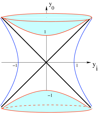
Figure 4.1: The global structure of the topological AdS black hole spacetime. The singularity is the hyperboloid $-y_{0}^{2}+y_{i}y_{i}=-1$ and the horizon is at the cone $y_{0}^{2}=y_{i}y_{i}$.

It is possible to rewrite the metric in Schwarzschild-like coordinates by introducing the following coordinate transformations

$$Y^{2}=\sum_{i=1}^{3}y_{i}y_{i}\,;\qquad{Y\over y_{0}}=\coth\left({t\over R_{\rm AdS}}\right)\,;\qquad{r^{2}\over R^{2}_{\rm AdS}}=4{(Y^{2}-y_{0}^{2})\over(1+y_{0}^{2}-Y^{2})^{2}}.$$ (4.18)

These coordinates only cover the exterior of the topological black hole $y^{2}\geq 0$. Locally, the metric takes the form

$$\begin{split}ds^{2}={R^{2}_{\rm AdS}\,dr^{2}\over(r^{2}+R^{2}_{\rm AdS})}+\left({r_{\chi}\over R_{\rm AdS}}\right)^{2}(r^{2}+R^{2}_{\rm AdS})d\chi^{2}+\frac{r^{2}}{R_{\rm AdS}^{2}}\left(-dt^{2}+R_{\rm AdS}^{2}\,\cosh^{2}\left({t\over R_{\rm AdS}}\right)\;d\Omega_{2}^{2}\right).\end{split}$$ (4.19)

The Euclidean continuation of this metric yields the thermal AdS space. Hence, the metric of the exterior region of the topological black hole can also be obtained following a double Wick rotation of global AdS spacetime and a periodic identification of the $\chi$ coordinate.

In the Schwarzschild-like coordinates, the horizon of the topological black hole is at $r=0$, while the boundary is at $r\rightarrow\infty$. It is clear that each slice of constant $r$ is a $dS_{3}\times S^{1}$ geometry, where the three-dimensional de Sitter space is in the global patch. The metric (4.19), while locally describing AdS space, differs from it globally due to the identification ${\chi\sim\chi+2\pi}$. We note also that the spatial $S^{1}$ remains finite sized at the horizon, with radius $R_{S^{1}}=r_{\chi}$.

It will also be convenient to introduce a dimensionless radial coordinate $z=R_{\rm AdS}/r$, in which the metric for the exterior region is now given by

$$ds^{2}=R^{2}_{\rm AdS}\left[{dz^{2}\over z^{2}(z^{2}+1)}+{1\over z^{2}}\left(-{dt^{2}\over R_{\rm AdS}^{2}}+\cosh^{2}\left({t\over R_{\rm AdS}}\right)\;d\Omega_{2}^{2}\right)+\frac{1+z^{2}}{z^{2}}\left({r_{\chi}\over R_{\rm AdS}}\right)^{2}d\chi^{2}\right].$$ (4.20)

Here, the boundary is at $z=0$, while the horizon is at $z\rightarrow\infty$.

If the bulk fermions have anti-periodic boundary conditions in the $\chi$-direction, then the topological black hole has a semiclassical instability when

$$r_{\chi}<{R_{\rm AdS}\over 2\sqrt{2}}\,,$$ (4.21)

which causes it to decay into the AdS bubble of nothing Balasubramanian:2005bg . The instability only occurs if fermions have antiperiodic boundary conditions in the $\chi$-direction. With periodic boundary conditions for both bosons and fermions, the topological AdS black hole is absolutely stable. This instability can also be seen in the boundary field theory by considering the effective potential of the Polyakov loop of the Euclidean field theory Hollowood:2006xb .

4.3 The AdS Bubble of Nothing

As originally pointed out in Witten:1981gj (and Balasubramanian:2005bg , in the present context), the decay of a false vacuum in semiclassical gravity is computed by the Euclidean bounce which has the same asymptotics as the false vacuum in Euclidean signature. The bounce is a solution to the Euclidean equations of motion with a non-conformal negative mode. In the context of the asymptotically locally AdS spaces in question, the small Euclidean Schwarzschild solution represents such a bounce solution. In Lorentzian signature, the semiclassical picture of the decay process at say, time $t=0$ involves replacing the $t>0$ part of the false vacuum solution, i.e., the topological black hole solution, with the appropriate analytic continuation of the Euclidean bounce to Lorentzian signature. The analytic continuation of the small Euclidean AdS black hole bounce which leads to $dS_{3}\times S^{1}$ boundary asymptotics is the (small) AdS bubble of nothing.

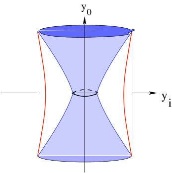
Fig. 4.2: The global structure of the bubble geometry. The region inside the shaded region is empty, and its surface represents the de Sitter expansion of the bubble at $r=r_{h}$.

The metric for the AdS bubble of nothing solution is

$$ds^{2}=f(r)\;r_{\chi}^{2}\;d\chi^{2}+f(r)^{-1}\;dr^{2}+{r^{2}\over R_{\rm AdS^{2}}}\left(-dt^{2}+\cosh^{2}\left({t\over R_{\rm AdS}}\right)d\Omega_{2}^{2}\right),$$ (4.22)

where

$$f(r)=1+{r^{2}\over R_{\rm AdS}^{2}}-{r_{h}^{2}(R_{\rm AdS}^{2}+r_{h}^{2})\over r^{2}}.$$ (4.23)

In order to avoid a conical singularity in the interior, the periodicity of the compact $\chi$ coordinate is related to $r_{h}$ as

$$2\pi r_{\chi}=2\pi R^{2}_{\rm AdS}\;{r_{h}\over r_{h}^{2}+R_{\rm AdS}^{2}}.$$ (4.24)

Passing to the dimensionless coordinates

$$\rho=\sqrt{(r/R_{\rm AdS})^{2}+1},\qquad\tau={t\over R_{\rm AdS}},\qquad\tilde{r}_{h}={r_{h}\over R_{\rm AdS}},$$ (4.25)

the metric becomes

$$ds^{2}=R^{2}_{\rm AdS}\left[\tilde{f}(\rho)\;{r_{\chi}^{2}\over R^{2}_{\rm AdS}}\;d\chi^{2}+\tilde{f}(\rho)^{-1}\;{\rho^{2}\over\rho^{2}-1}\;d\rho^{2}+(\rho^{2}-1)(-d\tau^{2}+\cosh^{2}\tau d\Omega_{2}^{2})\right],$$ (4.26)

where

$$\tilde{f}(\rho)=\rho^{2}-{1\over\rho^{2}-1}\;{\tilde{r}_{h}^{2}}\;\left(\tilde{r}_{h}^{2}+1\right).$$ (4.27)

In the AdS bubble of nothing spacetime, a slice of constant $\rho$ is $dS_{3}\times S^{1}$. The $S^{1}$, however, shrinks to zero size smoothly at $\rho=\sqrt{\tilde{r}_{h}^{2}+1}$. The shrinking circle is the cigar of the Euclidean Schwarzschild solution. The boundary of the spacetime is approached as $\rho\rightarrow\infty$. The semiclassical decay of the topological black hole at $\tau=0$, results in the sudden appearance of a bubble of nothing in the region of spacetime, $\rho^{2}\leq 1+\tilde{r}_{h}^{2}$, see Fig. 4.2

[15pc] You go through these little phases and fads,
and it never turns out the way you think it’s going to turn out. Will Sergeant (b. 1958)

5 Phases of ${\mathcal{N}}=4$ Super Yang-Mills Theory on de Sitter Space

In this chapter, in order to further establish the duality between the strongly coupled ${\mathcal{N}}=4$ Super Yang-Mills Theory on de Sitter Space and the Type IIB supergravity on the asymptotically locally AdS spacetimes introduced in the previous chapter, we are going to obtain the real time correlators using holographic calculation and use the results to distinguish the two phases of the boundary field theory.

5.1 Real Time Correlators in the Topological AdS Black Hole

We will compute the real time correlators in the Yang-Mills theory on the boundary of the topological $AdS_{5}$ black hole following the recipe of Son and Starinets Son:2002sd , which we have reviewed in Section 3.3.2, in the Schwarzschild-like patch (4.19) of the black hole.

Viewing the topological black hole as a Wick rotation of the thermal AdS space, one expects that such correlators can also be obtained by an appropriate analytic continuation of Euclidean Yang-Mills correlators on $S^{3}\times S^{1}$ in the confined phase (the ${\mathbb{Z}}_{N}$ symmetric phase) with anti-periodic boundary conditions for fermions. Since the relevant Wick rotation turns the polar angle on $S^{3}$ into the time coordinate of de Sitter space, a complete knowledge of the angular dependence of Euclidean correlators on $S^{3}\times S^{1}$would be necessary. However, finite temperature Yang-Mills correlators on $S^{3}$ at strong coupling have not been calculated explicitly, so we will not follow the route of analytic continuation. Instead, we will directly calculate the real time correlators using the holographic prescription of Son and Starinets applied to the topological AdS black hole geometry.

5.1.1 Scalar Wave Equation in the Topological Black Hole

To extract the field theory correlators, we first need to look for solutions to the equation of motion in the region exterior to the horizon of the topological black hole.

It is instructive to write the metric for the black hole in the Schwarzschild form Balasubramanian:2005bg of

$$ds^{2}=R_{\rm AdS}^{2}\left[{d\rho^{2}\over(\rho^{2}-1)}+\left({r_{\chi}\over R_{\rm AdS}}\right)^{2}\rho^{2}d\chi^{2}+(\rho^{2}-1)\left(-d\tau^{2}+\cosh^{2}\tau\;d\Omega_{2}^{2}\right)\right],$$ (5.1)

where we have introduced the dimensionless variables

$$\rho=\sqrt{\left(r/R_{\rm AdS}\right)^{2}+1},\qquad\qquad\tau={t\over R_{\rm AdS}}.$$ (5.2)

The conformal boundary of the space is approached as $\rho\rightarrow\infty$ while the horizon is at $\rho=1$, where the coefficient of $d\tau^{2}$ vanishes. The slices with constant $\rho$ are manifestly $dS_{3}\times S^{1}$.

The scalar fields in this geometry have a natural expansion in terms of harmonics on the $S^{2}\times S^{1}$ spatial slices

$$\Phi(\rho,\chi,\tau,\Omega)=\sum_{\ell,m,n}\;{\cal}A_{\ell\,m}\;Y_{\ell\,m}(\Omega)\;e^{in\chi}\int{d\nu\over 2\pi}\;\Phi_{n}\,(\nu,\rho)\;{\cal T}_{\ell}(\nu,\tau).$$ (5.3)

The normal mode expansion above involves spherical harmonics on $S^{2}$, the discrete Fourier modes on $S^{1}$ and ${\cal T}_{\ell}(\nu,\tau)$ which solve the scalar wave equation on $dS_{3}$

$${1\over\cosh^{2}\tau}\partial_{\tau}\left(\cosh^{2}\tau\;\partial_{\tau}{\cal T}_{\ell}(\nu,\tau)\right)+{\ell(\ell+1)\over\cosh^{2}\tau}{\cal T}_{\ell}(\nu,\tau)=-(\nu^{2}+1){\cal T}_{\ell}(\nu,\tau).$$ (5.4)

For every $\ell\in{\mathbb{Z}}$, the equation has two kinds of solutions that will be relevant for us:

• i) normalizable modes labelled by integers $-i\nu=1,2,\ldots\ell$;

• ii) delta-function normalizable modes labelled by a continuous frequency variable $\nu\in{\mathbb{R}}$.

We will return to this point when we discuss R-current correlators.

General solutions to this equation can be expressed in terms of associated Legendre functions

$${\cal T}_{\ell}(\nu,\tau)=\;{1\over\cosh\tau}\left(\;A_{l}\;P_{\ell}^{i\nu}(\tanh\tau)+\;B_{l}\;Q_{\ell}^{i\nu}(\tanh\tau)\right).$$ (5.5)

In the usual approach to quantizing free scalar fields in de Sitter space, the integration constants $A_{\ell}$ and $B_{\ell}$ are determined by the choice of de Sitter vacuum Mottola:1984ar ; Birrell:1982ix ; Spradlin:2001pw . However, in the present context, the constants will be specified by picking out infalling wave solutions at the horizon of the topological black hole. These are the holographic boundary conditions relevant for real time response functions in the strongly coupled field theory on $dS_{3}\times S^{1}$.

It is useful to see the scalar wave equation in this background recast as a Schrödinger equation. We can do so by using Regge-Wheeler type variables

$$u={1\over 2}\ln\left({\rho+1\over\rho-1}\right)\qquad{\rm or}\qquad\rho=\coth u,$$ (5.6)

and

$$\Psi_{n}=\sqrt{\rho(\rho^{2}-1)}\;\Phi_{n},$$ (5.7)

$\Phi$ being the scalar field in the bulk.

Figure 5.1: The Schrödinger potential for the topological AdS black hole.

In these coordinates, the horizon is approached as $u\rightarrow\infty$ while the conformal boundary is at $u=0$. Following the above coordinate and field redefinitions, the Schrödinger wave equation in the topological black hole geometry is given by

$$-{d^{2}\over du^{2}}\;\Psi_{n}(\nu,u)+V_{n}(u)\;\Psi_{n}(\nu,u)=\nu^{2}\;\Psi_{n}(\nu,u),$$ (5.8)

with the following potential (see Fig. 5.1)

$$V_{n}(u)=((MR_{\rm AdS})^{2}+\tfrac{15}{4}){1\over\sinh^{2}u}+(\tfrac{1}{4}+\tfrac{R^{2}_{\rm AdS}}{r_{\chi}^{2}}\,n^{2}){1\over\cosh^{2}u}\;.$$ (5.9)

Here, $\Psi_{n}=\Phi_{n}\sqrt{\rho(\rho^{2}-1)}$ and we have allowed for a generic non-zero mass $M$, since we will eventually be interested both in the massless and massive cases.

As expected for AdS black holes, the potential decays exponentially near the horizon $u\rightarrow\infty$, while blowing up near the boundary at $u\rightarrow 0$. In the near horizon region where the potential vanishes, the solutions with $\nu>0$ are travelling waves and there is a natural choice of incoming and outgoing plane wave solutions. For any $n$ and $M$, the equation has analytically tractable solutions in terms of hypergeometric functions. We will use these to calculate the retarded Green’s functions for the boundary gauge theory, i.e., the ${\cal N}=4$ Super Yang-Mills at strong coupling on $dS_{3}\times S^{1}$.

Although analytical solutions exist for all non-zero $n$ and $M$, we will restrict attention, for simplicity, to two special cases:

• i) $n\neq 0$ and $MR_{\rm AdS}=0$;

• ii) $n=0$ and $MR_{\rm AdS}\neq 0$.

In each of these two cases the radial equation is solved by two linearly independent hypergeometric functions. For the case of $M=0$ and $n\neq 0$, we have

$$\Phi_{n}(\nu,\rho)\, = \,C_{1}\;\rho^{-i\,n\,R_{\rm AdS}/r_{\chi}}\,\,(\rho^{2}-1)^{-i{\nu\over 2}-{1\over 2}}\,\,{}_{2}F_{1}\left(-\tfrac{1}{2}-\tfrac{i}{2}(\nu+n\,\tfrac{R_{\rm AdS}}{r_{\chi}}),\;\tfrac{3}{2}-\tfrac{i}{2}(\nu+n\,\tfrac{R_{\rm AdS}}{r_{\chi}});\;1-in\,\tfrac{R_{\rm AdS}}{r_{\chi}};\;\rho^{2}\right)$$

$$+\,\,C_{2}\;\rho^{i\,n\,R_{\rm AdS}/r_{\chi}}\,\,\;(\rho^{2}-1)^{-i{\nu\over 2}-{1\over 2}}\;\,{}_{2}F_{1}\left(-\tfrac{1}{2}-\tfrac{i}{2}(\nu-n\,\tfrac{R_{\rm AdS}}{r_{\chi}}),\;\tfrac{3}{2}-\tfrac{i}{2}(\nu-n\,\tfrac{R_{\rm AdS}}{r_{\chi}});\;1+in\,\tfrac{R_{\rm AdS}}{r_{\chi}};\;\rho^{2}\right)$$

Similarly, for massive fields with $n=0$, we have

$$\Phi_{0}(\nu,\rho) = \;C_{1}\;(\rho^{2}-1)^{{-\tfrac{1}{2}}(4-\Delta)}\;\,{}_{2}F_{1}\left(\tfrac{1}{2}(3-\Delta)-\tfrac{1}{2}i\nu,\;\tfrac{1}{2}(3-\Delta)+\tfrac{1}{2}i\nu;\;3-\Delta;\;-(\rho^{2}-1)^{-1}\right)$$

$$+\,\,C_{2}\;(\rho^{2}-1)^{-\tfrac{1}{2}\Delta}\;{}_{2}F_{1}\left(\tfrac{1}{2}(\Delta-1)-\tfrac{1}{2}{i\nu},\;\tfrac{1}{2}(\Delta-1)+\tfrac{1}{2}i{\nu};\;\Delta-1;\;\,-(\rho^{2}-1)^{-1}\right).$$

Here,

$$\Delta=2+\sqrt{4+(MR_{\rm AdS})^{2}}.$$ (5.12)

The correct linear combination, relevant for the holographic computation of correlators, is picked by applying the requirement of purely infalling waves at the horizon of the topological black hole at $\rho\approx 1$.

5.1.2 Scalar Glueball Correlators

As argued in Balasubramanian:2002am ; Balasubramanian:2005bg , the topological black hole in AdS space is automatically a solution to the Type IIB supergravity equations of motion, since it can be obtained via a double Wick rotation (and an identification) of $AdS_{5}\times S^{5}$. The ${\cal N}=4$ supersymmetric Yang-Mills theory on the $dS_{3}\times S^{1}$ conformal boundary of the topological black hole, has two $SO(6)$ singlet, scalar glueball fields

$${\cal G}(\vec{x},t)={\rm Tr}F_{\mu\nu}F^{\mu\nu}\qquad{\rm and}\qquad\tilde{\cal G}(\vec{x},t)={\rm Tr}F_{\mu\nu}\tilde{F}^{\mu\nu},$$ (5.13)

which are $\Delta=4$ operators of the boundary field theory. These are dual to the dilaton and the RR-scalar in the Type IIB theory on the bulk spacetime and both solve the massless scalar wave equation in the topological black hole geometry.

The retarded propagators for the scalar glueball fields are known on ${\mathbb{R}}^{3,1}$ at weak coupling both at zero and finite temperature Hartnoll:2005ju . Since the operators are chiral primary operators in the ${\cal N}=4$ theory, at zero temperature their propagators on ${\mathbb{R}}^{3,1}$ receive no quantum corrections and the strong coupling results from supergravity are in exact agreement with those of the free field theory. At finite temperature, however, when supersymmetry is broken, strong and weak coupling results on ${\mathbb{R}}^{3,1}$ differ Son:2002sd ; Hartnoll:2005ju . Computations of the glueball correlators also exist in the free ${\cal N}=4$ theory at finite temperature and on a spatial $S^{3}$, both in the confined and deconfined phases Hartnoll:2005ju . Their strong coupling counterparts have not been determined.

The present case, with the field theory on $dS_{3}\times S^{1}$, is intriguing for the following reasons. First of all, there is the lack of supersymmetry. Secondly, the boundary field theory sees a cosmological horizon on $dS_{3}$ accompanied by its thermal bath. It would be interesting to observe the emergence of the boundary Gibbons-Hawking temperature from a holographic calculation of its correlators at strong coupling. Finally, when the radius of the boundary $S^{1}$ decreases below a critical value, $r_{\chi}/R_{\rm AdS}\leq{1\over 2\sqrt{2}}$, the topological black hole decays via a bounce to the small AdS bubble of nothing. We would like to understand how boundary field theory correlators at strong coupling on $dS_{3}\times S^{1}$ change across this transition. The transition from the topological black hole to the Bubble of Nothing is a ${\mathbb{Z}}_{N}$ breaking transition. This is understood precisely as in the finite temperature situation: the ${\mathbb{Z}}_{N}$ breaking transition is due to a non-zero expectation value for the Wilson loop around the spatial $S^{1}$.

Curiously, it is apparent that in the classical supergravity approximation, the bulk scalar glueball correlators are insensitive to fermions and their boundary conditions around the spatial $S^{1}$. It would be interesting to understand whether this is related to large-$N$ volume independence Kovtun:2007py ; Unsal:2008ch in the ${\mathbb{Z}}_{N}$ symmetric phase.

We are primarily interested in real time response and for the sake of simplicity, we will first study only the response functions for glueball fluctuations that are homogeneous on the spatial $S^{2}$ slices at the boundary, i.e.,

$$G_{R}(\tau,\tau^{\prime}\,;n\,;l=0)=-i\int\frac{d\Omega}{4\pi}\,\frac{d\Omega^{\prime}}{4\pi}\;\int{d\chi\over 2\pi}\;e^{-in\chi}\,\Theta(\tau-\tau^{\prime})\;\langle\,\left[\;{\cal G}(\Omega,\chi,\tau),\;{\cal G}(\Omega^{\prime},0,\tau^{\prime})\;\right]\,\rangle.$$ (5.14)

We will work with the dimensionless variables $\tau=t/R_{\rm AdS}$, $\tau^{\prime}=t^{\prime}/R_{\rm AdS}$ and restore appropriate dimensions when necessary. As we will see when we look at the R-current correlators, it is straightforward to generalize to the case of inhomogeoneous fluctuations on the spatial sphere.

For the moment, let us focus our attention on the $s$-wave ($\ell=0$) retarded correlation function of the scalar glueball operator. For the $s$-waves, the correlator turns out to be a function of $(\tau-\tau^{\prime})$ so that it is natural to define the temporal Fourier transform of this as

$$\tilde{G}_{R}(\nu\,;n)=\int_{-\infty}^{\infty}{d\tau}\,e^{-i\nu(\tau-\tau^{\prime})}\,G_{R}(\tau,\tau^{\prime}\,;n\,;\ell=0).$$ (5.15)

To calculate it at strong coupling and in the large radius regime ($r_{\chi}\geq{R_{\rm AdS}\over 2\sqrt{2}}$), we solve the axion-dilaton wave equation which is the equation for a massless, minimally coupled scalar field in the background of the topological AdS black hole.

5.1.2.1 Spatially Homogeneous Case with $n=\ell=0$

We begin by looking at the spatially homogeneous response functions, $\ell=n=0$, on the $dS_{3}\times S^{1}$ slices. The solutions to the radial part of the Klein-Gordon equation in the massless limit are the hypergeometric functions

$${\Phi}_{0}^{(1)}(\nu,\rho)=\frac{\pi}{4}\;{1+\nu^{2}\over\cosh\left(\tfrac{\pi\nu}{2}\right)}\;\;{}_{2}F_{1}\left(\;-\tfrac{1+i\nu}{2}\;,\;-\tfrac{1-i\nu}{2}\;;\;1\;;\;\tfrac{\rho^{2}}{\rho^{2}-1}\right)$$ (5.16)

and

$${\Phi}_{0}^{(2)}(\nu,\rho)=(\rho^{2}-1)^{-2}\;{}_{2}F_{1}\left(\tfrac{3-i\nu}{2}\;,\;\tfrac{3+i\nu}{2}\;;\;3\;;\;-\tfrac{1}{\rho^{2}-1}\right).$$ (5.17)

For the $\ell=0$ modes, the temporal dependence is also particularly simple and it has a natural interpretation in terms of positive and negative frequency states

$${\cal T}_{0}^{+}(\nu,\tau)={e^{-i\nu\tau}\over\cosh\tau}\qquad{\rm and}\qquad{\cal T}_{0}^{-}(\nu,\tau)={e^{i\nu\tau}\over\cosh\tau}.$$ (5.18)

Solving the Dirichlet problem and extracting correlation functions holographically requires us to first pick the correct linear combination of the two solutions which is smooth near the horizon $\rho\rightarrow 1$ and represents an incoming wave falling into the horizon.

In the near horizon region, the asymptotic forms of the solutions are:

$${\Phi}^{(1)}_{0}(\nu,\rho\rightarrow 1)\rightarrow i\;(2(\rho-1))^{-\frac{1-i\nu}{2}}\;e^{{\pi\over 2}\nu}\;{\Gamma(-i\nu)\;\Gamma\left({3+i\nu\over 2}\right)\over\Gamma\left(-{1+i\nu\over 2}\right)}+i\;(2(\rho-1))^{-\frac{1+i\;\nu}{2}}\;e^{-{\pi\over 2}\nu}{\Gamma(i\nu)\;\Gamma\left({3-i\nu\over 2}\right)\over\Gamma\left(-{1-i\nu\over 2}\right)}$$

and

$${\Phi}^{(2)}_{0}(\nu,\rho\rightarrow 1)\rightarrow\;(2(\rho-1))^{-\tfrac{1-i\;\nu}{2}}{2\;\Gamma(-i\nu)\over\Gamma\left({3-i\nu\over 2}\right)^{2}}+\;(2(\rho-1))^{-\tfrac{1+i\;\nu}{2}}{2\;\Gamma(i\nu)\over\Gamma\left({3+i\nu\over 2}\right)^{2}}.$$ (5.20)

We note that these modes diverge as $1/\sqrt{(\rho-1)}$ near the horizon. However, employing the measure implied by the bulk metric $\sqrt{-g}\sim(\rho^{2}-1)^{5/2}$, these are still normalizable in the vicinity of the horizon.

We can now pick a linear combination such that only the incoming positive frequency waves are allowed at the horizon. This means, assuming that ${\cal T}_{0}^{+}$ are the positive frequency modes with ${\rm Re}(\nu)>0$, the solution to the radial wave equation should behave like $(\rho-1)^{-\frac{1+i\nu}{2}}$ near the horizon.

In conjunction with this, we have the properly normalized boundary behaviour as $\rho\rightarrow\infty$,

$$\Phi^{(1)}_{0}(\nu,\rho\rightarrow\infty)\rightarrow 1+\ldots,\qquad{\rm and}\qquad{\Phi}^{(2)}_{0}(\nu,\rho\rightarrow\infty)\rightarrow{1\over\rho^{4}}+\ldots.$$ (5.21)

The complete solution to the boundary value problem for a massless scalar with $\ell=n=0$, in the topological AdS black hole is then

$${\Phi}_{0}(\nu,\rho)={\Phi}^{(1)}_{0}(\nu,\rho)+i{\pi\over 32}\;e^{{\pi\over 2}\nu}\;{(\nu^{2}+1)^{2}\over\cosh{{\pi\over 2}\nu}}\;{\Phi}^{(2)}_{0}(\nu,\rho).$$ (5.22)

Following the holographic prescription Son:2002sd ; Policastro:2002se for computing real time correlators, the Yang-Mills retarded correlation function is obtained by analyzing the boundary terms from the on-shell scalar action

$$\begin{split}S&={N^{2}\over 16\pi^{2}}\int d\tau\int d\Omega\int d\chi\;g^{\rho\rho}\sqrt{-g}\;\;\Phi(\tau,\rho)\;\partial_{\rho}\Phi(\tau,\rho)\;\big{|}_{\rho\rightarrow\infty}\,,\\ \end{split}$$ (5.23)

where for the spatial $s$-wave we have defined

$$\Phi(\tau,\rho)=\int_{-\infty}^{\infty}{d\nu\over 2\pi}\;{\cal T}_{0}^{+}(\nu,\tau)\;\Phi_{0}(\nu,\rho).$$ (5.24)

Putting together the explicit expressions for ${\cal T}_{0}^{+}(\nu,\tau)$ and the boundary behaviour of the solution (5.22), we are immediately led to the (unrenormalized) $s$-wave retarded correlator in frequency space, which includes all contact terms that are given by finite polynomials in the frequency $\nu$

$$\begin{split}\tilde{G}_{R}(\nu;0)=&\,{N^{2}\over 16\pi^{2}}\left(-\tfrac{1}{8}(1+\nu^{2})^{2}\left[\psi\left({3-i\nu\over 2}\right)+\psi\left({3+i\nu\over 2}\right)-i\pi\coth\left(\pi\tfrac{1}{2}(\nu+i)\right)\right]\right.\\ &\left.+\,\tfrac{1}{4}(1+\nu^{2})^{2}\;\left(\ln\rho-\gamma_{E}+1\right)\big{|}_{\rho\rightarrow\infty}+\tfrac{1}{2}(1+\nu^{2}){\rho^{2}}\big{|}_{\rho\rightarrow\infty}\right).\end{split}$$ (5.25)

We remark that unlike the case of the Poincare’ patch description of AdS space, the non-normalizable solution in the topological AdS black hole (akin to global AdS), contains a term proportional to $1/\rho^{2}$ in its near-boundary asymptotics, but it only contributes a quadratically divergent contact term in the correlation function above.

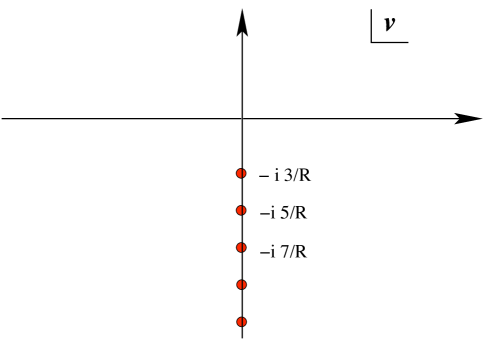
Figure 5.2: The analytic structure in complex frequency plane, of the massless, spatially homogeneous ($l=n=0$), retarded Green’s function in the ${\mathbb{Z}}_{N}$ symmetric phase, corresponding to the topological AdS black hole.

The divergent and scheme-dependent contact terms can be minimally subtracted away to yield the renormalized, retarded Green’s function. Up to now, we have been working with dimensionless variables, corresponding to a de Sitter boundary of unit curvature. Restoring dimensionful constants with the replacement

$$\nu\rightarrow\nu R_{\rm dS},$$ (5.26)

$R_{\rm dS}$ being the radius of curvature of the boundary $dS_{3}$ or the inverse Hubble constant , the renormalized retarded Green’s function continued into the complex frequency plane is given by

$$\tilde{G}_{R_{\rm dS}}(\nu;0)=-\frac{N^{2}}{64\pi^{2}}(R_{\rm dS}^{-2}+\nu^{2})^{2}\;\left[\psi\left({3-i\nu R_{\rm dS}\over 2}\right)-{2i\nu R_{\rm dS}\over(1+\nu^{2}R_{\rm dS}^{2})}\right].$$ (5.27)

For ${\rm Im}(\nu)=0$, its real and imaginary parts match (5.25) and the function is analytic in the upper half plane, with only isolated simple poles in the lower half plane at

$$\nu_{k}=-i(3+2k){1\over R_{\rm dS}},\qquad{\rm with}\qquad k\in{\mathbb{Z}}.$$ (5.28)

This is depicted in Fig. 5.2.

As argued in Son:2002sd , poles of the retarded correlator in a black hole background coincide with the quasinormal frequencies of the black hole. The quasinormal frequencies and the retarded glueball correlator found for the topological black hole in $AdS_{5}$ are remarkably similar to the corresponding objects in the BTZ black hole Son:2002sd .

5.1.2.2 Non-zero Momentum along $S^{1}$ and $\ell=0$

It is relatively easy to allow for a non-zero discrete momentum $n/r_{\chi}$ along the spatial $S^{1}$. To solve the boundary value problem in the topological black hole background, this requires the modes (LABEL:massless). Following the same steps as in the $s$-wave correlator, we find that the retarded Green’s function is

$$\tilde{G}_{R}(\nu\,;n) = -\frac{N^{2}}{128\pi^{2}}\left((\nu-\tfrac{n}{r_{\chi}})^{2}+R_{\rm dS}^{-2}\right)\left((\nu+\tfrac{n}{r_{\chi}})^{2}+R_{\rm dS}^{-2}\right)\,\times$$

$$\left[\psi\left(\frac{3}{2}-i\tfrac{R_{\rm dS}}{2}(\nu-\tfrac{n}{r_{\chi}})\right)+\psi\left(\frac{3}{2}-i\tfrac{R_{\rm dS}}{2}(\nu+\tfrac{n}{r_{\chi}})\right)-{2iR(\nu-\tfrac{n}{r_{\chi}})\over(\nu-\tfrac{n}{r_{\chi}})^{2}R_{\rm dS}^{2}+1}-{2iR_{\rm dS}(\nu+\tfrac{n}{r_{\chi}})\over(\nu+\tfrac{n}{r_{\chi}})^{2}R_{\rm dS}^{2}+1}\right]\,,$$

$$n\in{\mathbb{Z}}.$$

Here, we have restored the dimensionful constants. When $n=0$, this matches our expression for the $s$-wave correlator (5.27).

The Green’s function has nonanalyticities only in the lower half plane, with simple poles at

$$\nu_{k}^{\pm}=-i(3+2k)R_{\rm dS}^{-1}\pm{n\over r_{\chi}};\qquad k,n\in{\mathbb{Z}},$$ (5.30)

giving the quasinormal frequencies of the topological black hole, with non-zero momentum along the spatial $S^{1}$. Interestingly, each simple pole at $n=0$ “splits” into two simple poles at non-zero $n$ (see Fig. 5.3).

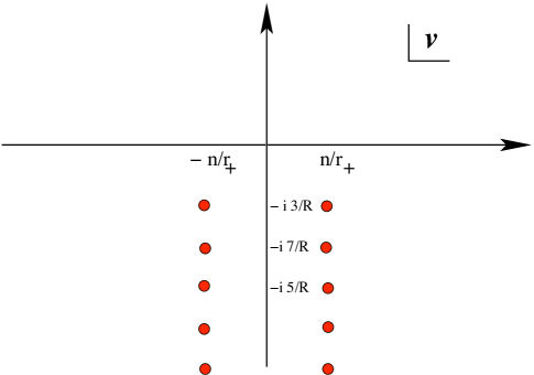
Figure 5.3: Simple poles in the frequency plane, of the massless retarded Green’s function with non-zero momentum along the spatial circle.

We would like to also note that our expressions for the correlation functions on $dS_{3}\times S^{1}$ in the ${\mathbb{Z}}_{N}$ symmetric phase satisfy the obvious consistency check: in the high frequency/large momentum limit $\nu R,n\gg 1$, they reproduce the flat space Green’s function for the scalar glueball operator

$$\tilde{G}_{R}(\nu\,;n)\Big{|}_{\nu R,\,n\gg 1}\longrightarrow-{N^{2}\over 128\pi^{2}}(\nu^{2}-\tfrac{n^{2}}{r_{\chi}^{2}})^{2}\;\ln(\nu^{2}-\tfrac{n^{2}}{r_{\chi}^{2}}).$$ (5.31)

5.1.3 Thermal Effects and the Gibbons-Hawking Temperature

The de Sitter space has a cosmological horizon and an associated Gibbons-Hawking temperature Gibbons:1977mu . We therefore expect our boundary ($dS_{3}\times S^{1}$) field theory correlators to exhibit thermal properties. For real frequencies $\nu$, the digamma functions have an imaginary part so that

$$\begin{split}{\rm Im}\;\tilde{G}_{R}(\nu\,;n)\Big{|}_{{\rm Im}(\nu)=0}=&\,{N^{2}\over 256\pi}\left((\nu-\tfrac{n}{r_{\chi}})^{2}+R^{-2}\right)\left((\nu+\tfrac{n}{r_{\chi}})^{2}+R^{-2}\right)\times\\ &\left[\coth\left(\frac{\pi R}{2}(\nu+\tfrac{n}{r_{\chi}}-iR^{-1})\right)+\coth\left(\frac{\pi R}{2}(\nu+\tfrac{n}{r_{\chi}}-iR^{-1})\right)\right].\end{split}$$ (5.32)

Here we have used $\tanh(x)=\coth(x+i\tfrac{\pi}{2})$ to cast the result in a form that will make the connection to thermal physics explicit.

In flat space and in free field theory at finite temperature $T\neq 0$, the scalar glueball propagator with zero spatial momentum and frequency $\omega$ is proportional to the digamma function Hartnoll:2005ju

$$\tilde{G}_{R}(\omega)\big{|}_{\rm Flat\;space}=-{N^{2}\over 2\pi^{2}}\;\omega^{4}\psi\left(-i\omega\over 4\pi T\right)+{\rm analytic}.$$ (5.33)

The imaginary part of the flat space glueball correlator is given by the spectral function

$${\rm Im}\;\tilde{G}_{R}(\omega)\big{|}_{\rm Flat\;space}=-{N^{2}\over 2\pi^{2}}\omega^{4}\pi\coth\left({\omega\over 4T}\right).$$ (5.34)

In weakly coupled, or free field theories at finite temperature on flat space, the one-loop spectral function reflects the physical effect of “Bose enhancement”, which follows from the stimulated emission of bosons into the heat bath. In perturbative field theory on flat space, this manifests itself as an enhancement of the decay rate of an unstable boson in a heat bath by a factor (relative to the vacuum decay rate)

$$\coth\left({\omega\over 4T}\right)=1+2n_{B}\left(\tfrac{\omega}{2}\right)=1+{2\over e^{\omega/2T}-1}.$$ (5.35)

Here, we have assumed that the unstable boson is at rest with energy $\omega$.

While there may not be an obvious way to define a spectral representation in de Sitter space, the similarity between our strongly coupled de Sitter space result (5.32) and (5.34) is obvious. In particular, it allows the identification of a temperature in de Sitter space

$$T_{H}={R_{\rm dS}^{-1}\over 2\pi}$$ (5.36)

which is precisely the value of the Gibbons-Hawking temperature.

We note that despite the similarity between the expressions for $dS_{3}$ and thermal correlators in flat space, there is a crucial difference – the frequency or energy appearing in the Bose-Einstein-like distribution function in de Sitter space, is not the real frequency $\nu$ (5.32), but in fact $\nu-iR_{\rm dS}^{-1}$. This difference can be traced back to the definition of our positive and negative frequency modes (6.9). For real $\nu$, the positive frequency modes are red-shifted away in the far future. To get propagating modes in the future, we would need to choose $\nu=\omega+iR_{\rm dS}^{-1}$ with $\omega\in{\mathbb{R}}$.

It has been argued in Kovtun:2007py ; Unsal:2008ch that correlation functions of large $N$ gauge theories in the ${\mathbb{Z}}_{N}$ symmetric phase, with some or all spacetime directions compactified, should be independent of the volume of the compact directions. In the present situation, this would imply that on $dS_{3}\times S^{1}$ with antiperiodic boundary conditions for the fermions, large $N$ correlators in the ${\mathbb{Z}}_{N}$ symmetric phase ($r_{\chi}>R_{\rm AdS}/2\sqrt{2}$) should be independent of the radius of the $S^{1}$. In particular then, for perturbations which are homogeneous along the circle, the correlation functions should be independent of $r_{\chi}$ and should match up with the result on $dS_{3}\times{\mathbb{R}}$. The latter is obtained by a (double) Wick rotation of $S^{3}\times{\mathbb{R}}$. Since ${\rm Tr}F^{2}$ is a chiral primary in the ${\cal N}=4$ theory and its correlator on $S^{3}\times{\mathbb{R}}$ is not renormalized by interactions, one would expect this to be true also on $dS_{3}\times{\mathbb{R}}$. We would like to emphasize that this expectation is only for correlators evaluated on the vacuum obtained by analytic continuation. Therefore, we should not expect that the correlators in a general $\alpha$-vacuum to be renormalized. In particular, the transition amplitudes between two different vacua will not be renormalized: in free or weakly coupled theory, they are identical to zero, but our results from Chapter 7 seem to suggest that they are not zero in the strong coupling regime.

5.1.4 The Massive Case

The holographic calculation of correlation functions in the topological AdS black hole can be easily extended to the case of massive scalars. In the context of the Type IIB theory, such massive states are stringy excitations with masses $M^{2}\sim\alpha^{\prime-1}\gg R^{-2}_{\rm AdS}$. A scalar field of mass $M$ in the bulk is dual to a scalar operator ${\cal O}_{\Delta}$ in the field theory with conformal dimension $\Delta=2+\sqrt{4+(MR_{\rm AdS})^{2}}$. We will study below the free massive scalar in the bulk geometry to extract information on the analytic structure of correlators of high dimension operators in the field theory.

There are two primary motivations for looking at high dimension operators in the field theory:

• i) The works of Fidkowski:2003nf ; Festuccia:2005pi have demonstrated that propagators of heavy fields, in the geodesic approximation, may be used to probe the bulk geometry behind horizons and perhaps extract information on singularities behind such horizons.

• ii) One of our main goals is to look for signatures of the transition between a ${\mathbb{Z}}_{N}$ symmetric phase and a ${\mathbb{Z}}_{N}$ broken phase. In the bulk theory, the latter phase is the small bubble of nothing geometry. Correlators in this latter geometry can only be computed using an eikonal (WKB) approximation involving high frequencies and/or large masses.

Extending the holographic analysis done above for massless fields, to massive scalars in the topological black hole geometry, we find that the frequency space correlator is

$$\tilde{G}_{R}(\nu)={\cal C}_{\Delta}\;{\Gamma\left(\tfrac{1}{2}\left(\Delta-1-i\nu R_{\rm dS}\right)\right)^{2}\Gamma\left(3-\Delta\right)\over\Gamma\left(\tfrac{1}{2}\left(3-\Delta-i\nu R_{\rm dS}\right)\right)^{2}\Gamma(\Delta-1)},$$ (5.37)

where the normalization constant ${\cal C}_{\Delta}=2(\Delta-2)\epsilon^{2(\Delta-4)}$, with $\epsilon\rightarrow 0$ as the boundary is approached.

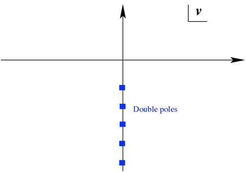
Figure 5.4: Double poles in the lower half plane for the massive (retarded) propagator at zero spatial momentum.

In the massless limit $MR_{\rm AdS}\rightarrow 0$, after subtracting an additional divergent contact term, this reproduces the expression (5.27) found previously. The massive correlator has an analytic structure that is qualitatively distinct from the massless case. In particular, the retarded correlator has an infinite set of double poles and simple poles at

$$\nu_{k}=-i(\Delta-1+2k){1\over R_{\rm dS}}\,,\qquad k\in{\mathbb{Z}}.$$ (5.38)

See Fig. 5.4.

The significance of the appearance of double poles in the massive retarded propagator is not entirely clear. Such double poles have also appeared in 2d CFT correlators with non-integer conformal dimensions from the BTZ black hole Son:2002sd , at zero spatial momentum. At finite spatial momentum, i.e., $n\neq 0$, we expect the double poles to split into simple poles.

For real frequencies, the massive correlator also has an imaginary part

$${\rm Im}\;\tilde{G}_{R}(\nu)=-\tfrac{\pi^{2}}{2}{\cal C}_{\Delta}{\Gamma(3-\Delta)\over\Gamma(\Delta-1)}\;{\sin\left(\pi\,\Delta\right)\;\sinh\left(\pi\;\nu R_{\rm dS}\right)\over|\Gamma\left(\tfrac{1}{2}(3-\Delta-i\nu R_{\rm dS})\right)\cos\left(\tfrac{\pi}{2}(\Delta-i\nu R_{\rm dS})\right)|^{4}}.$$ (5.39)

The de Sitter thermal origin of this result is not as explicit as for the massless scalar. However, after identifying the de Sitter Hawking temperature to be $T_{H}=R_{\rm dS}^{-1}/2\pi$, it is worth comparing the above expression with the imaginary part of the propagator in two dimensions for large non-integer conformal dimension deduced from the non-extremal BTZ black hole Son:2002sd . The similarities between the two results, particularly the numerator of (5.39), are striking.

The large mass, high frequency limit of this result is easily obtained, using Stirling’s approximation

$$\Gamma(z)\big{|}_{z\gg 1}\simeq\sqrt{2\pi}{1\over\sqrt{z}}\;e^{-z}\;z^{z}.$$ (5.40)

When the masses are taken to be large so that $MR_{\rm AdS}\gg 1$, then $\Delta\approx MR_{\rm AdS}$. In this high frequency and large mass limit, it is useful to define a rescaled frequency variable

$$\tilde{\nu}\equiv{\nu\over M},\qquad\nu R_{\rm dS},\;MR_{\rm AdS}\gg 1,$$ (5.41)

so that

$$G_{R}(\tilde{\nu})\sim{\cal C}_{\Delta}\left({1-i\tilde{\nu}\over 2}\right)^{MR_{\rm dS}(1-i\tilde{\nu})}\;\left({-1-i\tilde{\nu}\over 2}\right)^{MR_{\rm dS}(1+i\tilde{\nu})}.$$ (5.42)

Here, we have ignored an overall (real) phase due to the frequency independent coefficients in the large mass limit. At first sight, a potentially problematic feature of this approximation appears. It seems that there is a branch point singularity at $\tilde{\nu}=+i$ which would imply a non-analyticity in the upper half plane, inconsistent with the definition of a retarded propagator. We note that this feature is purely a result of the high frequency approximation and the exact result (5.37) has no singularities in the upper half of the complex frequency plane. Indeed, closer inspection reveals that the putative branch cut originating at $\tilde{\nu}=+i$ has a vanishing discontinuity in the limit of large $MR_{\rm AdS}$. The spurious branch cut originates from the equally spaced zeroes of $G_{R}(\nu)$ appearing to coalesce in the high frequency limit. The branch cut discontinuity at $\tilde{\nu}=-i$ is, however, a genuine non-analyticity and originates from the infinite set of poles merging into a continuum in the high frequency approximation. See Fig. 5.5

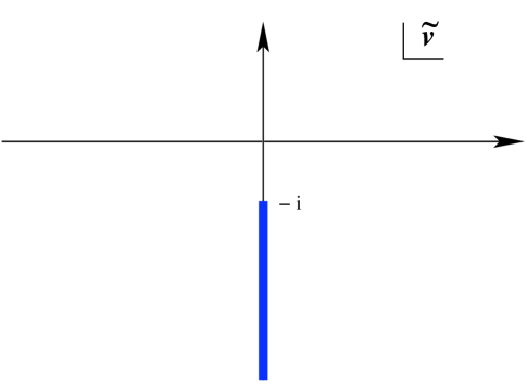
Figure 5.5: For large mass and frequency, the propagator in the topological black hole phase, has a branch cut as indicated in the rescaled frequency plane, $\tilde{\nu}=\nu/M$. This results from the apparent merging of the infinite set of isolated poles of the exact Green’s function.

The easiest way to understand the singularities and discontinuities of the function above is by examining the function $z^{2MR_{\rm dS}z}\;(z-1)^{-2MR_{\rm dS}(z-1)}$ and then make the replacement $z\rightarrow(1-i\tilde{\nu})/2$.

Along the branch cut ${\cal B}\equiv\left\{\tilde{\nu}\in[-i,-i\infty)\right\}$, we find that the retarded propagator has a discontinuity

$$\begin{split}{\rm Disc}|_{\cal B}\;\tilde{G}_{R}(M\tilde{\nu})=&2i\;{\cal C}_{\Delta}\;\sin(2\pi MR_{\rm dS})\left({|\tilde{\nu}|+1\over 2}\right)^{MR_{\rm dS}(|\tilde{\nu}|+1)}\left({|\tilde{\nu}|-1\over 2}\right)^{-MR_{\rm dS}(|\tilde{\nu}|-1)}\,,\\ &\tilde{\nu}=-i|\tilde{\nu}|\,,\quad|\tilde{\nu}|\geq 1.\end{split}$$ (5.43)

It is clear that the discontinuity is large in the large mass limit.

Now, let us look closely at the putative branch cut along the imaginary axis ${\cal B}^{\prime}\equiv\left\{\tilde{\nu}\in[-i,i]\right\}$. Computing the discontinuity across this, we have

$$\begin{split}{\rm Disc}|_{{\cal B}^{\prime}}\;\tilde{G}_{R}(M\tilde{\nu})&=\,2i\;{\cal C}_{\Delta}\sin\left(MR_{\rm dS}\pi(1-x)\right)\left({1+x\over 2}\right)^{MR_{\rm dS}(1+x)}\left({1-x\over 2}\right)^{MR_{\rm dS}(1-x)},\\ &\tilde{\nu}=ix,\,\quad-1\leq x\leq 1.\end{split}$$ (5.44)

This vanishes when $MR_{\rm dS}\rightarrow\infty$, for two reasons: the rapid sinusoidal oscillations will give vanishing contribution to any contour integral along ${\cal B}^{\prime}$ and furthermore, the amplitude of the oscillations vanishes exponentially as evident from the expression above.

In the leading high frequency approximation , for real frequencies, the imaginary and real parts of the Green’s function are given by

$$\begin{split}\tilde{G}_{R}(\nu)&\approx{\cal C}_{\Delta}\;\left({\nu^{2}+M^{2}\over 4M^{2}}\right)^{MR_{\rm dS}}e^{-\tfrac{1}{\pi}\tfrac{\nu}{T_{H}}\tan^{-1}\tfrac{\nu}{M}}\;e^{-\tfrac{|\nu|}{2T_{H}}}\left(\cos(\tfrac{M}{2T_{H}})-i\;{\rm sgn}(\nu)\sin(\tfrac{M}{2T_{H}})\right),\\ &\qquad T_{H}={R_{\rm dS}^{-1}\over 2\pi}\,,\quad\nu\in{\mathbb{R}}.\end{split}$$ (5.45)

The high frequency, large mass limit thus appears to retain features of the thermal effects of de Sitter space. This result can be deduced from (5.42) after choosing an appropriate branch of the function and also directly follows from (5.39). We will see subsequently that these high frequency expressions can also be derived by solving the wave equations using a WKB approximation, providing a consistency check.

5.2 WKB for the AdS Bubble of Nothing

An exact holographic computation of correlation functions in the AdS bubble of nothing background appears difficult as analytical solutions to the wave equation in this background are not known. Despite this, we may obtain the boundary Green’s function following a systematic approximation. In particular, we will employ the WKB approximation to determine boundary correlation functions at high frequency and large mass. The WKB approximation has been used successfully to find high frequency Green’s functions in the Big AdS-Schwarzschild black hole Festuccia:2005pi . In this approximation, lines of isolated singularities (poles) get replaced by branch cuts since in the high frequency regime, the separation between poles effectively goes to zero, as seen in our example above in Section 5.1.4.

We first take the massive scalar wave equation

$${1\over\sqrt{-g}}\;\partial_{\mu}(g^{\mu\nu}\sqrt{-g}\;\partial_{\nu}\Phi)-M^{2}\Phi=0,$$ (5.46)

in the bubble background and expand the scalar field in harmonics on $dS_{3}\times S^{1}$ as in (5.3). The harmonics $\Phi_{n}(\nu,\rho)$ then satisfy a radial differential equation which can be put in the form

$$\begin{split}{1\over 4(x-1)(x+\tilde{r}_{h}^{2})(x-\tilde{r}_{h}^{2}-1)}\left({\nu^{2}+1}-{n^{2}}{R^{2}_{\rm AdS}\over r_{\chi}^{2}}{(x-1)^{2}\over(x+\tilde{r}_{h}^{2})(x-\tilde{r}_{h}^{2}-1)}-{M^{2}R_{\rm AdS}^{2}}(x-1)\right)\Phi_{n}&\\ \\ +{d^{2}\Phi_{n}\over dx^{2}}+\left({1\over x-1}+{1\over x+\tilde{r}_{h}^{2}}+{1\over x-\tilde{r}_{h}^{2}-1}\right){d\Phi_{n}\over dx}&=0,\end{split}$$ (5.47)

where $x=\rho^{2}$ and $n$ labels the momentum along the $S^{1}$.

This is an ordinary differential equation with four regular or nonessential singular points at $x=1,\,-\tilde{r}_{h}^{2},\,\tilde{r}_{h}^{2}+1$ and $\infty$. Analytical solutions for this type of equation are unknown. In fact, a similar differential equation was encountered in the computation of glueball masses at strong coupling in the three dimensional effective theory obtained from thermal ${\cal N}=4$ SYM Csaki:1998qr on ${\mathbb{R}^{3}}\times S^{1}$ with SUSY-breaking boundary conditions. In that case, the dual bulk geometry is the Euclidean black brane solution in AdS space where the thermal circle shrinks to zero size smoothly.

It will be convenient to rewrite the differential equation in the Schrödinger form by introducing the variables

$$\Phi={\Psi\over\sqrt{\rho(\rho^{2}-1)}},$$ (5.48)

$$u\;=\;{\tilde{r}_{h}\over 1+2\tilde{r}_{h}^{2}}\;\cot^{-1}\left({\rho\over\tilde{r}_{h}}\right)+{\sqrt{1+\tilde{r}_{h}^{2}}\over{1+2\tilde{r}_{h}^{2}}}\;\coth^{-1}\left({\rho\over\sqrt{1+\tilde{r}_{h}^{2}}}\right).$$ (5.49)

These are the natural generalizations of (5.6) and (5.7) to the bubble of nothing geometry. The cigar in the geometry gets smoothly capped off at $\rho=\sqrt{\tilde{r}_{h}^{2}+1}$, where the spacetime ends. In terms of the $u$ coordinate, this occurs as $u\rightarrow\infty$. In terms of the harmonics of $\Psi$ on the $dS^{3}\times S^{1}$ slices, as in (5.3), we obtain the Schrödinger equation obeyed by the harmonics $\Psi_{n}(\nu,u)$ in the small AdS bubble of nothing. It is given by

$$-{d^{2}\over du^{2}}\;\Psi_{n}(\nu,u)+\tilde{V}_{n}(\nu,u)\;\Psi_{n}(\nu,u)=0,$$ (5.50)

with the potential

$$\tilde{V}_{n}(\nu,u) = \left((MR_{\rm AdS})^{2}-{\nu^{2}+1\over\rho^{2}-1}\right)\left(\rho^{2}-1-{1\over\rho^{2}}\;\tilde{r}_{h}^{2}\;(\tilde{r}_{h}^{2}+1)\right)$$ (5.51)

$$+\,n^{2}\,{R^{2}_{\rm AdS}\over r_{\chi}^{2}}\;{\rho^{2}-1\over\rho^{2}}+{1\over 4\rho^{2}}\;(15\rho^{4}-10\rho^{2}-1).$$

Here, $\rho$ is implicitly a function of $u$, determined by the solution to (5.49). In addition to the fact that the Schrödinger potential is far more complicated than (5.9), one crucial difference to the case of the topological black hole is that the potential cannot be defined independent of the frequency itself. This is due to the term proportional to $\tilde{r}_{h}$ in Eq. (5.51). This situation is also in contrast to the case of the big AdS-Schwarzschild black hole in Festuccia:2005pi . Here, for a given frequency and mass, we need to find the “zero energy” eigenstate of the Schrödinger problem (5.50).

Interestingly, the qualitative behaviour of the potential $\tilde{V}_{n}$ changes, depending on the relative values of the mass and the frequency. This is illustrated in Figures (5.6) and (5.7).

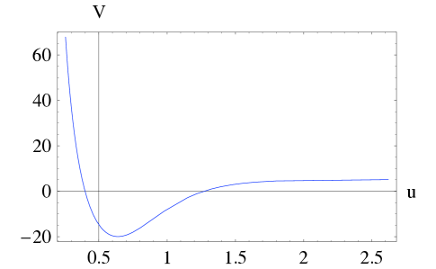
Figure 5.6: The Schrödinger potential for a massive scalar in the AdS bubble of nothing. In the above plot the dimensionless frequency $\nu=7$, the mass $MR_{\rm AdS}=2$ and $\tilde{r}_{h}=r_{h}/R_{\rm AdS}=1$.

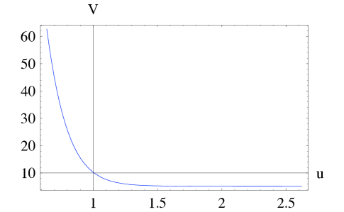
Figure 5.7: The Schrödinger potential for $\nu=7$, the mass $MR=7$ and $\tilde{r}_{h}=r_{h}/R_{\rm AdS}=1$.

The qualitative nature of the potential is easy to grasp in the high frequency limit, wherein we take

$$\nu\rightarrow\infty\qquad{\rm and}\qquad MR_{\rm AdS}\rightarrow\infty,$$ (5.52)

while keeping

$$\tilde{\nu}={\nu\over MR_{\rm AdS}}$$ (5.53)

fixed. For simplicity, we also set $n=0$, focussing attention on the spatially homogeneous fields. In this approximation, the potential $\tilde{V}_{0}(\nu,u)$ becomes

$${\cal V}(\tilde{\nu},u)=(MR_{\rm AdS})^{2}\left(1-{\tilde{\nu}^{2}\over\rho^{2}-1}\right)\left(\rho^{2}-1-{1\over\rho^{2}}\;\tilde{r}_{h}^{2}(\tilde{r}_{h}^{2}+1)\right).$$ (5.54)

Having thrown away a subleading constant in the large frequency limit, the potential is vanishing at the tip of the cigar $\rho=\sqrt{\tilde{r}_{h}^{2}+1}$. Using $u\sim-\ln(\rho-\sqrt{\tilde{r}_{h}^{2}+1})$ near this point, it follows that ${\cal V}(\tilde{\nu},u)$ decays exponentially as a function of $u$.

The potential has another zero at $\rho=\sqrt{{\tilde{\nu}}^{2}+1}$. Now, since the spacetime ends at $\rho=\sqrt{1+\tilde{r}_{h}^{2}}$, the number of zeroes of the potential depends on whether $|\tilde{\nu}|$ is greater than or less than $\tilde{r}_{h}$. In particular, when $|\tilde{\nu}|>\tilde{r}_{h}$, the potential energy has two zeroes or turning points, and qualitatively resembles Fig. 5.6, while for $|\tilde{\nu}|<\tilde{r}_{h}$, it behaves as in Fig. (5.7). In the latter case, the potential asymptotes to a constant different from zero in the figures, however, this constant becomes negligible in the high frequency limit.

Zero energy Schrödinger wave functions in the potential (5.54) are marginally bound states for $|\tilde{\nu}|>\tilde{r}_{h}$, since the potential has two turning points. For $|\tilde{\nu}|<\tilde{r}_{h}$, there is only one turning point and the wave function should exhibit a qualitative change in its behaviour at $|\tilde{\nu}|=\tilde{r}_{h}$. This also strongly suggests that in the complex frequency plane, $\tilde{\nu}=\pm\tilde{r}_{h}$ should be singularities of boundary correlation functions.

The zero energy wave function for the Schrödinger equation can be obtained in the WKB approximation, where care needs to be taken in applying the matching conditions at each of the turning points in the potential. We treat the two cases $|\tilde{\nu}|>\tilde{r}_{h}$ and $|\tilde{\nu}|<\tilde{r}_{h}$ separately.

5.2.1 WKB Approximation for $\nu>\tilde{r}_{h}$

There are two distinct regions in the potential:

• the “quantum tunnelling region”, which corresponds to the regime

  $$\sqrt{1+\tilde{\nu}^{2}}<\rho<\infty,$$ (5.55)

  which we label as Region I;

• the “propagating region”, which corresponds to the regime

  $$\sqrt{1+\tilde{r}_{h}^{2}}<\rho<\sqrt{1+\tilde{\nu}^{2}},$$ (5.56)

  which we will call Region II.

In Region I, we write the WKB solutions as

$$\Psi_{\rm WKB}(\tilde{\nu},u)=\;{1\over{\cal V}^{1/4}}\;\left(A_{+}\exp\left({\int_{u_{c}}^{u}\sqrt{\cal V}\;du}\right)+A_{-}\;\exp\left({-\int_{u_{c}}^{u}\sqrt{\cal V}\;du}\right)\right),$$ (5.57)

where the classical turning point $u_{c}$ is defined by

$$\rho(u_{c})\equiv\sqrt{\tilde{\nu}^{2}+1}.$$ (5.58)

These represent the growing and decaying modes in the near boundary region of the bulk geometry. This can be understood easily as follows. Since

$${du\over d\rho}\bigg{|}_{\rho\to\infty}\approx-{1\over\rho^{2}}$$ (5.59)

in this regime, we have

$${\cal V}\approx(MR_{\rm AdS})^{2}\;\rho^{2},$$ (5.60)

which then immediately yields the near boundary WKB solution (5.57) for $\Psi$. This, together with its relation (5.49) to the massive bulk scalar field $\Phi$, implies that

$$\Phi_{\rm WKB}\big{|}_{\rm\rho\rightarrow\infty}\sim A_{+}\;(\cdots)\rho^{-2-MR_{\rm AdS}}+A_{-}\;(\cdots)\;\rho^{-2+MR_{\rm AdS}},$$ (5.61)

where the ellipses denote unspecified normalization constants. The two power laws appearing in this solution are precisely the normalizable and non-normalizable modes of the massive scalar field, in the limit of large mass, in an asymptotically locally AdS spacetime. Following the prescription for computing the retarded Green’s functions, we normalize $\Psi_{\rm WKB}$ (5.61) so that it approaches unity near the boundary.

In the interior, however, for $\rho\leq\sqrt{1+\tilde{\nu}^{2}}$ the solutions enter Region II and become oscillatory. In Region II, we have

$$\Psi_{\rm WKB}(\tilde{\nu},u)=\;{1\over|{\cal V}|^{1/4}}\left(B_{+}\;\exp\left(i{\int_{u_{c}}^{u}\sqrt{|{\cal V}|}\;d\rho}\right)+B_{-}\;\exp\left({-i\int_{u_{c}}^{u}\sqrt{|{\cal V}|}\;du}\right)\right).$$ (5.62)

The constants are uniquely determined by the WKB matching conditions at the classical turning points of the potential ${\cal V}(\tilde{\nu},u)$ and the one normalization condition on $A_{-}$ near the boundary.

Near the turning point $u=u_{c}$ corresponding to $\rho=\sqrt{1+\nu^{2}}$, since we are well away from any extrema, we can assume that

$${\cal V}(\nu,u)=\kappa(u_{c}-u)+\ldots\,,\qquad{u\to u_{c}}.$$ (5.63)

In this region, where the potential is basically linear, the exact solution in terms of Airy functions is given by

$$\Psi\big{|}_{u\to u_{c}}=A_{+}\;{2\sqrt{\pi}\over\kappa^{1/6}}\;{\rm Ai}\left(\kappa^{1/3}(u_{c}-u)\right)+A_{-}\;{\sqrt{\pi}\over\kappa^{1/6}}\;{\rm Bi}\left(\kappa^{1/3}(u_{c}-u)\right).$$ (5.64)

The normalizations and constants of integration have been chosen carefully so that near the turning point, the exact solution, which is given in terms of the Airy functions, matches the WKB solution (5.57) in Region I ($u<u_{c}$) away from the turning point.

Now, we can continue the solution (5.64) into Region II ($u>u_{c}$). For $u>u_{c}$, where the WKB solution (5.62) should be valid, the Airy functions have the asymptotic form

$$\Psi\big{|}_{u>u_{c}}\approx 2A_{+}\;{\sin\left(\tfrac{2}{3}\sqrt{\kappa}(u-u_{c})^{3/2}+\tfrac{\pi}{4}\right)\over\kappa^{1/4}(u-u_{c})^{1/4}}+A_{-}\;{\cos\left(\tfrac{2}{3}\sqrt{\kappa}(u-u_{c})^{3/2}+\tfrac{\pi}{4}\right)\over\kappa^{1/4}(u-u_{c})^{1/4}}.$$ (5.65)

Comparison with (5.62) near the turning point then implies

$$B_{+}=e^{i\tfrac{\pi}{4}}\left(\tfrac{1}{2}A_{-}-iA_{+}\right)\,,\qquad{\rm and}\qquad B_{-}=e^{-i\tfrac{\pi}{4}}\left(\tfrac{1}{2}A_{-}+iA_{+}\right).$$ (5.66)

There is yet another condition that emerges from the behaviour of the solutions near the second “turning point”, $\rho\rightarrow\sqrt{1+\tilde{r}_{h}^{2}}$ or $u\rightarrow\infty$ where the space ends. In this region, we have

$${du\over d\rho}\big{|}_{\rho\to\sqrt{1+\tilde{r}_{h}^{2}}}\approx-{\sqrt{1+\tilde{r}_{h}^{2}}\over 2(2\tilde{r}_{h}^{2}+1)(\rho-\sqrt{1+\tilde{r}_{h}^{2}})}$$ (5.67)

so that

$$\rho-\sqrt{1+\tilde{r}_{h}^{2}}\;\approx\;2\sqrt{1+\tilde{r}_{h}^{2}}\exp\left(-2\tfrac{(1+2\tilde{r}_{h}^{2})}{\sqrt{1+\tilde{r}_{h}^{2}}}\;u+\tfrac{\tilde{r}_{h}}{\sqrt{1+\tilde{r}_{h}^{2}}}\cot^{-1}\left(\tfrac{\sqrt{1+\tilde{r}_{h}^{2}}}{\tilde{r}_{h}}\right)\right).$$ (5.68)

It follows then that, as a function of $u$, the high frequency potential decays exponentially,

$${\cal V}(\nu,u)\big{|}_{u\rightarrow\infty}\approx(MR_{\rm AdS})^{2}\left(1-{\nu^{2}\over\tilde{r}_{h}^{2}}\right)\;\exp\left(-2\tfrac{(1+2\tilde{r}_{h}^{2})}{\sqrt{1+\tilde{r}_{h}^{2}}}\;u+{\rm constants}\right).$$ (5.69)

We note that for $\nu>\tilde{r}_{h}$, this potential approaches zero from below. Let us define constants $A$ and $B$, in terms of which the potential is simply

$$\tilde{V}_{0}(\nu,u)\big{|}_{u\rightarrow\infty}\approx-Ae^{-Bu},$$ (5.70)

where $A$ and $B$ can be read off easily from the expressions above.

The Schrödinger equation with an exponentially decaying potential

$$-\Psi^{\prime\prime}(u)-Ae^{-Bu}\Psi(u)=0$$ (5.71)

is solved exactly by Bessel functions

$$\Psi=C_{1}\;J_{0}\left(2\tfrac{\sqrt{A}}{B}\,e^{-Bu/2}\right)+C_{2}\;Y_{0}\left(2\tfrac{\sqrt{A}}{B}\,e^{-Bu/2}\right).$$ (5.72)

Since we are looking for a zero energy eigenfunction of the Schrödinger problem, this means that for a potential that vanishes at infinity, the corresponding (normalizable) wavefunction can only be zero. This is an important difference to the black hole case where the wave functions are infalling plane waves at the horizon. In the bubble geometry, however, since spacetime ends smoothly in the interior where the cigar caps off, there is no freedom in choosing the boundary condition at the tip of the cigar – we must require regularity (normalizability) of solutions in the interior. This means that the solution to the Schrödinger equation (5.50) must approach a constant exponentially as $u\to\infty$.

Requiring that the wave function $\Psi$ vanish or approach a constant as $u\to\infty$ then eliminates the term proportional to $Y_{0}$. Hence, in the exponentially decaying region

$$\Psi(u)\propto J_{0}\left(2\tfrac{\sqrt{A}}{B}\,e^{-Bu/2}\right).$$ (5.73)

The WKB approximation should then match onto the Bessel function for large values of the argument of the Bessel function. Using the standard asymptotic expansion for Bessel functions

$$J_{0}(x)\big{|}_{x\gg 1}\simeq{\cos(x)\over\sqrt{\pi x}}+{\sin(x)\over\sqrt{\pi x}},$$ (5.74)

we can deduce a relationship between the constants $B_{+}$ and $B_{-}$ in (5.62). To make this precise we define the integral

$${\cal S}_{II}(u)=\int^{u}_{\infty}\sqrt{|{\cal V}(\nu,u)|}\;du=-MR_{\rm AdS}\int_{\tilde{r}_{h}}^{\rho^{2}-1}dx\sqrt{x^{2}-\nu^{2}\over{(x^{2}-\tilde{r}_{h}^{2})(x^{2}+1+\tilde{r}_{h}^{2})}},$$ (5.75)

which in radial coordinate $\rho$ is given by

$${\cal S}_{II}(u(\rho)) = i\;\frac{MR_{\rm AdS}}{\sqrt{1+2\tilde{r}_{h}^{2}}}\left[\nu\left(F\left(\sin^{-1}\sqrt{\tfrac{1}{a}\tfrac{\rho^{2}+\tilde{r}_{h}^{2}}{\rho^{2}-1}}\;\bigg{|}\;k\right)-\frac{1}{\sqrt{k}}\;K\left(\tfrac{1}{k}\right)\right)+\right.$$ (5.76)

$$\left.\tfrac{1}{\nu}(1+\tilde{r}_{h}^{2})\left(\Pi\left(a;\,\,\sin^{-1}\sqrt{\tfrac{1}{a}\tfrac{\rho^{2}+\tilde{r}_{h}^{2}}{\rho^{2}-1}}\,\bigg{|}\,k\right)-\frac{1}{\sqrt{k}}\;\Pi\left(b\big{|}\tfrac{1}{k}\right)\right)\right].$$

Here, $F$ and $K$ are the elliptic integrals of the first kind, $\Pi$ is the elliptic integral of the third kind and

$$a=\frac{\nu^{2}+1+\tilde{r}_{h}^{2}}{\nu^{2}}\;,\qquad b=\frac{1+2\tilde{r}_{h}^{2}}{\tilde{r}_{h}^{2}}\;,\qquad k=\frac{a}{b}.$$ (5.77)

Then, the WKB solution in Region II is

$$\Psi_{\rm WKB}={1\over|{\cal V}|^{1/4}}\left(B_{+}\;e^{i{\cal S}_{II}(u)-i{\cal S}_{II}(u_{c})}+B_{-}\,e^{-i{\cal{S}}_{II}(u)+i{\cal S}_{II}(u_{c})}\right).$$ (5.78)

For large $u$,

$${\cal S}_{II}(u)\big{|}_{u\gg 1}\approx\int_{\infty}^{u}\sqrt{A}e^{-Bu/2}=-2{\sqrt{A}\over B}\;e^{-Bu/2}.$$ (5.79)

Using this result and comparing (5.78) to the asymptotics of the Bessel function (5.74), we find

$${B_{+}\over B_{-}}=\;ie^{2i\;{\cal S}_{II}(u_{c})}.$$ (5.80)

The final ingredient consists in determining $A_{+}$ and $A_{-}$. To this end, we first define

$${\cal S}_{I}(u)=\int^{u}_{\infty}\sqrt{{\cal V}(\nu,u)}\;du,$$ (5.81)

which then gives us

$${\cal S}_{I}(u(\rho))=\frac{MR_{\rm AdS}}{\sqrt{1+2\tilde{r}_{h}^{2}}}\left[\nu F\left(\sin^{-1}\left(\sqrt{\tfrac{1}{a}\tfrac{\rho^{2}+\tilde{r}_{h}^{2}}{\rho^{2}-1}}\right),\;k\right)+\tfrac{1}{\nu}(1+\tilde{r}_{h}^{2})\,\Pi\left(a;\sin^{-1}\left(\sqrt{\tfrac{1}{a}\tfrac{\rho^{2}+\tilde{r}_{h}^{2}}{\rho^{2}-1}}\right)\bigg{|}\,k\right)\right],$$ (5.82)

with

$$a=\tfrac{\nu^{2}+1+\tilde{r}_{h}^{2}}{\nu^{2}}\;,\qquad b=\tfrac{1+2\tilde{r}_{h}^{2}}{\tilde{r}_{h}^{2}}\;,\qquad k=\tfrac{a}{b}.$$ (5.83)

Near the boundary $u\to 0$ or equivalently $\rho\to\infty$, we find

$$\begin{split}\Psi_{\rm WKB}\approx&\,A_{-}\tfrac{1}{\sqrt{MR_{\rm AdS}}}\;\rho^{MR_{\rm AdS}-\tfrac{1}{2}}\;e^{i\pi MR_{\rm AdS}/2}\;\left({4\over 1+\tilde{r}_{h}^{2}}\right)^{MR_{\rm AdS}/4}\;\nu^{-MR_{\rm AdS}/2}\,\times\\ &\exp\left[\tfrac{MR_{\rm AdS}}{\sqrt{1+2\tilde{r}_{h}^{2}}}\;\left(\nu(F\left(\csc^{-1}\sqrt{a},\;k\right)-K(k))-\tfrac{1}{\nu}(1+\tilde{r}_{h}^{2})\;\Pi(a|k)\right)\right]\\ &+\;A_{+}\,\tfrac{1}{\sqrt{MR_{\rm AdS}}}\;\rho^{-MR_{\rm AdS}-\tfrac{1}{2}}\;e^{-i\pi MR_{\rm AdS}/2}\;\left({4\over 1+\tilde{r}_{h}^{2}}\right)^{-MR_{\rm AdS}/4}\nu^{MR_{\rm AdS}/2}\,\times\\ &\exp\left[-\tfrac{MR_{\rm AdS}}{\sqrt{1+2\tilde{r}_{h}^{2}}}\;\left(\nu(F\left(\csc^{-1}\sqrt{a},\;k\right)-K(k))-{1\over\nu}(1+\tilde{r}_{h}^{2})\;\Pi(a|k)\right)\right].\end{split}$$ (5.84)

Combining (5.66) and (5.80), we obtain

$$A_{+}=-A_{-}{1\over 2}\;\tan\left({\cal S}_{II}(u_{c})\right).$$ (5.85)

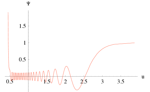
Figure 5.8: The exact numerical solution to the Schrödinger problem for the AdS bubble of nothing. Here, $\nu R_{\rm AdS}=200$, $MR_{\rm AdS}=100$ and $r_{h}/R_{\rm AdS}=1$. The solution approaches a constant for $u\gg 1$, while the classically forbidden region is $0<u<u_{c}\approx 0.49$.

The Green’s function at high frequency is completely determined (up to contact terms) by the ratio $A_{+}/A_{-}$. After substituting the solution (5.61) into the boundary action we find that

$$\tilde{G}_{R}(\tilde{\nu})\approx\lim_{\epsilon\rightarrow 0}\;{MR_{\rm AdS}}\;\exp\left(2\int_{u_{c}}^{\epsilon}\sqrt{{\cal V}(\tilde{\nu},u)}\;du\right)\;\tan\left(\int_{\infty}^{u_{c}}\sqrt{|{\cal V}(\tilde{\nu},u)|}\;du\right).$$ (5.86)

The exponential prefactor in this expression is the WKB transmission coefficient into the classically forbidden Region I. The physically relevant contribution to the transmission coefficient is the constant, $\epsilon$-independent term in an expansion around the boundary $\epsilon\to 0$. The leading $\epsilon$ dependence, which is an overall multiplicative constant proportional to $\epsilon^{2MR_{\rm AdS}}$, can be absorbed into the normalization of the correlation function.

The first observation we can make without actually evaluating (5.86) is that it has an infinite set of poles as a function of $\tilde{\nu}$ on the real axis for $\tilde{\nu}^{2}>r_{h}^{2}$. These occur whenever

$${\cal S}_{II}(\tilde{\nu},\;MR_{\rm AdS})=\int_{\infty}^{u_{c}}du\sqrt{|{\cal V}(\tilde{\nu},u)|}=(n+\tfrac{1}{2}){\pi}\,,\quad n\in{\mathbb{Z}}.$$ (5.87)

That is, the semiclassical action in the propagating region is a half-integral multiple of $\pi$. This is of course the condition for the existence of a bound state wave function and the poles in the Green’s function reflect the appearance of these bound states at certain values of $\tilde{\nu}$ on the real axis. This is unlike the corresponding correlators in the topological black hole phase, which do not have any poles on the real axis.

At first sight, the poles on the real frequency axis might appear somewhat surprising. However, they have the following natural physical interpretation. The low energy physics of the gauge theory on the boundary of the AdS bubble of nothing is that of supersymmetric Yang-Mills theory at large $N$ and strong ’t Hooft coupling on $dS_{3}$. The antiperiodic boundary conditions on the spatial $S^{1}$ make all fermionic excitations massive and the broken supersymmetry leads to large radiative corrections to the scalar masses. In the strongly coupled theory, the dynamical scale of the three dimensional effective theory is expected to be set by $r_{\chi}^{-1}$, the scale of the compact $S^{1}$ direction. When the Gibbons-Hawking temperature $T_{H}=1/(2\pi R)$ in $dS_{3}$ is smaller than $r_{\chi}^{-1}$, we expect the gauge theory to be in a confined phase where the degrees of freedom are gauge singlet glueballs. The appearance of the isolated poles in the high frequency correlators is consistent with this physical picture.

The WKB integral in Region II, in the high frequency approximation to the Green’s function (5.86), can be expressed in terms of complete elliptic integrals as

$$\begin{split}{\cal S}_{II}(\tilde{\nu},\;MR_{\rm AdS})=&\,\tfrac{1}{2}MR_{\rm AdS}\int_{\tilde{\nu}^{2}+1}^{\tilde{r}_{h}^{2}+1}dx\;{\sqrt{\tfrac{\tilde{\nu}^{2}}{x-1}-1}\over\sqrt{(x+\tilde{r}_{h}^{2})(x-\tilde{r}_{h}^{2}-1)}}\\ \\ =&\,i\,\frac{MR_{\rm AdS}}{\sqrt{1+2\tilde{r}_{h}^{2}}}\,\left[|\tilde{\nu}|\left(K(\tfrac{a}{b})-{\sqrt{\tfrac{b}{a}}}\;K\left(\tfrac{b}{a}\right)\right)+\tfrac{1}{|\tilde{\nu}|}(1+\tilde{r}_{h}^{2})\left(\Pi(a\big{|}\tfrac{a}{b})-{\sqrt{\tfrac{b}{a}}}\;\Pi\left(b\big{|}{\tfrac{b}{a}}\right)\right)\right],\end{split}$$ (5.88)

where

$$a=\tfrac{\tilde{\nu}^{2}+1+\tilde{r}_{h}^{2}}{\tilde{\nu}^{2}}\;,\qquad b=\tfrac{1+2\tilde{r}_{h}^{2}}{\tilde{r}_{h}^{2}}\;,\qquad\tilde{\nu}^{2}>r_{h}^{2}.$$ (5.89)

From the general characteristics of these elliptic functions and their singularities elliptic , it can be checked that ${\cal S}_{II}(\tilde{\nu},\;MR_{\rm AdS})$ has no singularities on the real axis for $\tilde{\nu}^{2}>\tilde{r}_{h}^{2}$. Potential logarithmic branch points at $\tilde{\nu}^{2}=\tilde{r}_{h}^{2}$ and at $\tilde{\nu}=0$, cancel out between the individual terms above. In fact, for any fixed value of $\tilde{r}_{h}$, it also follows that, for large $\tilde{\nu}$, the WKB integral increases linearly with $\tilde{\nu}$

$${\cal S}_{II}\propto|\tilde{\nu}|\,,\qquad|\tilde{\nu}|\gg 1.$$ (5.90)

Hence, for $|\tilde{\nu}|\gg\tilde{r}_{h}$, the propagator (5.86) has approximately equally spaced simple poles on the real axis, whenever ${\cal S}_{II}=(n+\tfrac{1}{2})\pi$.

Although there are no other sources of singularities from $S_{II}$, the WKB transmission coefficient in Region I, which also enters the Green’s function (5.86), can have branch point singularities on the real axis

$$\begin{split}{\cal S}_{I}(\tilde{\nu},\;MR_{\rm AdS})&=-\tfrac{1}{2}MR_{\rm AdS}\int_{1+\tilde{\nu}^{2}}^{1/\epsilon^{2}}\;dx\frac{\sqrt{1-\tfrac{\tilde{\nu}^{2}}{x-1}}}{\sqrt{(x+\tilde{r}_{h}^{2})(x-\tilde{r}_{h}^{2}-1)}}\\ \\ &=-\frac{MR_{\rm AdS}}{\sqrt{1+2\tilde{r}_{h}^{2}}}\;\left(|\tilde{\nu}|\left(F\left(\csc^{-1}\sqrt{a},\;\tfrac{a}{b}\right)-K\left(\tfrac{a}{b}\right)\right)-\tfrac{1}{|\tilde{\nu}|}(1+\tilde{r}_{h}^{2})\;\Pi\left(a|\tfrac{a}{b}\right)\right)\\ &\quad-\tfrac{1}{2}MR_{\rm AdS}\left(\ln\left(\tfrac{2\epsilon^{-2}}{|\tilde{\nu}|\sqrt{1+\tilde{r}_{h}^{2}}}\right)+i\pi\right).\end{split}$$ (5.91)

This function is also free of any branch cuts at $\tilde{\nu}=\pm\tilde{r}_{h}$, as can be checked by directly evaluating the integral at this point. However, the logarithmic growth at large $\tilde{\nu}$ implies a branch point at infinity.

As an aside, we would like to mention that the high frequency limit in the topological black hole phase (5.42) can be rederived by formally setting $\tilde{r}_{h}=0$ in the WKB integrals and $\tilde{G}_{R}(\tilde{\nu})\sim\exp({2\,\cal S}_{I})$.

5.2.2 WKB Approximation for $|\nu|<\tilde{r}_{h}$

For low real frequencies $\tilde{\nu}^{2}<\tilde{r}_{h}^{2}$, the nature of the WKB potential changes (see Fig. (5.7)). When $|\nu|<\tilde{r}_{h}$, the potential energy ${\cal V}(\nu,u)$ is a monotonic function of $u$ which exponentially vanishes as $u\rightarrow\infty$. Now, the potential has effectively only one turning point and the wave function has no region where it propagates. The WKB solution (5.57) in Region I should smoothly match onto the exact solution of

$$-\psi^{\prime\prime}(u)+Ae^{-Bu}\psi(u)=0\,,$$ (5.92)

where $A,B>0$. The solutions to these are the modified Bessel’s functions. Enforcing regular behaviour as $u\to\infty$ picks out

$$\psi(u)\propto I_{0}\left(2\tfrac{\sqrt{A}}{B}e^{-Bu/2}\right).$$ (5.93)

The WKB approximation for $I_{0}(x)$ is valid when $x\gg 1$, and here

$$I_{0}(x)\big{|}_{x\gg 1}\simeq{1\over 2\sqrt{2\pi x}}\left(e^{x}+ie^{-x}\right).$$ (5.94)

We write the WKB solution to the wave equation in the bubble of nothing background as

$$\Psi_{\rm WKB}(\nu,u)=A_{+}\,{1\over{\cal V}^{1/4}}\exp\left(\int_{\infty}^{u}\sqrt{{\cal V}}\,du\right)+A_{-}\,{1\over{\cal V}^{1/4}}\exp\left(-\int_{\infty}^{u}\sqrt{{\cal V}}\,du\right).$$ (5.95)

Comparison with the modified Bessel function implies

$$A_{+}=iA_{-}.$$ (5.96)

Near the boundary $u\to 0$, which is equivalent to $\rho\to\infty$, we have

$$\begin{split}\Psi_{\rm WKB}\approx&\,A_{-}\frac{1}{\sqrt{MR_{\rm AdS}}}\;\rho^{MR_{\rm AdS}-\tfrac{1}{2}}\;e^{i\pi MR_{\rm AdS}2}\;\left({4\over 1+\tilde{r}_{h}^{2}}\right)^{MR_{\rm AdS}/4}\;\nu^{-MR_{\rm AdS}/2}\,\times\\ &\exp\left[\tfrac{MR_{\rm AdS}}{\sqrt{1+2\tilde{r}_{h}^{2}}}\;\left(\nu(F\left(\csc^{-1}\sqrt{a},\;k\right)-\tfrac{1}{\sqrt{k}}\,K\left(\tfrac{1}{k}\right))-\tfrac{1}{\nu}(1+\tilde{r}_{h}^{2})\;\tfrac{1}{\sqrt{k}}\Pi\left(a\big{|}\tfrac{1}{k}\right)\right)\right]\\ &+\;A_{+}\frac{1}{\sqrt{MR_{\rm AdS}}}\;\rho^{-MR_{\rm AdS}-\tfrac{1}{2}}\;e^{-i\pi MR_{\rm AdS}/2}\;\left({4\over 1+\tilde{r}_{h}^{2}}\right)^{-MR_{\rm AdS}/4}\,\nu^{MR_{\rm AdS}/2}\,\times\\ &\exp\left[-\tfrac{MR_{\rm AdS}}{\sqrt{1+2\tilde{r}_{h}^{2}}}\;\left(\nu(F\left(\csc^{-1}\sqrt{a},\;k\right)-\tfrac{1}{\sqrt{k}}K\left(\tfrac{1}{k}\right))-\tfrac{1}{\nu}(1+\tilde{r}_{h}^{2})\;\tfrac{1}{\sqrt{k}}\Pi\left(a\big{|}\tfrac{1}{k}\right)\right)\right].\end{split}$$ (5.97)

This allows us to compute the boundary action and the Green’s function

$$\tilde{G}_{R}(\tilde{\nu})\approx\lim_{\epsilon\to 0}i\,MR_{\rm AdS}\,\exp({\cal S}_{I})=i\,MR_{\rm AdS}\,\exp\left(2\int_{\infty}^{\epsilon}\sqrt{{\cal V}(\tilde{\nu},u)}\,du\right).$$ (5.98)

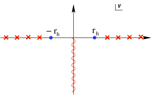
Figure 5.9: The analytic structure of the boundary Green’s function in the “ bubble of nothing” phase in the WKB approximation $\nu\to\infty$, $MR_{\rm AdS}\to\infty$ with $\tilde{\nu}=\nu/MR_{\rm AdS}$ fixed. Approximately equally spaced simple poles on the real axis for $\tilde{\nu}^{2}>\tilde{r}_{h}^{2}$, are accompanied by branch points at $\tilde{\nu}=0$ and infinity.

In terms of elliptic functions, the explicit form for the WKB action is

$$\begin{split}{\cal S}_{I}=&-\frac{MR_{\rm AdS}}{\sqrt{1+2\tilde{r}_{h}^{2}}}\;\left(|\tilde{\nu}|(F\left(\csc^{-1}\sqrt{a},\;\tfrac{a}{b}\right)-\sqrt{\tfrac{b}{a}}K\left(\tfrac{b}{a}\right))-\tfrac{1}{|\tilde{\nu}|}(1+\tilde{r}_{h}^{2})\;\sqrt{\tfrac{b}{a}}\Pi\left(a\big{|}\tfrac{b}{a}\right)\right)\\ &-\tfrac{1}{2}MR_{\rm AdS}\left(\ln\left(\tfrac{2\epsilon^{-2}}{|\tilde{\nu}|\,\sqrt{1+\tilde{r}_{h}^{2}}}\right)+i\,\pi\right),\end{split}$$ (5.99)

and the only singularity of this expression is the logarithmic singularity at $\tilde{\nu}=0$ which complements the singularity at $\tilde{\nu}=\infty$, found above.

5.2.3 Combining the Results

The resulting analytic structure of the Green’s function is summarized in Fig. (5.9), which is to be contrasted with corresponding Green’s function (at large mass and frequency) in the topological black hole phase in Fig. (5.5). As already dicussed earlier, the isolated poles on the real axis indicate glueball states and that the gauge theory is in the confined phase, wherein the radius of the spatial $S^{1}$ is much smaller than the $dS_{3}$ radius of curvature. This may be interpreted as a hadronized phase, where the de Sitter temperature being too low for the degrees of freedom to be deconfined.

In this context, we should point out that the high frequency WKB analysis, where the frequencies are much larger than the de Sitter cosmological constant, is basically a flat space limit and thus, the singularities of the Green’s functions may be interpreted in the standard way as in flat space. One feature of the propagator in the bubble of nothing phase whose origin is not entirely clear is the branch point singularity at $\tilde{\nu}=0$. A similar branch point at $\tilde{\nu}=-i$ was encountered in the high frequency limit in the topological black hole phase. The associated branch cut was a consequence of the apparent merger of the infinite set of quasinormal poles of the topological black hole, in the high frequency limit. We do not know of a similar interpretation of the branch cuts of (5.99) and Fig. (5.9).

[15pc] I am a being of Heaven and Earth, of thunder and lightning, of rain and wind, of the galaxies.Eden Ahbez (1908 - 1995)

6 Strongly Coupled Plasma in de Sitter Space

In the previous chapter, we saw that the AdS topological black hole geometry corresponds to the deconfined or plasma phase of the strongly coupled ${\cal N}=4$ supersymmetric Yang-Mills theory of $dS_{3}\times S^{1}$. In this chapter, we will study further the properties of the strongly coupled plasma.

6.1 R-current correlation functions

Real time response to perturbations of a conserved charge density can reveal interesting late time physics, such as hydrodynamic or diffusive relaxation. It is now well understood and established via holographic calculations in AdS black hole backgrounds that correlators of conserved global currents exhibit hydrodynamic and diffusion poles Policastro:2002se ; Son:2007vk . R-charge diffusion in the strongly coupled, high temperature ${\cal N}=4$ plasma was first discovered in Policastro:2002se and we have reviewed it in Section 3.3.2.2. The universal features of strongly coupled plasmas follow from the properties of the stretched horizon of AdS black holes Son:2007vk . It is therefore natural to ask whether the horizon in the topological AdS black hole geometry implies hydrodynamic behaviour of correlation functions in the dual field theory. The answer to this question will depend on the relevant time scales involved since the boundary field theory is formulated on an expanding background, namely $dS_{3}\times S^{1}$.

The strong coupling correlators for $SO(6)$ R-currents of ${\cal N}=4$ SUSY Yang-Mills theory on $dS_{3}\times S^{1}$ will be obtained holographically from the on-shell action for the $U(1)$ gauge fields in the topological $AdS_{5}$ black hole background, by following the prescription of Policastro:2002se . The Maxwell action for the gauge field is

$$S=-\frac{1}{4g^{2}_{\mathrm{SG}}}\int d^{5}x\sqrt{-g}g^{\mu\alpha}g^{\nu\beta}F_{\mu\nu}F_{\alpha\beta},$$ (6.1)

varying which gives the following equations of motion

$$\frac{1}{\sqrt{-g}}\partial_{\nu}\left(\sqrt{-g}g^{\mu\alpha}g^{\nu\beta}F_{\alpha\beta}\right)=0.$$ (6.2)

Here, we have $g_{\mathrm{SG}}^{2}=16\pi^{2}R_{\rm AdS}/N^{2}$. We find it convenient to use the following form for the metric in the region exterior to the horizon,

$$ds^{2}=\frac{R^{2}_{\rm AdS}}{4z^{2}\left(1-z\right)}dz^{2}+\frac{R^{2}_{\rm AdS}(1-z)}{z}\left[-d\tau^{2}+\cosh^{2}\tau\;d\Omega_{2}^{2}\right]+\frac{r_{\chi}^{2}}{z}\;d\chi^{2}.$$ (6.3)

Substituting the solution to the equation of motion that corresponds to the boundary value $A_{\alpha}(z)\big{|}_{z=0}=A_{\alpha}^{0}$ back into the gauge field action, we will get a generating functional for the R-charge correlators of the field theory.

Since the field theory lives on the $dS_{3}\times S^{1}$ boundary with spatial $S^{2}\times S^{1}$ spatial slices, it is natural to consider the late time behaviour of long-wavelength fluctuations in the following two cases:

1. The R-charge perturbation is inhomogeneous on the $S^{1}$, but homogeneous on the spatial section of $dS_{3}$,

2. The fluctuation is homogeneous on the circle, but inhomogeneous on the $S^{2}$.

Of particular interest is the presence or the lack of late time hydrodynamic relaxation of this system.

6.1.1 Inhomogeneous Perturbation on the $S^{1}$

In the first case, we will assume for simplicity that the R-charge perturbation carries no momentum around the $S^{2}$. Furthermore, we use gauge freedom to set the radial component of the gauge potential $A_{z}=0$. Hence, from the symmetries of the configuration, there are two remaining bulk gauge fields that are non zero:

$$A_{\tau}=A_{\tau}(z,\tau,\chi)\qquad{\rm and}\qquad A_{\chi}=A_{\chi}(z,\tau,\chi).$$ (6.4)

Since the $\chi$-direction is a spatial circle, the two components of the vector potential, $A_{\tau}$ and $A_{\chi}$, can be conveniently expanded in Fourier modes on the circle. The time dependence can also be re-expressed in terms of a mode expansion. There is a subtlety involved in this however. For $A_{\chi}$, which is a scalar in $dS_{3}$, the mode decomposition is straightforward

$$A_{\chi}(z,\tau,\chi)=\sum_{n}\frac{e^{in\chi}}{2\pi}\int_{-\infty}^{\infty}\frac{d\nu}{2\pi}\,\,{{\cal T}_{\chi}(\nu,\tau)}\;\;{\cal G}_{n}(\nu,z),$$ (6.5)

where $n\in\mathbb{Z}$. On the other hand, $A_{\tau}$, which is a gauge field in $dS_{3}$, has its complete time dependence captured by normal modes of two kinds: normalizable and delta-function normalizable. In fact, below we will show that there is a single normalizable mode and a continuum of delta-function normalizable states obtained as solutions to a Schrödinger problem. Anticipating this, we write

$$A_{\tau}(z,\tau,\chi)=\sum_{n}\frac{e^{in\chi}}{2\pi}\left(\int_{-\infty}^{\infty}\frac{d\nu}{2\pi}\,{\cal T}_{\tau}(\nu,\tau)\;{\cal F}_{n}(\nu,z)+{\cal T}_{\tau}^{\rm N}(\tau)\,{\cal F}^{{\rm N}}_{n}(z)\right),$$ (6.6)

where ${\cal T}_{\tau}(\nu,\tau)$ and ${\cal T}^{\rm N}_{\tau}(\tau)$ will be the delta-normalizable and normalizable modes, respectively. The mode functions ${\cal T}_{\chi,\tau}$ are solutions to

$$\frac{d}{d\tau}\left({\cosh^{-2}\tau}\,\frac{d}{d\tau}\left(\cosh^{2}\tau\,{\cal T}_{\tau}(\nu,\tau)\right)\right) =-(\nu^{2}+1)\;{\cal T}_{\tau}(\nu,\tau),$$ (6.7a)

$${\cosh^{-2}\tau}{d\over d\tau}\left(\cosh^{2}\tau\,{\cal T}_{\tau}\right) =-i(\nu+i){\cal T}_{\chi}.$$ (6.7b)

The first of these can be put in the form of a Schrödinger equation, by defining ${\cal T}_{\tau}=\tilde{\cal T}/\cosh\tau$,

$$-\frac{d^{2}}{d\tau^{2}}\tilde{\cal T}-{2\over\cosh^{2}\tau}\tilde{\cal T}=\nu^{2}\,\tilde{\cal T}.$$ (6.8)

It is solved by the associated Legendre function ${P}_{1}^{-i\nu}(\tanh\tau)$. For $\nu^{2}\geq 0$, there is a continuous infinity of delta-function normalizable states, which yield

$${\cal T}_{\tau}(\nu,\tau)=\,\frac{e^{-i\nu\tau}}{\cosh\tau}\left(\frac{\nu-i\tanh\tau}{\nu-i}\right)\qquad{\rm and}\qquad{\cal T}_{\chi}(\nu,\tau)=\frac{e^{-i\nu\tau}}{\cosh\tau},$$ (6.9)

where $\nu^{2}\geq 0.$

The Schrödinger potential above also has bound states for $\nu^{2}<0$. In fact, there is precisely one normalizable bound state with $\nu^{2}=-1$, corresponding to the solution

$${\cal T}_{\tau}^{\rm N}(\tau)={1\over\sqrt{2}}\,{1\over\cosh^{2}\tau}.$$ (6.10)

This solution can be directly obtained by evaluating $P_{1}^{-i\nu}(\tanh\tau)$ at $\nu^{2}=-1$ or can be systematically inferred from the Maxwell equations.

The continuum modes for $A_{\chi}$ and $A_{\tau}$ are orthonormal with respect to the inner product

$$\langle{\cal T}_{a},{\cal T}_{a}\rangle\equiv\int_{-\infty}^{\infty}d\tau\cosh^{2}\tau\;{\cal T}_{a}(\nu,\tau){\cal T}_{a}(\nu^{\prime},\tau)=2\pi\,\delta(\nu+\nu^{\prime}),$$ (6.11)

for $a\in\{\chi,\tau\}$, while the bound state is normalized so that

$$\int_{-\infty}^{\infty}d\tau\,\cosh^{2}\tau\,\left({\cal T}^{\rm N}_{\tau}\right)^{2}=1.$$ (6.12)

In the far future, the continuum modes are both given by ${\cal T}_{a}\sim e^{-i\nu\tau}e^{-2\tau}$. Upon analytically continuing to the complex $\nu$ plane, for $\nu=i+\omega$, with $\omega\in{\mathbb{R}}$, they are propagating, i.e., purely oscillatory, excitations with frequency $\omega$ in the far future. On the other hand the normalizable bound state decays exponentially in the far past and future. Furthermore, being real, it does not contribute to the flux at the horizon of the topological black hole.

Using these modes to eliminate the $\tau$-dependence, we find three equations that depend only on ${\cal F}_{n}(\nu,z)$ and ${\cal G}_{n}(\nu,z)$

$$-\tfrac{1}{R^{2}_{\rm AdS}}\,(\nu+i)\;{\cal F}_{n}^{\prime}+\frac{n(1-z)}{r_{\chi}^{2}}\,{\cal G}_{n}^{\prime} =0,$$ (6.13a)

$$\tfrac{1}{R^{2}_{\rm AdS}}\frac{d}{dz}\left((1-z){\cal F}_{n}^{\prime}\right)+\frac{n}{r_{\chi}^{2}}\,(\nu-i)\,{\cal G}_{n}-\frac{n^{2}}{r_{\chi}^{2}}\,{\cal F}_{n} =0,$$ (6.13b)

$$4z\frac{d}{dz}\left((1-z)^{2}{\cal G}_{n}^{\prime}\right)-n(\nu+i){\cal F}_{n}+(\nu^{2}+1){\cal G}_{n} =0.$$ (6.13c)

Here, prime denotes a derivative with respect to $z$. The radial or $z$-dependence of the bound state solution, ${\cal F}^{\rm N}(z)$ is found by analytically continuing the profile for generic $\nu$ to $\nu=\pm i$. We note that there are three equations for two unknowns. Therefore, to ensure a non-trivial solution, any two equations must imply the third and it is straightforward to check that this is indeed the case.

We can then use these equations of motion to derive two independent ones, each containing only one of the unknown functions:

$$4z(1-z){\cal F}_{n}^{\prime\prime\prime}-4(3z-1){\cal F}_{n}^{\prime\prime}-4{\cal F}_{n}^{\prime} =\left[\bar{n}^{2}-\frac{\nu^{2}+1}{1-z}\right]{\cal F}_{n}^{\prime},$$ (6.14a)

$$4z(1-z){\cal G}_{n}^{\prime\prime\prime}-4(5z-1){\cal G}_{n}^{\prime\prime}-\frac{8(1-2z)}{1-z}{\cal G}_{n}^{\prime} =\left[\bar{n}^{2}-\frac{(\nu^{2}+1)}{1-z}\right]{\cal G}_{n}^{\prime},$$ (6.14b)

where we have defined $\bar{n}\equiv\frac{nR_{\rm AdS}}{r_{\chi}}$.

Unfortunately, we cannot use the perturbative method as described in Section 3.3.2.2 in this case, as the smoothness condition used in the perturbative method is not enough to fully determine the solution. Fortunately, these equations of motion can be solved in terms of hypergeometric functions

$${\cal F}_{n}^{\prime}=C_{\tau}(\nu,\bar{n})\;(1-z)^{-i(\nu-i)/2}\;{}_{2}F_{1}\left(\tfrac{1}{2}+\tfrac{i}{2}(\bar{n}-\nu)\,,\tfrac{1}{2}-\tfrac{i}{2}(\bar{n}+\nu)\,;1-i\nu\,;1-z\right).$$ (6.15)

Here, $C_{\tau}$ is a frequency dependent constant, to be determined by the boundary values of the fields. Near the boundary of AdS space, the solution approaches

$$\begin{split}{\cal F}_{n}^{\prime}\big{|}_{z\to 0}=-\;C_{\tau}\;\tfrac{\Gamma(1-i\nu)}{\Gamma\left(\tfrac{1}{2}+\tfrac{i}{2}(\bar{n}-\nu)\right)\Gamma\left(\tfrac{1}{2}-\tfrac{i}{2}(\bar{n}+\nu)\right)}\,\left(2\gamma_{E}+\ln z+\psi\left(\tfrac{1}{2}+\tfrac{i}{2}(\bar{n}-\nu)\right)+\psi\left(\tfrac{1}{2}-\tfrac{i}{2}(\bar{n}+\nu)\right)\right).\end{split}$$ (6.16)

Imposing the boundary conditions at $z\to 0$

$$\lim_{\epsilon\to 0}{\cal F}_{n}(\nu,\epsilon)={\cal F}^{0}_{n}(\nu)\qquad{\rm and}\qquad\lim_{\epsilon\to 0}{\cal G}_{n}(\nu,\epsilon)={\cal G}_{n}^{0}(\nu),$$ (6.17)

from (6.13b), we find that

$$C_{\tau}(\nu,\bar{n})=-\tfrac{\Gamma\left(\tfrac{1}{2}+\tfrac{i}{2}(\bar{n}-\nu)\right)\Gamma\left(\tfrac{1}{2}-\tfrac{i}{2}(\bar{n}+\nu)\right)}{4\Gamma(1-i\nu)}\;\left(\bar{n}^{2}{\cal F}_{n}^{0}(\nu)-\tfrac{R_{\rm Ads}}{r_{\chi}}\,\bar{n}(\nu-i)\,{\cal G}^{0}_{n}(\nu)\right).$$ (6.18)

With the normalization fixed in terms of the boundary values of the relevant fields, we have

$$\begin{split}{\cal F}_{n}^{\prime}(\nu,\epsilon)=\tfrac{1}{4}\left(\bar{n}^{2}{\cal F}_{n}^{0}-\tfrac{R_{\rm AdS}}{r_{\chi}}\,\bar{n}(\nu-i){\cal G}_{n}^{0}\right)\;\left(2\gamma_{E}+\ln\epsilon+\psi\left(\tfrac{1}{2}+\tfrac{i}{2}(\bar{n}-\nu)\right)+\psi\left(\tfrac{1}{2}-\tfrac{i}{2}(\bar{n}+\nu)\right)\right).\end{split}$$ (6.19)

From (6.13a) we also obtain

$${\cal G}_{n}^{\prime}(\nu,\epsilon)=\tfrac{r_{\chi}}{R_{\rm AdS}}{\nu+i\over\bar{n}}{\cal F}_{n}^{\prime}(\nu,\epsilon).$$ (6.20)

Following identical steps for the normalizable temporal modes, we have

$${\cal F}_{n}^{{\rm N}\prime}(\epsilon)=\tfrac{1}{4}\bar{n}^{2}{\cal F}_{n}^{{\rm N}0}\left(2\gamma_{E}+\ln\epsilon+\psi\left(1+\tfrac{i}{2}\bar{n}\right)+\psi\left(1-\tfrac{i}{2}\bar{n}\right)\right).$$ (6.21)

We can now plug these solutions into the boundary action to obtain the retarded R-current correlators.

The induced boundary action for bulk Maxwell fields has the form

$$\begin{split}S={4\pi\over g^{2}_{SG}}\sum_{n}\frac{1}{2\pi}\,\left(\int_{-\infty}^{\infty}{d\nu\over 2\pi}\left(r_{\chi}{\cal F}_{-n}^{0}(-\nu)\;{\cal F}_{n}^{\prime}(\nu)\big{|}_{z=\epsilon}-\tfrac{R^{2}_{\rm AdS}}{r_{\chi}}\,{\cal G}_{-n}^{0}(-\nu)\;{\cal G}_{n}^{\prime}(\nu)\big{|}_{z=\epsilon}\right)+r_{\chi}{\cal F}_{-n}^{{\rm N}0}{\cal F}_{n}^{{\rm N}\prime}\big{|}_{z=\epsilon}\right),\end{split}$$ (6.22)

where $g^{2}_{SG}=16\pi^{2}R_{\rm AdS}/N^{2}$. The complete real time retarded correlation functions for the R-currents, can now be accessed readily. First, we define the boundary values of our gauge fields as

$$A_{\chi,\tau}(\epsilon,\tau,\chi)\equiv\sum_{n}{e^{in\chi}\over 2\pi}A_{\chi,\tau}^{n}(\tau)\,,$$ (6.23)

so that

$${\cal G}_{n}^{0}(-\nu)=\int_{-\infty}^{\infty}\,A_{\chi}^{n}(\tau)\,{\cal T}_{\chi}(\nu,\tau)\cosh^{2}\tau.$$ (6.24)

Similarly,

$${\cal F}^{0}_{n}(-\nu)=\int_{-\infty}^{\infty}\,A_{\tau}^{n}(\tau)\,{\cal T}_{\tau}(\nu,\tau)\cosh^{2}\tau\,\qquad{\rm and}\qquad{\cal F}^{{\rm N}0}_{n}=\int_{-\infty}^{\infty}\,A_{\tau}^{n}(\tau)\,{\cal T}_{\tau}^{\rm N}(\tau)\cosh^{2}\tau\,.$$ (6.25)

Putting these ingredients together, we find that the boundary action is

$$\begin{split}S=&{N^{2}\over 4\pi R_{\rm AdS}}\;\sum_{n}\tfrac{1}{2\pi}\int_{-\infty}^{\infty}d\tau\,\cosh^{2}\tau\int_{-\infty}^{\infty}d\tau^{\prime}\,\cosh^{2}\tau^{\prime}\\ &\left[\int_{-\infty}^{\infty}{d\nu\over 2\pi}\left(2\gamma_{E}+\ln\epsilon+\psi\left(\tfrac{1}{2}+\tfrac{i}{2}(\bar{n}-\nu)\right)+\psi\left(\tfrac{1}{2}-\tfrac{i}{2}(\bar{n}+\nu)\right)\right)\times\right.\\ &\left.\times\left(\,A_{\tau}^{-n}(\tau)A_{\tau}^{n}(\tau^{\prime})\,\tfrac{{\bar{n}}^{2}}{4}\,r_{\chi}\,\,{\cal T}_{\tau}(\nu,\tau){\cal T}_{\tau}(-\nu,\tau^{\prime})\,-\,A_{\tau}^{-n}(\tau)A_{\chi}^{n}(\tau^{\prime})\,{R_{\rm AdS}}\tfrac{\bar{n}}{4}(\nu-i)\,\times\right.\right.\\ \\ &\left.\left.\times{\cal T}_{\tau}(\nu,\tau){\cal T}_{\chi}(-\nu,\tau^{\prime})\,-\,A_{\chi}^{-n}(\tau)A_{\tau}^{n}(\tau^{\prime})\,R_{\rm AdS}\tfrac{\bar{n}}{4}(\nu+i)\,{\cal T}_{\chi}(\nu,\tau){\cal T}_{\tau}(-\nu,\tau^{\prime})\,+\right.\right.\\ \\ &\left.\left.+A_{\chi}^{-n}(\tau)A_{\chi}^{n}(\tau^{\prime})\tfrac{R^{2}_{\rm AdS}}{r_{\chi}}\tfrac{1}{4}(\nu^{2}+1){\cal T}_{\chi}(\nu,\tau){\cal T}_{\chi}(-\nu,\tau^{\prime})\right)+r_{\chi}A^{-n}_{\tau}(\tau)A^{n}_{\tau}(\tau^{\prime})\times\right.\\ \\ &\left.\times\tfrac{{\bar{n}}^{2}}{4}{\cal T}^{\rm N}(\tau){\cal T}^{\rm N}(\tau^{\prime})\left(2\gamma_{E}+\ln\epsilon+\psi\left(1+\tfrac{i}{2}\bar{n}\right)+\psi\left(1-\tfrac{i}{2}\bar{n}\right)\right)\right].\end{split}$$ (6.26)

The R-current correlators can be read off from the finite and non-analytic pieces of this boundary action (6.22), (6.26). We will denote the Fourier harmonics of the R-current along the spatial circle as

$$j_{n}^{\mu}(\tau)=\int_{0}^{2\pi}d\chi\,e^{-in\chi}\,j^{\mu}(\chi,\tau),$$ (6.27)

where we have already restricted attention to the s-wave sector on the spatial two-sphere. For perturbations with non-vanishing momentum along the spatial circle, we define the retarded, real time, Green’s functions as

$$G^{\mu\nu}(\tau,\tau^{\prime};n)=\langle[\,j_{n}^{\mu}(\tau),\,j_{-n}^{\nu}(\tau^{\prime})]\rangle\,\Theta(\tau-\tau^{\prime})\,,\qquad\mu,\nu\in\{\chi,\tau\}.$$ (6.28)

The conserved global currents are in one-to-one correspondence with the boundary values of the 5-d gauge fields. Functionally differentiating the induced boundary action (6.26) with respect to the boundary values of the gauge fields, we find

$$G^{\tau\tau}(\tau,\tau^{\prime};n)= \,\cosh^{2}\tau\cosh^{2}\tau^{\prime}\,\times$$ (6.29a)

$$\qquad n^{2}\,\left[\int_{-\infty}^{\infty}{d\nu\over 2\pi}\,{\cal T}_{\tau}(\nu,\tau){\cal T}_{\tau}(-\nu,\tau^{\prime})\,\,{\bf\Xi}(\nu,n)+{\cal T}_{\tau}^{\rm N}(\tau){\cal T}_{\tau}^{\rm N}(\tau^{\prime})\,\,{\bf\Xi}(i,n)\right],$$

$$G^{\chi\chi}(\tau,\tau^{\prime};n)= \,\cosh^{2}\tau\cosh^{2}\tau^{\prime}\int_{-\infty}^{\infty}{d\nu\over 2\pi}\,{\cal T}_{\chi}(\nu,\tau){\cal T}_{\chi}(-\nu,\tau^{\prime})\left(\nu^{2}+1\right)\,{\bf\Xi}(\nu,\,n),$$ (6.29b)

$$G^{\tau\chi}(\tau,\tau^{\prime};n)= \,G^{\chi\tau\,*}(\tau,\tau^{\prime};n)=\,\cosh^{2}\tau\cosh^{2}\tau^{\prime}\,n\int_{-\infty}^{\infty}{d\nu\over 2\pi}\,{\cal T}_{\tau}(\nu,\tau){\cal T}_{\chi}(-\nu,\tau^{\prime})\left(\nu-i\right){\bf\Xi}(\nu,n),$$ (6.29c)

where

$${\bf\Xi}(\nu,\,n)=\tfrac{N^{2}R_{\rm AdS}}{32\pi^{2}r_{\chi}}\left(\psi\left(\tfrac{1}{2}+\tfrac{i}{2}(\bar{n}-\nu)\right)+\psi\left(\tfrac{1}{2}-\tfrac{i}{2}(\bar{n}+\nu)\right)\right).$$ (6.30)

It is easily established that the above expressions are indeed retarded Green’s functions and are non-vanishing only when $\tau>\tau^{\prime}$. Two essential features ensure that this is the case:

1. The function ${\bf\Xi}(\nu,n)$ appearing universally in the $\nu$-integrals has only simple poles in the lower half complex plane at

   $$\nu=-i(2k+1)\pm\bar{n}\,,\qquad k\in{\mathbb{Z}}.$$ (6.31)

2. There is a second source of non-analyticities in the $\nu$-plane. This lies in the $\nu$-dependent normalization of the mode functions ${\cal T}_{\tau}(\nu,\tau)$ (6.9). The potentially worrisome aspect of this is the appearance of a pole in the upper half plane at $\nu=+i$, which gives a non-vanishing contribution for $\tau<\tau^{\prime}$. However, the potential problem is eliminated by the term dependent on the discrete, normalizable mode ${\cal T}^{N}_{\tau}$ in (6.29) which exactly cancels against the contributions from the poles at $\nu=+i$, ensuring that our Green’s function is causal.

The remaining Green’s functions are manifestly free of singularities in the upper half plane. We thus see that the Son-Starinets recipe for determining real time response functions works in the case of the topological black hole, provided we carefully account for the contributions from both the continuum and discrete mode functions in $dS_{3}$.

It is also clear in the above expressions that there are no diffusion poles. Instead, from the properties of the digamma function which we have encountered before, the frequency space Green’s function, which is effectively ${\bf\Xi}(\nu,n)$ , has only simple poles in the complex $\nu$-plane, the lowest of these being at

$$\nu=-i\pm\,\bar{n}.$$ (6.32)

Excitations with complex $\nu=\omega-i$, and $\omega\in{\mathbb{R}}$ will propagate at late times, where the perturbations simply evolve as left- and right-moving excitations on the $S^{1}$ without dissipating.

The absence of any diffusion or transport like behaviour may be intuitively explained by noticing the similarity of the topological AdS black hole to the BTZ black hole. Setting up an excitation with momentum only on the $S^{1}$ is equivalent to stating that the variation of the fields along the $S^{2}$ is zero. Therefore, aside from the time dependent factors associated to the de Sitter expansion, the metric that is “seen” by the bulk fields is not the full five dimensional metric, but its effective $2+1$ dimensional portion

$$ds^{2}=-R^{2}_{\rm AdS}(\rho^{2}-1)d\tau^{2}+\frac{R^{2}_{\rm AdS}}{\rho^{2}-1}d\rho^{2}+\rho^{2}r_{\chi}^{2}d\chi^{2}.$$ (6.33)

Comparing this with the metric for a $2+1$ dimensional BTZ black hole with zero angular momentum

$$ds^{2}=-\left(\frac{r^{2}}{R^{2}}-M\right)dt^{2}+\left(\frac{r^{2}}{R^{2}}-M\right)^{-1}dr^{2}+r^{2}d\phi^{2},$$ (6.34)

we note the obvious similarity. Therefore, we expect the behaviour of fields in the topological black hole background with an inhomogeneous excitation around the $S^{1}$ to be similar to the behaviour of the fields in a BTZ black hole background. In other words, they should behave as in a (1+1)-dimensional CFT Son:2002sd , just as we see from our results above.

6.1.2 Inhomogeneous Perturbation on the $S^{2}$

We will now examine the real time response to fluctuations carrying momentum along the spatial sections of the three dimensional de Sitter space. Each spatial section of $dS_{3}$ is a two-sphere which undergoes exponential expansion at late times. For this case, we will focus on a situation where an inhomogeneous R-charge perturbation is set up on the two-sphere with only a dependence on the polar angle $\theta$ and time $\tau$. For this configuration, the dual bulk gauge fields are

$$A_{\tau}=A_{\tau}(z,\tau,\theta)\,\qquad{\rm and}\qquad A_{\theta}=A_{\theta}(z,\tau,\theta)\,,$$ (6.35)

where $A_{z}=A_{\chi}=0$. Here, $A_{z}$ is set to zero by the gauge freedom and $A_{\chi}$ vanishes due to $\chi$-independence of the configuration.

By spherical symmetry, the scalar potential $A_{\tau}$ and the vector potential $A_{\theta}$, each can be expanded in terms of scalar and vector spherical harmonics, respectively:

$$A_{\tau}=\sum_{\ell=0}^{\infty}{\cal F}_{\ell}(z,\tau)\;Y_{\ell}^{0}(\theta),\qquad A_{\theta}=\sum_{\ell=1}^{\infty}{\cal G}_{\ell}(z,\tau)\;\partial_{\theta}Y_{\ell}^{0}(\theta).$$ (6.36)

Substituting these into the bulk Maxwell equations, we find

$$4z(1-z){\partial_{z}}\left((1-z){\partial_{z}{\cal G}_{\ell}}\right)-{\partial^{2}_{\tau}{\cal G}_{\ell}}+{\partial_{\tau}{\cal F}_{\ell}}= \,0,$$ (6.37a)

$$4z(1-z)\partial_{z}\left((1-z){\partial_{z}{\cal F}_{\ell}}\right)-{\ell(\ell+1)\over\cosh^{2}\tau}\left({\cal F}_{\ell}-\partial_{\tau}{\cal G}_{\ell}\right)= \,0,$$ (6.37b)

$$\partial_{\tau}\left(\cosh^{2}\tau\partial_{z}{\cal F}_{\ell}\right)+\ell(\ell+1)\partial_{z}{\cal G}_{\ell}= \,0.$$ (6.37c)

From equations (6.37b) and (6.37c) we obtain a differential equation for ${\cal F}^{\prime}_{\ell}\equiv\partial_{z}{\cal F}_{\ell}$

$$4\partial_{z}\left(z(1-z)\partial_{z}\left((1-z){\cal F}^{\prime}_{\ell}\right)\right)-{\ell(\ell+1)\over\cosh^{2}\tau}{\cal F}^{\prime}_{\ell}-{1\over\cosh^{2}\tau}\partial_{\tau}^{2}\left(\cosh^{2}\tau{\cal F}^{\prime}_{\ell}\right)=0.$$ (6.38)

Now, we will separate out the explicit temporal dependence, keeping in mind, as before, the possibility of contributions from both discrete and continuous modes

$${\cal F}^{\prime}_{\ell}(z,\tau)=\int_{-\infty}^{\infty}{d\nu}\;{\cal T}_{\ell}(\nu,\tau)\;F_{\ell}(\nu,z)+\sum_{m}{\cal T}_{\ell\,m}^{\rm N}(\tau)\,F_{\ell\,m}^{\rm N}(z).$$ (6.39)

The mode functions ${\cal T}_{\ell}$ satisfy

$$\left[-\partial_{\tau}^{2}-{\ell(\ell+1)\over\cosh^{2}\tau}\right]\left(\cosh^{2}\tau\,{\cal T}_{\ell}\right)=\nu^{2}\;\left(\cosh^{2}\tau\,{\cal T}_{\ell}\right),$$ (6.40)

which is a Schrödinger equation whose potential clearly will have both bound states and scattering or continuum states. The full set of solutions form an orthonormal, complete set. Indeed, the delta-normalized eigenstates are the Legendre functions

$${\cal T}_{\ell}(\nu,\tau)=\Gamma(1+i\nu)\,{P_{\ell}^{-i\nu}(\tanh\tau)\over\cosh^{2}\tau}.$$ (6.41)

Those with $\nu^{2}>0$ are scattering states with continuous values of $\nu\in{\mathbb{R}}$, while the discrete, “bound states” have $-i\nu=1,2,\ldots\ell$,

$${\cal T}_{\ell\,m}^{\rm N}=\sqrt{m(\ell-m)!\over(\ell+m)!}\,\,{P_{\ell}^{m}(\tanh\tau)\over\cosh^{2}\tau}\,,\qquad m=1,2,\ldots\ell.$$ (6.42)

For $\nu^{2}>0$, the late time $\tau\to\infty$ behaviour of the modes will be significant,

$${\cal T}_{\ell}(\nu,\tau)\big{|}_{\tau\gg 1}\to e^{-i\nu\tau}\;e^{-2\tau},$$ (6.43)

as these modes are oscillatory. Applying infalling boundary conditions on these modes at the horizon of the topological AdS black hole, (6.38) yields

$$F_{\ell}(\nu,z)=C_{\ell}(\nu)\;(1-z)^{-1-i\nu/2}\;{}_{2}F_{1}\;\left(-i\tfrac{\nu}{2},1-i\tfrac{\nu}{2}\,;1-i\nu\,;1-z\right).$$ (6.44)

For the discrete series, the radial profile in the bulk $F_{\ell\,m}^{\rm N}(z)$ is obtained by evaluating $F_{\ell}(\nu,z)$ at $\nu=-im$.

The asymptotic form of the radial dependence of the bulk potential ${\cal F}^{\prime}_{\ell}$, can be determined from (6.44)

$$F_{\ell}\big{|}_{z\to 0}=C_{\ell}(\nu)\left(C_{1}(\nu)+C_{2}(\nu)\;\ln z\right),$$ (6.45)

where

$$C_{1}=-\frac{2\gamma_{E}+\psi(1-\tfrac{i\nu}{2})+\psi(-\tfrac{i\nu}{2})}{\Gamma(1-\tfrac{i\nu}{2})\Gamma(-\tfrac{i\nu}{2})},$$ (6.46a)

$$C_{2}=-{1\over\Gamma(1-\tfrac{i\nu}{2})\Gamma(-\tfrac{i\nu}{2})}.$$ (6.46b)

We can solve for $C_{\ell}$ in terms of the boundary values of the gauge potentials, using the bulk equation of motion (6.37b) for ${\cal F}_{\ell}^{\prime}$ near the boundary which yields

$$4\int_{-\infty}^{\infty}{d\nu\over 2\pi}\;\Gamma(1+i\nu)P_{\ell}^{-i\nu}(\tanh\tau)\;\ C_{\ell}(\nu)\;C_{2}(\nu)=\ell(\ell+1)\left({\cal F}_{\ell}^{0}(\tau)-\partial_{\tau}{\cal G}_{\ell}^{0}(\tau)\right).$$ (6.47)

We note that the other equation of motion (6.37a) for ${\cal G}_{\ell}^{\prime}$, just yields the time derivative of this condition, so that we have only one equation to determine the coefficient $C_{\ell}$. This equation can be solved if we recall that the associated Legendre functions are mutually orthogonal

$$\int_{-\infty}^{\infty}d\tau\;P_{\ell}^{i\nu}(\tanh\tau)P_{\ell}^{-i\nu^{\prime}}(\tanh\tau)={\delta(\nu-\nu^{\prime})\over\Gamma(1-i\nu)\Gamma(1+i\nu)}.$$ (6.48)

Thus, we have

$$C_{\ell}={\ell(\ell+1)\over 4C_{2}}\Gamma(1-i\nu)\int_{-\infty}^{\infty}d\tau^{\prime}\left({\cal F}_{\ell}^{0}(\tau^{\prime})-\partial_{\tau^{\prime}}{\cal G}_{\ell}^{0}(\tau^{\prime})\right)\;P_{\ell}^{i\nu}(\tanh\tau^{\prime}),$$ (6.49)

from which we obtain the solution

$$\begin{split}\cosh^{2}\tau\;{\cal F}^{\prime}_{\ell}(\epsilon,\tau)=&\;{\ell(\ell+1)\over 4}\,\int_{-\infty}^{\infty}d\tau^{\prime}\left({\cal F}_{\ell}^{0}(\tau^{\prime})-\partial_{\tau^{\prime}}{\cal G}_{\ell}^{0}(\tau^{\prime})\right)\\ &\bigg{[}\int_{-\infty}^{\infty}{d\nu\over 2\pi}\,{\pi\nu\over\sinh\pi\nu}\;P_{\ell}^{-i\nu}(\tanh\tau)P_{\ell}^{i\nu}(\tanh\tau^{\prime})\,\left(\ln\epsilon+2\gamma_{E}+\psi(-\tfrac{i\nu}{2})+\psi(1-\tfrac{i\nu}{2})\right)\\ &+\sum_{m=1}^{\ell}m\tfrac{(\ell-m)!}{(\ell+m)!}\,P_{\ell}^{m}(\tanh\tau)P_{\ell}^{m}(\tanh\tau^{\prime})\left(\ln\epsilon+2\gamma_{E}+\psi\left(\tfrac{m}{2}\right)+\psi(1+\tfrac{m}{2})\right)\bigg{]}.\end{split}$$ (6.50)

Plugging these back into the expression for the boundary action (6.53), we obtain the generating functional for two point correlators of R-currents.

Putting the above ingredients together, the general form of the electric field along the radial direction in the bulk is

$$A_{\tau}^{\prime}(z,\tau,\theta)=\sum_{\ell=0}^{\infty}Y_{\ell}^{0}(\theta)\left(\int_{-\infty}^{\infty}\;{d\nu\over 2\pi}\,{\Gamma(1+i\nu)}\,{P_{\ell}^{-i\nu}(\tanh\tau)\over\cosh^{2}\tau}\;F_{\ell}(\nu,z)+\sum_{m=1}^{\ell}\sqrt{m\tfrac{(\ell-m)!}{(\ell+m)!}}\,{P_{\ell}^{m}(\tanh\tau)\over\cosh^{2}\tau}\,F_{\ell\,m}^{\rm N}(z)\right).$$ (6.51)

This also allows us to automatically solve for $A_{\theta}^{\prime}$ using (6.37c) and we get

$$A_{\theta}^{\prime}(z,\tau,\theta)=-\sum_{\ell=1}^{\infty}{\partial_{\theta}Y_{\ell}^{0}(\theta)\over\ell(\ell+1)}\,\left(\int_{-\infty}^{\infty}{d\nu\over 2\pi}\;\Gamma(1+i\nu)\,\partial_{\tau}P_{\ell}^{-i\nu}(\tanh\tau)\;F_{\ell}(\nu,z)+\sum_{m=1}^{\ell}\sqrt{m\tfrac{(\ell-m)!}{(\ell+m)!}}\,\,\partial_{\tau}P_{\ell}^{m}(\tanh\tau)\,F_{\ell\,m}^{\rm N}(z)\right).$$ (6.52)

Now, the bulk gauge field action can be shown to induce a boundary term which will be the generating functional for the boundary R-current correlators. Using the explicit solutions above, the induced boundary action becomes

$$S={1\over 2g^{2}_{SG}}\int d\tau\;r_{\chi}\left[\sum_{\ell=0}^{\infty}{\cal F}_{\ell}(z,\tau)\,{\cal F}^{\prime}_{\ell}(z,\tau)\cosh^{2}\tau+\sum_{\ell=1}^{\infty}\ell(\ell+1)\,{\cal G}_{\ell}(z,\tau)\,{\cal G}^{\prime}_{\ell}(z,\tau)\right]_{z=\epsilon\to 0}.$$ (6.53)

The next step is to express this completely in terms of the boundary values of the gauge potentials ${\cal F}_{\ell}^{0}(\tau)\equiv{\cal F}_{\ell}(\epsilon,\tau)$ and ${\cal G}_{\ell}^{0}(\tau)\equiv{\cal G}_{\ell}(\epsilon,\tau)$. Their radial derivatives ${\cal F_{\ell}}^{\prime}$ and ${\cal G}_{\ell}^{\prime}$, equivalently $A_{\tau}^{\prime}$ and $A_{\theta}^{\prime}$, at the boundary $z=\epsilon$, are also determined completely by the boundary values of the gauge potentials, ${\cal F}_{\ell}^{0}(\tau)$ and ${\cal G}_{\ell}^{0}(\tau)$ as in (6.50).

From the boundary action above, we thus find that the real time, retarded Green’s functions for the R-charge currents $j^{\mu}$, in the gauge theory are

$$G^{\tau\tau}(\tau,\tau^{\prime};\ell)= \,\ell(\ell+1)\left[\int_{-\infty}^{\infty}{d\nu\over 2\pi}\;\,{\pi\nu\over\sinh\pi\nu}\;P_{\ell}^{-i\nu}(\tanh\tau)P_{\ell}^{i\nu}(\tanh\tau^{\prime})\,{\bf\Upsilon}(\nu)+\right.$$ (6.54a)

$$\left.\qquad\quad+\sum_{m=1}^{\ell}\,(-1)^{m}\,m\,P_{\ell}^{m}(\tanh\tau)P_{\ell}^{-m}(\tanh\tau^{\prime})\,{\bf\Upsilon}(i\,m)\right],$$

$$G^{\theta\theta}(\tau,\tau^{\prime};\ell)= \,\ell(\ell+1)\left[\int_{-\infty}^{\infty}{d\nu\over 2\pi}\;{\pi\nu\over\sinh\pi\nu}\;\partial_{\tau}P_{\ell}^{-i\nu}(\tanh\tau)\,\partial_{\tau^{\prime}}P_{\ell}^{i\nu}(\tanh\tau^{\prime}){\bf\Upsilon}(\nu)+\right.$$ (6.54b)

$$\left.\qquad\quad+\sum_{m=1}^{\ell}\,(-1)^{m}\,m\,\partial_{\tau}P_{\ell}^{m}(\tanh\tau)\partial_{\tau^{\prime}}P_{\ell}^{-m}(\tanh\tau^{\prime})\,{\bf\Upsilon}(i\,m)\right],$$

$$G^{\tau\theta}(\tau,\tau^{\prime};\ell)= \ell(\ell+1)\left[\int_{-\infty}^{\infty}{d\nu\over 2\pi}\;{\pi\nu\over\sinh\pi\nu}\;P_{\ell}^{-i\nu}(\tanh\tau)\,\partial_{\tau^{\prime}}P_{\ell}^{i\nu}(\tanh\tau^{\prime})\,{\bf\Upsilon}(\nu)+\right.$$ (6.54c)

$$\left.\qquad\quad+\sum_{m=1}^{\ell}(-1)^{m}\,m\,P_{\ell}^{m}(\tanh\tau)\partial_{\tau^{\prime}}P_{\ell}^{-m}(\tanh\tau^{\prime})\,{\bf\Upsilon}(i\,m)\right],$$

where

$${\bf\Upsilon}(\nu)=\tfrac{N^{2}r_{\chi}}{64\pi^{2}R_{\rm AdS}}\,\left(\psi(-\tfrac{i\nu}{2})-\tfrac{1}{i\nu})\right).$$ (6.55)

We need to first confirm that these Green functions satisfy basic consistency checks. Specifically, the retarded functions must vanish for $\tau<\tau^{\prime}$. As in the previous case, this property is not manifest, but follows from the nature of the non-analyticities of ${\bf\Upsilon}(\nu)$, and the normalized mode functions $\Gamma(1+i\nu)P_{\ell}^{-i\nu}(\tanh\tau)$, in the complex $\nu$-plane. For real values of $\nu$, the associated Legendre function is elliptic ; Abramowitz:1964

$$\Gamma(1+i\nu)\,P_{\ell}^{-i\nu}(\tanh\tau)=e^{-i\nu\tau}\,{}_{2}F_{1}(-\ell,\,\ell+1;\,1+i\nu,\,(1-\tanh\tau)/2).$$ (6.56)

For integer $\ell$, the hypergeometric function is a finite polynomial in $\tanh\tau$ and a ratio of degree $\ell$ polynomials of $\nu$. Therefore, the exponential frequency dependence means that, for $\tau-\tau^{\prime}<0$, the integrals over the frequency $\nu$ can be evaluated by closing the contour in the upper half plane. The function ${\bf\Upsilon}(\nu)$ has no poles in the upper half complex plane. It has simple poles at

$$\nu=0,\,-2i,\,-4i\ldots$$ (6.57)

The normalized modes, $\Gamma(1+i\nu)P_{\ell}^{-i\nu}(\tanh\tau)$ have exactly $\ell$ simple poles in the upper half plane at $\nu=i,\,2i\ldots\ell i$. The contributions from these are, however, cancelled by the inclusion of the discrete modes in the retarded Green’s function above. Hence, our correlators are zero for $\tau<\tau^{\prime}$.

6.1.3 Late Time Behavior

The real time response functions in general contain important information on the long time relaxation of perturbations away from the equilibrium or ground state. In thermal field theory on flat space, the relaxation of such fluctuations of conserved charges proceeds via hydrodynamic or diffusion modes. The response functions at strong coupling then exhibit diffusion poles in frequency space, $G^{\tau\tau}\propto(i\omega-Dk^{2})^{-1}$, where $\omega$ is the frequency and $k$, the soft spatial momentum. Due to the explicit time dependence of the background metric, we cannot do a similar frequency space study of the full Green’s functions in de Sitter space. Instead, we could analyze their behaviour as functions of time.

In de Sitter space, perturbations labelled by wave number $\ell$, get red-shifted so that given sufficient time, their physical wavelengths become super-horizon sized. This happens when

$${\ell\,e^{-\tau}\over R}\sim{1\over R}.$$ (6.58)

At late enough times, even very high harmonics on the sphere get stretched and eventually exit the horizon. To zoom in on the time evolution of such modes, it is useful to think of $\ell e^{-\tau}$, the physical wave number, as being fixed as $\tau\to\infty$. For example, in this late time approximation, we neglect terms like $\ell\,e^{-2\tau}$ in comparison to powers of $\ell\,e^{-\tau}$. This is practically equivalent to going to planar coordinates for de Sitter space and the mode functions behave as

$$P_{\ell}^{-i\nu}(\tanh\tau)\big{|}_{\ell e^{-\tau}=\,{\rm fixed}}\longrightarrow\ell^{-i\nu}\,J_{i\nu}\left(2\ell e^{-\tau}\right).$$ (6.59)

It is possible to derive this by replacing the potential $\ell(\ell+1){\rm sech}^{2}\tau$ in the mode equation (6.40), with $4\,\ell^{2}\,e^{-2\tau}$. We note that, instead of a fixed physical wavelength, if we focus attention on fixed comoving wavenumber, which is given by $\ell$, all modes simply approach the $s$-wave at late times

$$\lim_{\tau\to\infty}\,\Gamma(1+i\nu)\,P_{\ell}^{-i\nu}(\tanh\tau)\big{|}_{\ell\,\,{\rm fixed}}\longrightarrow e^{-i\nu\tau}.$$ (6.60)

For fixed physical wavelengths, $\ell\,e^{-\tau}$, or equivalently, at the time when a harmonic $\ell$ crosses the horizon, the real time correlators are given by the exact results with the replacement (6.59). The integral over $\nu$ can be easily evaluated using the method of residues, and it turns out that the leading contribution at late times is from the residue at $\nu=0$. Thus,

$$G^{\tau\tau}(\tau,\,0;\ell),\,\,\,G^{\tau\theta}(\tau,\,0;\ell)\,\,\sim\,\,J_{0}(2\,\ell e^{-\tau})$$ (6.61)

and

$$G^{\theta\tau}(\tau,0;\,\ell),\,\,\,G^{\theta\theta}(\tau,0;\,\ell)\,\,\sim\,\,\partial_{\tau}J_{0}(2\,\ell e^{-\tau}).$$ (6.62)

This late time behaviour is depicted in Figs. (6.1) and (6.2).

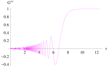
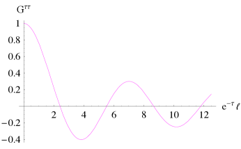
Fig. 6.1: The leading behaviour of correlators $G_{\tau\tau}$ (and $G_{\tau\theta}$), up to normalization constants: as a function of $\tau$ on the left with $\ell=1000$ and, on the right, as a function of $\ell e^{-\tau}$

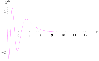
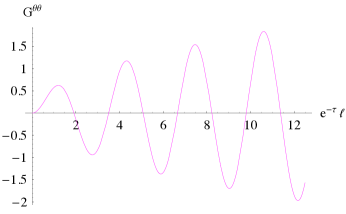
Fig. 6.2: The leading behaviour of $G_{\theta\theta}$ (and $G_{\theta\tau}$): The left figure is plotted as a function of time for $\ell=1000$, while the right hand side figure is a function of $\ell e^{-\tau}$.

The late time behaviour deduced above is not characteristic of diffusion in de Sitter space. Suppose that the R-charge fluctuation relaxed via diffusion modes, then the covariant conservation of the R-current together with Fick’s law would lead to the diffusion equation

$$\partial_{\tau}j^{\tau}=D\nabla_{\theta}\nabla^{\theta}\,j^{\tau},$$ (6.63)

in $dS_{3}$, $D$ being the diffusion constant. The spherical harmonics of $j^{\tau}$ on the expanding spatial spherical sections would then obey

$$\partial_{\tau}j^{\tau}_{\ell}=-D\,{\ell(\ell+1)\over\cosh^{2}\tau}\,j^{\tau}_{\ell}.$$ (6.64)

At late times $\tau\to\infty$ and large enough $\ell$, this is solved by

$$j^{\tau}_{\ell}\sim\exp\left(\tfrac{1}{2}D\,\ell^{2}\,e^{-2\tau}\right).$$ (6.65)

The large time behaviour of the Green’s functions (6.61) and (6.62) do not match up with expected diffusive relaxation (6.65) on $dS_{3}$. A natural reason for this is that the rate of exponential expansion of the spatial section and the Gibbons-Hawking temperature are both set by $R_{\rm dS}^{-1}$. Thus, the mean free path or the mean free time between collisions is comparable to the expansion time scales so that the system never enters a diffusive regime.

[15pc] Give me ambiguity or give me something else. Anonymous

7 Vacuum Ambiguity in de Sitter Space at Strong Coupling

In previous chapters, we saw that the Son-Starinets prescription automatically chose the boundary field theory to be in the Euclidean or Bunch-Davies vacuum. In this chapter, we will calculate the symmetric two-point functions at strong coupling and address the issue of vacuum ambiguity in de Sitter space at strong coupling.

This chapter is organized as follows. In Section 7.1, we review the issue of vacuum ambiguity in de Sitter space at the weak coupling regime. In Section 7.2, we perform the holographic computation of the symmetric two-point functions as functions of the geodesic distance.

7.1 $\alpha$-vacua in de Sitter Space

As we reviewed in Section 4.1, the three-dimensional de Sitter space $dS_{3}$ can be realized as the hypersurface described by

$$-x_{0}^{2}+x_{1}^{2}+x_{2}^{2}+x_{3}^{2}=R_{\rm dS}^{2},$$ (7.1)

with $R_{\rm dS}$ being the $dS_{3}$ radius. The metric for the global patch is given by

$$ds^{2}=-dt^{2}+R_{\rm dS}^{2}\cosh^{2}\left({t\over R_{\rm dS}}\right)\;d\Omega_{2}^{2}.$$ (7.2)

For a more detailed discussions on the classical geometry of de Sitter space and its other aspects see for example Spradlin:2001pw .

This spacetime does not contain a globally time-like Killing vector and thus does not have a unique vacuum state. To see this in a more formal manner, let us consider the symmetric two-point function in a de Sitter invariant state $|\alpha\rangle$. For simplicity, we consider only a free massive scalar field theory here. For the treatment of weakly interacting theories, see Collins:2003mj and references therein.

$|\alpha\rangle$ being de Sitter invariant implies that the symmetric two-point function $G_{\alpha}(x,y)$ can only depend on the two spacetime points $x$ and $y$ via the geodesic distance $d(x,y)$. The symmetric two-point function obeys the massive scalar field equation

$$\left(-\Box_{x}+m^{2}\right)G(x,y)=0,$$ (7.3)

which can be expressed as

$$\left(Z^{2}-1\right)^{-1/2}\partial_{Z}\left[\left(Z^{2}-1\right)^{3/2}\,\partial_{Z}G\left(Z(x,y)\right)\right]+m^{2}\,R_{\rm dS}^{2}\,G\left(Z(x,y)\right)=0,$$ (7.4)

where we have introduced the real function

$$Z(x,y)=\cos{d(x,y)\over R_{\rm dS}}\,.$$ (7.5)

Here, the mass term may include the contribution that comes from coupling to the curvature.

A solution is given by

$$G_{E}\left(Z(x,y)\right)={\Gamma(h_{+})\,\Gamma(h_{-})\over(4\pi)^{3/2}\,\Gamma(3/2)}\,\,_{2}F_{1}\left(h_{+},h_{-};{3\over 2};{1+Z(x,y)\over 2}\right),$$ (7.6)

with

$$h_{\pm}=1\pm\sqrt{1-m^{2}R_{\rm dS}^{2}}\,\,.$$ (7.7)

Here, the normalization is chosen such that the short distance singularity matches to that of Minkowski space.

We note that if $G_{E}(Z)$ is a solution to Eq. (7.4), then $G_{E}(-Z)$ is also a solution. Since for $m^{2}>0$ these two solutions are linearly independent, then the general solution to Eq. (7.4) can be expressed as

$$G_{\alpha}(x,y)={1+e^{\alpha+\alpha^{*}}\over 1-e^{\alpha+\alpha^{*}}}\,G_{E}\left(Z(x,y)\right)+{e^{\alpha}+e^{\alpha^{*}}\over 1-e^{\alpha+\alpha^{*}}}\,G_{E}\left(-Z(x,y)\right).$$ (7.8)

The constants in the $\alpha$-vacuum propagator (7.8) are chosen such that the modes of the free massive scalar field $\Phi$ in the $\alpha$-vacuum can be related to those in the Bunch-Davies vacuum by the Bogoliubov transformation

$$\Phi_{n}^{\alpha}={\Phi_{n}^{E}+e^{\alpha}\,\left(\Phi_{n}^{E}\right)^{*}\over\sqrt{1-e^{\alpha+\alpha^{*}}}}\,.$$ (7.9)

The short-distance singularity of the $\alpha$-vacuum propagator (7.8) is related to the singularity of the Bunch-Davies vacuum propagator by a factor $\left(1+e^{\alpha+\alpha^{*}}\right)/\left(1-e^{\alpha+\alpha^{*}}\right)$.

Let us also mention a peculiar, but widely used, interpretation of the $\alpha$-vacuum propagator (7.8). For a point $x=(t,\theta,\phi)$, we can introduce its antipodal point $\bar{x}=(-t,\theta+\pi,\phi+\pi)$. It is easy to show that $Z(x,\bar{y})=-Z(x,y)$. Therefore, the $\alpha$-vacuum propagator (7.8) can be rewritten as

$$\begin{split}G_{\alpha}(x,y)=&\,\,{1\over 1-e^{\alpha+\alpha^{*}}}\,G_{E}\left(Z(x,y)\right)+{e^{\alpha+\alpha^{*}}\over 1-e^{\alpha+\alpha^{*}}}\,G_{E}\left(Z(\bar{x},\bar{y})\right)\\ &+{e^{\alpha}\over 1-e^{\alpha+\alpha^{*}}}\,G_{E}\left(Z(\bar{x},y)\right)+{e^{\alpha^{*}}\over 1-e^{\alpha+\alpha^{*}}}\,G_{E}\left(Z(x,\bar{y})\right).\end{split}$$ (7.10)

The interpretation is then that the extra contributions in the $\alpha$-vacuum propagator (7.8) can be thought of as arising from an image source at the antipodal point. We would like to emphasize that even though this is an interesting interpretation, the existence of vacuum ambiguity in de Sitter space does not depend on this interpretation concerning image source at the antipodal point.

Finally, let us remark that there is no de Sitter invariant vacuum in the case of massless minimally coupled scalar fields Allen:1985ux . In the case of interest, since the ${\cal N}=4$ Super Yang-Mills is conformally coupled to the de Sitter background (cf. Hollowood:2006xb ), there is an infinite class of de Sitter invariant vacua at weak coupling and, as we will see in Section 7.2, this vacuum ambiguity persists at strong coupling.

7.2 The Symmetric Two-point Functions at Strong Coupling

We would like to calculate the symmetric two-point function of a scalar operator ${\cal O}$ of strongly coupled ${\cal N}=4$ Super Yang-Mills in the ${\mathbb{Z}}_{N}$-invariant phase, living in $dS_{3}\times S^{1}$. This operator is dual to a scalar field $\Phi$ living in the topological $AdS_{5}$ black hole, with the mass $M$ of $\Phi$ is related to the dimension $\Delta$ of the operator ${\cal O}$ by

$$\Delta=2+\sqrt{4+M^{2}\,R_{\rm AdS}^{2}}.$$ (7.11)

To simplify notation, we will henceforth set $R_{\rm AdS}=1$. This also means that $R_{\rm dS}=1$, as the de Sitter radius of the boundary spacetime is equal to the AdS radius of the bulk. We will calculate the correlators, by first solving the equation of motion of $\Phi$ in the background (4.20), with the relevant boundary condition given by $\Phi(z,x)\big{|}_{\rm boundary}=\Phi_{0}(x)$. This equation of motion is given by

$$z^{5}\partial_{z}\left({1+z^{2}\over z^{3}}\,\partial_{z}\Phi\right)+{z^{2}\over 1+z^{2}}\,{1\over r_{\chi}^{2}}\,\partial_{\chi}^{2}\Phi+z^{2}\,\Box_{dS_{3}}\Phi-M^{2}\,\Phi=0.$$ (7.12)

Since we are mainly interested in the vacuum structure of the field theory in de Sitter space, we will consider no $\chi$-dependence in $\Phi$. This is done for simplicity reason, but the generalization is straightforward.

The solution to the equation of motion will then be of the form

$$\Phi(z,x)=\int dy\int dk^{2}\,a_{k^{2}}\,R_{k^{2}}(z)\,F_{k^{2}}(x,y)\,\Phi_{0}(y),$$ (7.13)

such that

$$\Box_{x\in dS_{3}}\,F_{k^{2}}(x,y)=k^{2}F_{k^{2}}(x,y),$$ (7.14)

and

$$z^{5}\partial_{z}\left({1+z^{2}\over z^{3}}\,\partial_{z}R_{k^{2}}\right)+z^{2}\,k^{2}\,R_{k^{2}}-M^{2}\,R_{k^{2}}=0.$$ (7.15)

The radial equation of motion has two solutions

$$R_{k^{2}}^{-}=z^{4-\Delta}\,_{2}F_{1}\left({3-\Delta\over 2}-{\sqrt{1-k^{2}}\over 2},{3-\Delta\over 2}+{\sqrt{1-k^{2}}\over 2};3-\Delta;-z^{2}\right),$$ (7.16)

and

$$R_{k^{2}}^{+}=z^{\Delta}\,_{2}F_{1}\left({\Delta-1\over 2}-{\sqrt{1-k^{2}}\over 2},{\Delta-1\over 2}+{\sqrt{1-k^{2}}\over 2};\Delta-1;-z^{2}\right).$$ (7.17)

As one goes to the boundary $z=\epsilon\ll 1$, the two solutions behave as $R_{k^{2}}^{-}\rightarrow\epsilon^{4-\Delta}$ and $R_{k^{2}}^{+}\rightarrow\epsilon^{\Delta}$. Therefore, the most general solution is given by

$$\Phi(z,x)=\int dy\int dk^{2}\,a_{k^{2}}\,{R_{k^{2}}^{-}(z)+\beta_{k^{2}}\,R_{k^{2}}^{+}(z)\over R_{k^{2}}^{-}(\epsilon)+\beta_{k^{2}}\,R_{k^{2}}^{+}(\epsilon)}\,F_{k^{2}}(x,y)\,\Phi_{0}(y),$$ (7.18)

with the condition

$$\Phi_{0}(x)=\int dy\int dk^{2}\,a_{k^{2}}\,F_{k^{2}}(x,y)\,\Phi_{0}(y).$$ (7.19)

We note that we could also add the term

$$\delta\Phi(z,x)=\int dy\int dk^{2}\,\gamma_{k^{2}}\,R_{k^{2}}(z)^{+}\,F_{k^{2}}(x,y)$$ (7.20)

to the solution (7.18) while still obeying the boundary conditions. However, as this term corresponds only to giving the boundary operator ${\cal O}$ non-trivial expectation value Balasubramanian:1998de , we can omit it by requiring $\langle{\cal O}\rangle=0$.

For explicitness, in the following calculation we will restrict ourselves to the scalar glueball operators

$${\cal O}={\rm Tr}\,F_{\mu\nu}F^{\mu\nu}\qquad{\rm and}\qquad{\cal O}={\rm Tr}\,F_{\mu\nu}\tilde{F}^{\mu\nu}.$$ (7.21)

As we mentioned in earlier chapters, these operators are dual to the dilaton and the RR-axion, respectively, in the Type IIB Superstring theory on the bulk. The scalar glueball operators are of dimension 4, while both of the bulk fields are massless. The calculations for other operators will be similar.

In this case, the general solution to the radial equation of motion becomes

$$R_{k^{2}}(z)=R_{k^{2}}^{-}+\beta_{k^{2}}\,R_{k^{2}}^{+}\,,$$ (7.22)

with

$$R_{k^{2}}^{-}={1\over\Gamma({1-\sqrt{1-k^{2}}\over 2})\Gamma({3+\sqrt{1-k^{2}}\over 2})}\,_{2}F_{1}\left(-{1\over 2}-{\sqrt{1-k^{2}}\over 2},-{1\over 2}+{\sqrt{1-k^{2}}\over 2};1;z^{2}+1\right),$$ (7.23)

and

$$R_{k^{2}}^{+}=z^{4}\,\,_{2}F_{1}\left({3\over 2}-{\sqrt{1-k^{2}}\over 2},{3\over 2}+{\sqrt{1-k^{2}}\over 2};3;-z^{2}\right).$$ (7.24)

Here, we have normalized this solution such that $R_{k^{2}}(0)=1$.

Let us now turn to the part of the equation of motion that concerns the de Sitter factor of bulk spacetime (7.14). Since our goal is to obtain symmetric two-point functions in de Sitter invariant vacuum, $F_{k^{2}}(x,y)$ must be a function of $Z(x,y)$ and satisfies

$$\left(Z^{2}-1\right)^{-1/2}\partial_{Z}\left[\left(Z^{2}-1\right)^{3/2}\,\partial_{Z}F_{k^{2}}\left(Z(x,y)\right)\right]+k^{2}\,F_{k^{2}}\left(Z(x,y)\right)=0.$$ (7.25)

For $k^{2}\leq 1$, we can rewrite $\sqrt{1-k^{2}}=\ell$ and we have a solution

$$F_{\ell}\left(Z\right)=\left(Z^{2}-1\right)^{-{1\over 4}}\,P_{\ell-{1\over 2}}^{1\over 2}\left(Z\right),$$ (7.26)

which, for non-negative $\ell\in{\mathbb{Z}}$, forms a set of complete orthonormal functions in the interval $Z\in[-1,1]$. This interval $Z\in[-1,1]$ corresponds to the point $x$ and $y$ having space-like separation. The orthogonality condition is given by

$$\int_{-1}^{1}dZ\,P_{\ell-{1\over 2}}^{1\over 2}\left(Z\right)\,\left(P_{m-{1\over 2}}^{1\over 2}\left(Z\right)\right)^{*}=\delta_{\ell,m}.$$ (7.27)

For $k^{2}\geq 1$, we can rewrite $\sqrt{1-k^{2}}=i\nu$ and the solution

$$F_{\nu}\left(Z\right)=\left(Z^{2}-1\right)^{-{1\over 4}}\,P_{-{1\over 2}+i\nu}^{1\over 2}\left(Z\right)$$ (7.28)

forms a set of complete orthonormal functions in the interval $Z\in[1,\infty)$ for non-negative $\nu\in{\mathbb{R}}$. This interval $Z\in[1,\infty)$ corresponds to time-like separation between $x$ and $y$. The orthogonality condition is given by

$$\int_{1}^{\infty}dZ\,P_{-{1\over 2}+i\nu}^{1\over 2}\left(Z\right)\,\left(P_{-{1\over 2}+i\mu}^{1\over 2}\left(Z\right)\right)^{*}=\delta(\nu-\mu).$$ (7.29)

Similarly, for $Z\in(-\infty,-1]$, the solution

$$F_{\nu}\left(Z\right)=\left(Z^{2}-1\right)^{-{1\over 4}}\,P_{-{1\over 2}+i\nu}^{1\over 2}\left(-Z\right)$$ (7.30)

forms a set of complete orthonormal functions for non-negative $\nu\in{\mathbb{R}}$. This interval corresponds to the antipodal point of $y$ being time-like separated from $x$.

Hence, we find the solution to the equation of motion for the massless fields in the bulk to be

$$\begin{split}\Phi(z,x)=&\int\limits_{\tiny\begin{array}[]{cc}{\rm spacelike}\\ {\rm separation}\end{array}}dy\,\sum_{\ell\in{\mathbb{Z}}^{+}}\bigg{(}R_{1-\ell^{2}}^{-}(z)+\beta_{\ell}\,R_{1-\ell^{2}}^{+}(z)\bigg{)}\,\sqrt{2\over\pi}\,\,{P_{\ell-{1\over 2}}^{1\over 2}\big{(}Z(x,y)\big{)}\over\sqrt[4]{{Z(x,y)}^{2}-1}}\,\,\,\Phi_{0}(y)\\ \\ &+\int\limits_{\tiny\begin{array}[]{cc}{\rm timelike}\\ {\rm separation}\end{array}}dy\,\int_{0}^{\infty}d\nu\bigg{(}R_{1+\nu^{2}}^{-}(z)+\beta_{\nu}\,R_{1+\nu^{2}}^{+}(z)\bigg{)}\,\sqrt{2\over\pi}\,\,{P_{-{1\over 2}+i\nu}^{1\over 2}\big{(}Z(x,y)\big{)}\over\sqrt[4]{{Z(x,y)}^{2}-1}}\,\,\,\Phi_{0}(y).\end{split}$$ (7.31)

Substituting this to the action, we can read the symmetric two-point function.

For points $x$ and $y$ that have a time-like separation, the two-point function is given by

$$G_{{\bar{\beta}}}(x,y)={N^{2}\over 2^{7/2}\,\pi^{5/2}}\,\int_{0}^{\infty}d\nu\,\,\Bigg{[}{z^{2}+1\over z^{3}}\,\,\partial_{z}\bigg{(}R_{1+\nu^{2}}^{-}(z)+\beta_{\nu}\,R_{1+\nu^{2}}^{+}(z)\bigg{)}\Bigg{]}_{z=\epsilon}{P_{-{1\over 2}+i\nu}^{1\over 2}\big{(}Z(x,y)\big{)}\over\sqrt[4]{{Z(x,y)}^{2}-1}}\,.$$ (7.32)

There is the ambiguity $\bar{\beta}=\{\beta_{\nu}\}$ as for any given $\beta_{\nu}$, the radial wave function $R_{1+\nu^{2}}=R_{1+\nu^{2}}^{-}+\beta_{\nu}\,R_{1+\nu^{2}}^{+}$ is normalizable at the horizon. This ambiguity implies that the vacuum ambiguity in de Sitter space persists at strong coupling. As the set $\{\beta_{\nu}\}$ parametrizes the two-point function and thus the vacua at strong coupling, we will dub this infinite class of vacua as $\{\beta_{\nu}\}$-vacua.

As in earlier chapters, the propagator for the Bunch-Davies vacuum can be obtained by requiring the radial wave function to oscillate as $R_{1+\nu^{2}}\propto z^{-i\nu}$ near the horizon, i.e., no term that oscillates as $z^{i\nu}$. Such radial wave function is given by

$$R^{E}_{1+\nu^{2}}=R_{1+\nu^{2}}^{-}+\beta^{E}_{\nu}\,R_{1+\nu^{2}}^{+}\,,$$ (7.33)

with

$$\beta^{E}_{\nu}=i{\pi\over 32}\;e^{{\pi\over 2}\nu}\;{(\nu^{2}+1)^{2}\over\cosh{{\pi\over 2}\nu}}\,.$$ (7.34)

Therefore, the symmetric two-point function of the Bunch-Davies vacuum is

$$\begin{split}G_{E}(x,y)=\,&{N^{2}\over 2^{7/2}\,\pi^{5/2}}\,\int_{0}^{\infty}d\nu\,\,\Bigg{[}-\frac{{(1+\nu^{2})}^{2}}{8}\Bigg{(}\psi\left({3-i\nu\over 2}\right)+\psi\left({3+i\nu\over 2}\right)-i\pi\coth{\pi(\nu+i)\over 2}\Bigg{)}\\ &+\frac{{(1+\nu^{2})}^{2}}{4}\;\left(\ln z-\gamma_{E}+1\right)\bigg{|}_{z\rightarrow\infty}+\frac{(1+\nu^{2}){z^{2}}}{2}\bigg{|}_{z\rightarrow\infty}\,\,\Bigg{]}\,\,\,{P_{-{1\over 2}+i\nu}^{1\over 2}\big{(}Z(x,y)\big{)}\over\sqrt[4]{{Z(x,y)}^{2}-1}}\,.\end{split}$$ (7.35)

The divergent and scheme-dependent contact terms can be minimally subtracted away to yield the renormalized two-point function. We get

$$G_{E}(x,y)={N^{2}\over 2^{11/2}\,\pi^{5/2}}\,\int_{0}^{\infty}d\nu\,{(1+\nu^{2})}^{2}\;\left[\psi\left({3-i\nu\over 2}\right)-{2i\nu\over 1+\nu^{2}}\right]\,\,{P_{-{1\over 2}+i\nu}^{1\over 2}\big{(}Z(x,y)\big{)}\over\sqrt[4]{{Z(x,y)}^{2}-1}}\,.$$ (7.36)

Similarly, for two points $x$ and $y$ that have space-like separation, the symmetric two-point function is given by

$$G(x,y)={N^{2}\over 2^{11/2}\,\pi^{5/2}}\,\sum_{\ell}\,{(1-\ell^{2})}^{2}\;\left[\psi\left({3+\ell\over 2}\right)+{2\ell\over 1-\ell^{2}}\right]\,\,{P_{\ell-{1\over 2}}^{1\over 2}\big{(}Z(x,y)\big{)}\over\sqrt[4]{{Z(x,y)}^{2}-1}}\,.$$ (7.37)

We note that

$$G_{E}(x,y;\nu)={N^{2}\over 2^{11/2}\,\pi^{5/2}}\,{(1+\nu^{2})}^{2}\;\left[\psi\left({3-i\nu\over 2}\right)-{2i\nu\over 1+\nu^{2}}\right]\,\,{P_{-{1\over 2}+i\nu}^{1\over 2}\big{(}Z(x,y)\big{)}\over\sqrt[4]{{Z(x,y)}^{2}-1}}$$ (7.38)

is none other than the analytic continuation of

$$G(x,y;\ell)={N^{2}\over 2^{11/2}\,\pi^{5/2}}\,{(1-\ell^{2})}^{2}\;\left[\psi\left({3+\ell\over 2}\right)+{2\ell\over 1-\ell^{2}}\right]\,\,{P_{\ell-{1\over 2}}^{1\over 2}\big{(}Z(x,y)\big{)}\over\sqrt[4]{{Z(x,y)}^{2}-1}}\,,$$ (7.39)

where we have analytically continued the “frequency” $\nu=i\ell$ and used the fact $P_{\ell-{1\over 2}}^{1\over 2}(Z)=P_{-\ell-{1\over 2}}^{1\over 2}(Z)$.

Unlike the case of the two-point function for time-like separated points, the two-point functions for points that have space-like separation do not have any ambiguity. This is due to the fact that in this case, there is only one linear combination of radial wave function that is normalizable at the horizon.

Going back to the case of points with time-like separation, the two-point function of a $\{\beta_{\nu}\}$-vacuum can be expressed in terms of the Bunch-Davies two-point function (7.38). First, let us denote the radial wave function that oscillates as $R_{1+\nu^{2}}\propto z^{i\nu}$ near the horizon as

$$R^{\tilde{E}}_{1+\nu^{2}}=R_{1+\nu^{2}}^{-}+\beta^{E}_{-\nu}\,R_{1+\nu^{2}}^{+}\,,$$ (7.40)

with $\beta^{E}_{-\nu}$ can be read from Eq. (7.34). Then, we can express the parameter $\beta_{\nu}$ as

$$\beta_{\nu}={\beta_{\nu}^{E}+\alpha_{\nu}\,\beta_{-\nu}^{E}\over 1+\alpha_{\nu}}\,,$$ (7.41)

such that the symmetric two-point function is now given by

$$G_{\bar{\beta}}(x,y)=\int_{0}^{\infty}d\nu\,\left({1\over 1+\alpha_{\nu}}\,G_{E}(x,y;\nu)+{\alpha_{\nu}\over 1+\alpha_{\nu}}\,{G_{E}(x,y;\nu)}^{*}\right)\,,$$ (7.42)

where $G_{E}(x,y;\nu)$ is given in Eq. (7.38). We denote this two-point function as $G_{\alpha}(x,y)$, and instead of using $\{\beta_{\nu}\}$ to parametrize the infinite family of vacua, we will use $\{\alpha_{\nu}\}$.

The two-point function of the $\{\alpha_{\nu}\}$-vacuum has a singularity at $Z(x,y)=1$, i.e., when the points are very close to each other or when they have a light-like separation. At short distance $d(x,y)\rightarrow 0$, the two-point function in an $\{\alpha_{\nu}\}$-vacuum behaves like

$$G_{\bar{\alpha}}(x,y)={N^{2}\over{(2\pi)}^{3}}\,\int_{0}^{\infty}d\nu\,\left({\psi\left({3-i\nu\over 2}\right)+\alpha_{\nu}\,\psi\left({3+i\nu\over 2}\right)\over 1+\alpha_{\nu}}-{1-\alpha_{\nu}\over 1+\alpha_{\nu}}\,{2i\nu\over 1+\nu^{2}}\right)\,\,\,{1\over\big{|}d(x,y)\big{|}}\,.$$ (7.43)

Therefore, the two-point function of the $\{\alpha_{\nu}\}$-vacuum differs from that of the Bunch-Davies vacuum by a factor

$$f_{\bar{\alpha}}=\frac{\int_{0}^{\infty}d\nu\,\left({\psi\left({3-i\nu\over 2}\right)+\alpha_{\nu}\,\psi\left({3+i\nu\over 2}\right)\over 1+\alpha_{\nu}}-{1-\alpha_{\nu}\over 1+\alpha_{\nu}}\,{2i\nu\over 1+\nu^{2}}\right)}{\int_{0}^{\infty}d\nu\,\left({\psi\left({3-i\nu\over 2}\right)}-{2i\nu\over 1+\nu^{2}}\right)}\,.$$ (7.44)

It is tempting to identify an $\{\alpha_{\nu}\}$-vacuum with an $\alpha$-vacuum of the weakly coupled theory by setting

$$f_{\bar{\alpha}}={1+e^{\alpha+\alpha^{*}}\over 1-e^{\alpha+\alpha^{*}}}\,.$$ (7.45)

However, for a given $\alpha$, there is not a unique solution $\{\alpha_{\nu}\}$ for this equation. Furthermore, for $\{\alpha^{\prime}_{\nu}\}\neq\{\alpha_{\nu}\}$, but with $f_{\bar{\alpha}^{\prime}}=f_{\bar{\alpha}}$, the two-point functions are not identical. Therefore, this identification is not valid.

[8pc] D’oh! Homer Simpson

8 Summary and Discussions

In this first part of the thesis, we have studied real time correlators in strongly coupled ${\cal N}=4$ supersymmetric Yang-Mills theory on a time-dependent background, namely $dS_{3}\times S^{1}$.

In Chapter 5, we have calculated the retarded scalar glueball correlators in the $\mathbb{Z}_{N}$-invariant phase. The retarded scalar glueball correlators have an infinite number of poles in the lower half of the complex frequency plane, which represent the topological black hole quasinormal frequencies. The imaginary parts of these correlators are associated to the Gibbons-Hawking temperature due to the cosmological horizon of $dS_{3}$. These two facts suggest that the $\mathbb{Z}_{N}$ symmetric phase of the boundary field theory corresponds to a deconfined plasma in the exponentially expanding universe.

Furthermore, in Chapter 5, we have also calculated the retarded correlators of scalar operators ${\cal O}_{\Delta}$, with conformal dimension $\Delta\gg 1$, in both the $\mathbb{Z}_{N}$-invariant phase and $\mathbb{Z}_{N}$ broken bubble phase. Unlike the correlators of the $\mathbb{Z}_{N}$ symmetric phase, the correlators in the $\mathbb{Z}_{N}$ broken phase feature an infinite number of poles on the real frequency axis. These poles are naturally associated to bound glueball-like states, which suggests that this phase is a hadronized phase, where the de Sitter temperature is too low to deconfine the degrees of freedom (the Hubble parameter is low compared to the dynamical scale of the effective, non-SUSY 3d theory on $dS_{3}$). Since this geometry contains no horizon, Son-Starinets prescription Son:2002sd is not applicable in this phase and we have restricted ourselves to the high frequency and large mass regime by using WKB approximation. Since the prescription proposed by Skenderis and van Rees Skenderis:2008dh ; Skenderis:2008dg does not rely on the existence of horizons in the geometry, it would be interesting to see whether one can obtain the retarded correlators beyond the high frequency limit using this prescription.

In Chapter 6, we have computed the retarded correlators for the spatial spherical harmonics of the conserved R-currents using the Son-Starinets approach. Here we encountered a subtle point wherein we had to include in our mode expansions, the effects of real, normalizable, discrete solutions to the de Sitter mode equations, in order to obtained a retarded Green’s function. The corresponding frequency space correlator, appropriately defined in de Sitter space, also has an infinite number of poles in the lower half of the complex frequency plane, but these do not appear to correspond to diffusive poles. The lack of hydrodynamic behavior of the system is presumably due to the fact that the expansion rate of $dS_{3}$ is of the same order as the Gibbons-Hawking temperature. Here, we did not calculate the correlators of the stress-energy tensor. However, using the same argument as above, we expect not to find any hydrodynamic poles there either.

It would be interesting to study further the properties of this strongly coupled plasma on $dS_{3}\times S^{1}$ by introducing “quark” degrees of freedom, which are in the fundamental representation of the $SU(N)$ gauge group. We can do so by first introducing a stack of $N_{f}$ D7-branes that shares the $3+1$ dimensions with the stack of $N$ D3-branes. For $N_{f}\ll N$, the gravity side of the correspondence is described by $N_{f}$ D7-branes probing the AdS topological black hole geometry. The static configurations for this system can be obtained by analytical continuation of the configuration for $N_{f}$ D7-branes probing the thermal AdS space found in Karch:2006bv . The quark then corresponds to the endpoint of open string on the D7-branes. Therefore, the dynamics of the open string corresponds to the dynamics of the quark in the strongly coupled plasma Herzog:2006gh . A work toward understanding the properties of the strongly coupled plasma on $dS_{3}\times S^{1}$ using the quark as a test particle in in progress future .

It is interesting to note that the relevant boundary condition on the horizon as prescribed by Son and Starinets Son:2002sd that we have used in Chapters 5 and 6 implies that the boundary theory is in the Euclidean or Bunch-Davies vacuum. In order to study the vacuum structure of the boundary field theory, in Chapter 7, using gauge/gravity correspondence, we have calculated the symmetric two-point functions of the scalar glueball operators of strongly coupled ${\cal N}=4$ Super Yang-Mills living on three-dimensional de Sitter space (times a circle).

The two-point functions for points with space-like separation consist of a sum of functions parametrized by discrete “frequency,” while the two-point functions for points with time-like separation are described by an integral over a continuous spectrum of “frequency.” This is the explanation for the subtlety involving discrete normalizable mode functions in de Sitter space found in Chapter 6. The statement is that to obtain the retarded propagators of the inhomogeneous perturbations, one has to include the contributions from these discrete normalizable mode functions (see Eqs. 6.6 and 6.39), and the reason is because they correspond to contributions from points with space-like separation.

For points that are space-like separated, the two-point function is unique, but for those that have time-like separation, there is an infinite family of two-point functions $G_{\alpha_{\nu}}(x,y)$, which is given by Eqs. (7.42) and (7.38). This ambiguity arises as the consequence of the existence of infinite family of bulk radial wave functions that are normalizable at the horizon Balasubramanian:1998de . This ambiguity implies that there is an infinite class of de Sitter invariant vacua for the strongly coupled theory on de Sitter space, which we have parametrized with a set of complex parameters $\{\alpha_{\nu}\}$. The short-distance singularity of an $\{\alpha_{\nu}\}$-vacuum differs from that of the Bunch-Davies vacuum by a factor $f_{\bar{\alpha}}$, which is defined in Eq. (7.45). As the short-distance behavior of the propagator of an $\alpha$-vacuum in the weakly coupled theory differs from the short-distance behavior of the propagator of the Bunch-Davies vacuum by a factor $\left(1+e^{\alpha+\alpha^{*}}\right)/\left(1-e^{\alpha+\alpha^{*}}\right)$, it is tempting to identify the $\{\alpha_{\nu}\}$-vacuum at the strong coupling with the $\alpha$-vacuum at the weak coupling by setting these two factors to be equal. However, as for a given $\alpha$, there is not a unique set of $\{\alpha_{\nu}\}$ that satisfies this condition, and as for $\{\alpha^{\prime}_{\nu}\}\neq\{\alpha_{\nu}\}$, $G_{\alpha^{\prime}_{\nu}}(x,y)\neq G_{\alpha_{\nu}}(x,y)$ even though $f_{\bar{\alpha}^{\prime}}=f_{\bar{\alpha}}$, such identification is not valid. Since we do not have the tool to analyze the theory at intermediate coupling, we do not know how an $\alpha$-vacuum evolves into an $\{\alpha_{\nu}\}$-vacuum as we go from the weak coupling regime to the strong coupling one. One possible explanation is that as one increases the coupling of the theory, there is a mixing between the $\alpha$-vacua. We note that this explanation is not contrary to the statement of the volume independence of the correlation functions of large $N$ gauge theories in the $\mathbb{Z}_{N}$ symmetric phase. This statement implies that for our present case, the correlation functions of perturbations which are homogeneous along the circle should be independent of $r_{\chi}$, which means that the results should match with the result on $dS_{3}\times{\mathbb{R}}$. The latter is obtained by a (double) Wick rotation of $S^{3}\times{\mathbb{R}}$. Since ${\rm Tr}F^{2}$ is a chiral primary in the ${\cal N}=4$ theory and its correlator on $S^{3}\times{\mathbb{R}}$ is not renormalized by interactions, one would expect this to be true also for Bunch-Davies correlators on $dS_{3}\times{\mathbb{R}}$. However, one should not expect correlators for a general $\alpha$-vacuum to be non-renormalizable. Following the same logic, the transition amplitude between two different vacua should not be protected either, and we can expect it to deviate from its free or weak coupling value, which is zero.

In Section 7.1, we have mentioned that at weak coupling, there is a widely used interpretation, in which the extra contributions in the $\alpha$-vacuum propagator (7.8) are thought of as arising from an image source at the antipodal point. At strong coupling, however, such interpretation does not arise. There is no natural way to express the symmetric two-point function in an $\{\alpha_{\nu}\}$-vacuum (7.42) in terms of the antipodal points. This suggests that the interpretation using an image source at the antipodal point is not the most general language that one can use to describe the vacuum structure of field theories in de Sitter space.

Let us also briefly comment on the connection between vacuum ambiguity in the bulk and vacuum ambiguity of the field theory on the boundary. Since the bulk spacetime, which is the topological AdS black hole, is a time-dependent geometry, one expects that there is also vacuum ambiguity in the bulk. However, all bulk vacua, with the exception of the bulk Euclidean vacuum, feature extra singularities that render them unphysical Ross:2004cb . Ref. Ross:2004cb then suggests that this might mean that there should be no vacuum ambiguity in the strongly coupled dual field theory in the de Sitter boundary either. Here, after explicitly constructing the symmetric two-point functions of the strongly coupled boundary field theory, we do not find any extra singularities that will deem a generic $\{\alpha_{\nu}\}$-vacuum in the boundary unphysical. We would like to emphasize that this lack of extra singularities is only at the level of the two-point functions. As the higher $n$-point functions are more sensitive to the properties of the bulk spacetime (see for example Polchinski:1999ry ; Gary:2009ae and references therein), it is certainly worth studying the higher $n$-point functions of the strongly coupled ${\cal N}=4$ Super Yang-Mills on $dS_{3}\times S^{1}$ and see whether the higher $n$-point functions of a generic $\{\alpha_{\nu}\}$-vacuum feature any extra singularities that will render such a vacuum unphysical.

Lastly, as the de Sitter boundary is a three-dimensional de Sitter space, let us mention an odd property of odd dimensional de Sitter space, namely that at the level of free theory, there exists a vacuum with no particle production Bousso:2001mw . It would be interesting to understand what the fate of this vacuum is as one goes to the strong coupling regime.

In this part of the thesis, we have used the gauge/gravity duality to understand the strongly coupled field theory on de Sitter space better. However, it would also be interesting to use the correspondence to understand the quantum gravity of anti de Sitter spacetimes with de Sitter boundary, such as the issues concerning:

• the nature and the interpretation of the horizon in the AdS topological black hole (Balasubramanian:2005bg vs. Ross:2004cb );

• the dynamics of the AdS topological black hole decaying into the AdS bubble of nothing.

In particular, the latter might provide us with some insights into understanding the quantum gravity of geometries with semi-classical instability in general.

Part II Rolling Tachyon Backgrounds and Dyson Gases

[15pc] Time is nature’s way of keeping everything from happening at once. Space is what prevents everything from happening to me. John Wheeler (1911 - 2008)

9 Introduction

The behaviors of quantum fields in curved spacetime give hints that, as thermodynamic quantities, spacetime might be an emergent entity, emerging as an effective description of a system that does not contain it. String theory gives further motivations for this idea (for a review see Seiberg:2006wf ). Not only that, there have been a number of examples in which several dimensions of space emerge Klebanov:1991qa ; Taylor:2001vb ; Aharony:1999ti .

What about the emergence of time? In a theory of quantum gravity, “time” should also be an emergent concept – there should be an underlying formalism which does not explicitly include a timelike coordinate. This suggests that the fundamental system is a Eucledian or a statistical system. As a step toward understanding the emergence of time, we can consider a (heuristic) analogy with AdS/CFT correspondence. If we think of AdS/CFT as emergence of space from a configuration of branes that are localized in space, then a candidate setting for investigating emergence of time will be branes that are localized in time Gutperle:2002ai . This is provided by the unstable branes of bosonic and superstring theory Sen:2002nu ; Sen:2002in ; Larsen:2002wc (for a review, see Sen:2004nf ). See also the initial proposal by Sen, where emergent time is viewed as the tachyon field that arises in the effective field theory description of the rolling tachyon Sen:2002qa .

As we mentioned in Chapter 1, K-theory classifications put the unstable D-branes of superstring theory on the same footing with the stable D-branes. The fact that D-brane charges on a manifold $Y$ take values in K-theory groups of $Y$ implies that the Ramond-Ramond form fields are also objects in K-theory and not merely differential forms Witten:1999vg ; Moore:1999gb . Let us recall that the low energy description of superstring theory on manifold $Y$ contains

$${\cal L}\ni\int_{Y}dC_{p}\,\wedge\,\star dC_{p},$$ (9.1)

where $C_{p}$ is the Ramond-Ramond $p$-form field. The exterior derivative $d$, the wedge product $\wedge$ and the Hodge dual operator $\star$ are all well-defined objects in de Rham cohomology, however, once $C_{p}$ is reinterpreted as an object in K-theory, it is not clear how to even define the Lagrangian 9.1. This crisis of Lagrangian formulation may already be suggested by the presence of a self-dual Ramond-Ramond field strength in Type IIB superstring theory and is further supported by the discovery of non-Lagrangian phases in the partition functions of various string theory and M-theory vacua (see for example Diaconescu:2000wz ).

A possible interpretation of the crisis of the Lagrangian formulation is that the subtle K-theory features of superstring theory and M-theory is an emergent phenomenon, with the objects charged under K-theory, such as D-branes and Ramond-Ramond field, emerging as composites of some more elementary degrees of freedom that admit a conventional Lagrangian description. Interestingly, the possibility of objects classified by K-theory emerging as derived objects is realized in condensed matter systems Horava:2005jt and classification of novel phases of matters, the so-called topological insulators and superconductors, using K-theory has been proposed in Kitaev:2009mg .

The analogy with AdS/CFT correspondence and the surprising connection between K-theory and statistical systems motivate us to look for dual descriptions of unstable D-branes in terms of statistical systems in thermal equilibrium. The hope is that we will learn about the nature of time through this dualities. The case of bosonic D-branes was investigated in Balasubramanian:2006sg , where the worldsheet description of the brane decay is related to a sequence of points of thermodynamic equilibrium of a grand canonical ensemble of point charges on a circle, the Dyson gas. There, subsequent instants of time are related to neighboring values of the average particle number $\bar{N}$, and the free energy of the system decreases as $\bar{N}$ increases (corresponding to later times), thus defining a thermodynamic arrow of time. In this part of the thesis, we will study an extension of that work, i.e., the case of non-BPS branes in superstring theory and find analogous results.

[15pc] Heart knows neither duality nor the limitations of space and time. Sathya Sai Baba (b. 1926)

10 The Decaying Brane as a Paired Dyson Gas

In this chapter, we will establish the duality between the non-BPS branes of Type II superstring theory, i.e., the D-branes with the “wrong” dimensionality, with a statistical system in thermal equilibrium.

10.1 Partition Function of the Decaying Brane

Non-BPS brane of Type II superstring theory can be described as the exactly marginal deformation

$$\delta S_{\rm bdry}=-\sqrt{2}\pi\lambda\int\frac{dt}{2\pi}\psi_{0}\,e^{X^{0}/\sqrt{2}}\otimes\sigma_{1}\ ,$$ (10.1)

where $\psi^{0}$ is the time component of the worldsheet fermion and $\sigma_{1}$ is a Chan-Paton factor associated with the boundary tachyon Sen:2004nf . The worldsheet correlation functions in this background then take the form

$$\bar{A}_{n} = \int DX^{0}\,DX^{1}\cdots DX^{9}\,\,D\psi^{0}\,D\psi^{1}\cdots D\psi^{9}$$ (10.2)

$$\qquad D\tilde{\psi}^{0}\,D\tilde{\psi}^{1}\cdots D\tilde{\psi}^{9}\,\,e^{-S}\prod_{a=1}^{n}V_{a}(z_{a},\bar{z}_{a})\ ,$$

where the action $S$ includes the boundary deformation (10.1) and the $V_{a}$ are vertex operators.

We can adopt convenient gauge choices Lambert:2003zr ; Hwang:1991an , where the dependence on the time component $X^{0}$ of the bosonic field takes a simple form

$$V_{a}=e^{i\omega_{a}X^{0}}\,V_{a}^{\perp}(X^{i},\psi^{i},\tilde{\psi}^{i},\cdots)$$ (10.3)

in the NS-NS sector, and

$$V_{a}=e^{i\omega_{a}X^{0}}\,\Theta_{s_{0}}\tilde{\Theta}_{\tilde{s}_{0}}\,V_{a}^{\perp}(X^{i},\psi^{i},\tilde{\psi}^{i},\cdots)$$ (10.4)

in the R-R sector. Here, the spin fields $\Theta_{s_{0}}=e^{is_{0}H^{0}}$ are in the bosonized form. The virtue of this gauge choice is that we can omit the trivial spatial part of the calculation of the correlations functions and just focus on the temporal part.

The worldsheet correlation function (10.2) can then be evaluated by isolating the zero mode $x^{0}$ from the fluctuations as $X^{0}=x^{0}+X^{\prime 0}$, and by expanding the boundary perturbation $e^{-\delta S_{\rm bdry}}$ in power series. The results can be written in a form

$$\bar{A}_{n}=\int dx^{0}e^{ix^{0}\sum_{a}\omega_{a}}A_{n}(x^{0})\ ,$$ (10.5)

where $A_{n}(x^{0})$ can be written as an infinite power series of expectation values in Circular Unitary Ensembles Jokela:2005ha (see also Shelton:2004ij ).

Let us first focus on the disk partition function $Z_{\rm open}=A_{0}(x^{0})$. The result reads

$$Z_{\rm open} = \sum_{N}(-)^{N}\frac{(\pi\lambda e^{x^{0}/\sqrt{2}})^{2N}}{N!\,N!}\,\left(\int_{-\pi}^{\pi}\prod_{i=1}^{N}\frac{dt_{i}}{2\pi}\prod_{i<j}|e^{it_{i}}-e^{it_{j}}|^{2}\right)^{2}\ .$$ (10.6)

Noticing that the integrand is the Haar measure for integration over $U(N)$ matrices, giving $N!$, we then have the following closed form

$$Z_{\rm open}=\frac{1}{1+\pi^{2}\lambda^{2}e^{\sqrt{2}\,x^{0}}}\ .$$ (10.7)

10.2 Partition Function of the Paired Dyson Gas

Now, we are ready to describe the statistical mechanical system that is dual to the non-BPS brane. First, let us consider a gas of charged particles with infinitely heavy masses, confined to live on a unit circle on a two-dimensional plane, the Dyson gas. Pairs of these charges, having positions $e^{it_{j}}$, interact through a two-dimensional Coulomb potential, given by

$$V^{\rm Dyson}(t_{i},t_{j})=-Q^{2}\log|e^{it_{i}}-e^{it_{j}}|\ ,$$ (10.8)

where $Q$ is the charge of the particles.

Let us consider now a system consisting of two separate subsystems: $N_{+}$ particles with charges $Q_{+}=1$ living on a boundary of a two-dimensional disk denoted by $v$, and $N_{-}$ particles with charges $Q_{-}=-1$ living on a boundary of a different two-dimensional disk denoted by $w$, with $N_{+}=N_{-}\equiv N$. Furthermore, particles living on different disks do not interact. One can imagine preparing the system with a perfect insulator wall separating the particles into two subsystems.

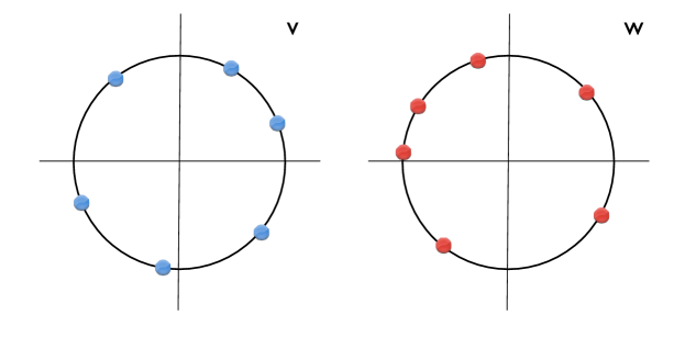
Figure 10.1: Statistical dual of non-BPS brane: blue and red dots represent charges with $Q_{+}=1$ and $Q_{-}=-1$, respectively.

Let us suppose that this system is immersed into a heat bath at inverse temperature $\beta=1/T$. We can then aim to make contact with the disk partition function, by moving to consider the grand canonical ensemble with a particle reservoir with chemical potentials $\mu_{+},\mu_{-}$. The grand canonical partition function of this system will then be

$$Z_{G} = \sum_{N_{+}=N_{-}}\left[\frac{{z_{+}}^{N_{+}}}{N_{+}!}\int_{0}^{2\pi}\prod_{i=1}^{N_{+}}\frac{dt_{i}}{2\pi}\,e^{\left(-\beta\sum_{i<j}V^{\rm Dyson}(t_{i},t_{j})\right)}\right]$$ (10.9)

$$\qquad\qquad\left[\frac{{z_{-}}^{N_{-}}}{N_{-}!}\int_{0}^{2\pi}\prod_{i=1}^{N_{-}}\frac{d\tau_{i}}{2\pi}\,e^{\left(-\beta\sum_{k<l}V^{\rm Dyson}(\tau_{k},\tau_{l})\right)}\right]\ ,$$

where, as before, $V^{\rm Dyson}(x,y)=-\log|e^{ix}-e^{iy}|$. Here, $N_{\pm}!$ take into account that the system consists of identical particles of two types and $z_{\pm}=e^{\beta\mu_{\pm}}$ are the corresponding fugacities. At inverse temperature $\beta=2$ we then obtain

$$Z_{G}=\frac{1}{1-z_{+}z_{-}}\ .$$ (10.10)

Comparing (10.9) with the open string disk partition function calculation (10.6), by setting

$$z_{+}=-z_{-}=\pi\lambda e^{x^{0}/\sqrt{2}}\ ,$$ (10.11)

one finds

$$Z_{G}=\frac{1}{1+\pi^{2}\lambda^{2}e^{\sqrt{2}x^{0}}}=Z_{\rm open}\ .$$ (10.12)

However, we would like to avoid having complex chemical potentials. If we want to end up with positive fugacity $z_{-}$, a simple remedy is to insert a $(-)^{N}$ into the sum (10.6), and consider, instead of $Z_{\rm open}$, the quantity $Z^{\prime}_{\rm open}\equiv\langle i^{\hat{N}_{T}}\rangle_{\rm brane}$. The virtue of this is that it can be related to the grand canonical partition function with positive fugacities. Another way of achieving this is to analytically continue $z_{-}\to-z_{-}$, while keeping $\lambda$ positive, so that we have one-to-one correspondence with time $x^{0}$ of the decaying brane and a positive fugacity,

$$z\equiv|z_{+}|=|z_{-}|=\pi\lambda e^{x^{0}/\sqrt{2}}\ .$$ (10.13)

See Balasubramanian:2006sg for more extensive discussion on this issue.

10.3 Correlation Functions

To further establish the relation between the non-BPS brane and the paired Dyson gas, we also need to prescribe how to calculate the worldsheet correlation functions in the Dyson gas picture. For clarity, in this subsection we will explicitly write $z_{\pm}$ in favor of $z$.

10.3.1 NS-NS Vertex Operators

The statistical dual will correspond to inserting a set of test charges with charges $q_{+}^{a}=i\omega_{a}/\sqrt{2}$ at $v=z_{a}$ and another set of test charges with charges $q_{-}^{a}=-i\omega_{a}/\sqrt{2}$ at $w=z_{a}$.

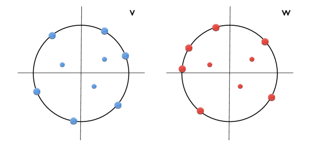
Figure 10.2: Statistical dual of NS-NS vertex operators insertion: smaller blue and red dots represent test charges with $q_{+}^{a}=i\omega_{a}/\sqrt{2}$ at $v=z_{a}$, and $q_{-}^{a}=-i\omega_{a}/\sqrt{2}$ at $w=z_{a}$, respectively.

To be more precise, let us consider inserting vertex operators in the form of

$$V_{s}=\prod_{a=1}^{n}e^{i\omega_{a}X^{0}(z_{a},\bar{z}_{a})}.$$ (10.14)

To compute the correlation functions of this kind in the Dyson gas picture, we need to compute the grand canonical “expectation value” of the quantity $e^{-\beta\,V^{\rm bulk}}$, where $V^{\rm bulk}$ is the interaction among bulk charges. This is defined as

$$\langle\prod_{a=1}^{n}e^{i\omega_{a}X^{0}(z_{a},\bar{z}_{a})}\rangle \equiv \sum_{N}\left(\frac{z_{+}^{N}}{N!}\int\prod_{i=1}^{N}\frac{dt_{i}}{2\pi}\,e^{\left[-\beta\left(V_{+}^{\rm Dyson}+V_{+}^{\rm bulk-Dyson}\right)\right]}\cdot e^{-\beta\,V_{+}^{\rm bulk}}\right)$$

$$\qquad\left(\frac{z_{-}^{N}}{N!}\int\prod_{i=1}^{N}\frac{d\tau_{i}}{2\pi}\,e^{\left[-\beta\left(V_{-}^{\rm Dyson}+V_{-}^{\rm bulk-Dyson}\right)\right]}\cdot e^{-\beta\,V_{-}^{\rm bulk}}\right),$$

where $V^{\rm bulk-Dyson}$ is the interaction between the bulk charges and the Dyson gas particles.

10.3.2 R-R Vertex Operators

For correlation functions involving R-R sector, we need to do two things:

• add $|k|$ Dyson particles with charges $Q={\rm sign(k)}$ to the respective two-dimensional plane (i.e., $Q=+1$ to $v$-plane, $Q=-1$ to $w$-plane). Here, $k$ is defined as $k\equiv-\sum_{a}(s_{a}+\tilde{s}_{a})\in\mathbb{Z}$;

• insert test charges with $q_{+}^{a}=(i\omega_{a}/\sqrt{2}+(s_{a}+\tilde{s}_{a})/2)$ at $v=z_{a}$, and $q_{-}^{a}=(-i\omega_{a}/\sqrt{2}+(s_{a}+\tilde{s}_{a})/2)$ at $w=z_{a}$, respectively.

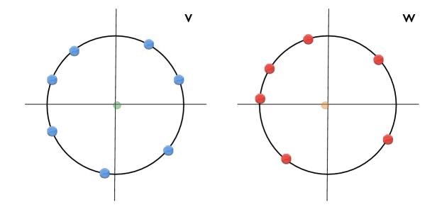
Figure 10.3: Statistical dual of R-R vertex operators insertion: green and orange dots represent test charges with $q_{+}^{a}=(i\omega_{a}/\sqrt{2}+(s_{a}+\tilde{s}_{a})/2)$ at $v=z_{a}$, and $q_{-}^{a}=(-i\omega_{a}/\sqrt{2}+(s_{a}+\tilde{s}_{a})/2)$ at $w=z_{a}$, respectively. Here, as an example, we have taken $s_{a}=\tilde{s}_{a}=1/2$ so that $k=1$. Thus, there is an extra $q=1$ Dyson particle on the boundary of $v$-disk.

Let us consider inserting vertex operators in the form of

$$\prod_{a=1}^{n}\Theta_{s_{a}}(z_{a})\tilde{\Theta}_{\tilde{s}_{a}}(\bar{z}_{a})\,e^{i\omega_{a}X^{0}(z_{a},\bar{z}_{a})}.$$ (10.16)

The prescription for calculating the expectation value in the Dyson gas picture then becomes

$$\langle\prod_{a=1}^{n}\Theta_{s_{a}}(z_{a})\tilde{\Theta}_{\tilde{s}_{a}}(\bar{z}_{a})e^{i\omega_{a}X^{0}(z_{a},\bar{z}_{a})}\rangle \equiv \sum_{N}\left(\frac{z_{+}^{N+|k|}}{(N+|k|)!}\int\prod_{i=1}^{N+|k|}\frac{dt_{i}}{2\pi}\,e^{\left[-\beta\left(V_{+}^{\rm Dyson}+V_{+}^{\rm bulk-Dyson}\right)\right]}\cdot\,e^{-\beta V_{+}^{\rm bulk}}\right)$$

$$\qquad\left(\frac{z_{-}^{N}}{N!}\int\prod_{i=1}^{N}\frac{d\tau_{i}}{2\pi}\,e^{\left[-\beta\left(V_{-}^{\rm Dyson}+V_{-}^{\rm bulk-Dyson}\right)\right]}\cdot e^{-\beta V_{-}^{\rm bulk}}\right)$$

for $k\geq 0$, or

$$\langle\prod_{a=1}^{n}\Theta_{s_{a}}(z_{a})\tilde{\Theta}_{\tilde{s}_{a}}(\bar{z}_{a})e^{i\omega_{a}X^{0}(z_{a},\bar{z}_{a})}\rangle \equiv \sum_{N}\left(\frac{z_{-}^{N+|k|}}{(N+|k|)!}\int\prod_{i=1}^{N+|k|}\frac{d\tau_{i}}{2\pi}\,e^{\left[-\beta\left(V_{-}^{\rm Dyson}+V_{-}^{\rm bulk-Dyson}\right)\right]}\cdot\,e^{-\beta V_{-}^{\rm bulk}}\right)$$

$$\qquad\left(\frac{z_{+}^{N}}{N!}\int\prod_{i=1}^{N}\frac{dt_{i}}{2\pi}\,e^{\left[-\beta\left(V_{+}^{\rm Dyson}+V_{+}^{\rm bulk-Dyson}\right)\right]}\cdot e^{-\beta V_{+}^{\rm bulk}}\right)$$

for $k\leq 0$.

[19pc] What then is time?
If no one asks me, I know what it is.
If I wish to explain it to him who asks, I do not know. Augustine of Hippo (354 - 430)

11 The Emergence of Time

The dualities between rolling tachyon backgrounds and Dyson gas systems, such as prescribed in the previous chapter, have been proven useful as tools for calculating observables in the rolling tachyon backgrounds Jokela:2008zh ; Jokela:2009zz ; Jokela:2009fd . However, these dualities are not only tools for calculation, they can also be thought of as reformulation of the unstable D-branes, which are K-theory objects and whose original descriptions include time, in terms of Dyson gas systems, which are statistical systems in thermal equilibrium that consist of objects without K-theory charges and whose descriptions do not include time.

In our present case of the paired Dyson gas picture, the time of the target spacetime $x^{0}$ has been replaced by the chemical potential $\mu$ of the statistical system. Different points of thermodynamic equilibrium characterized by different values of the chemical potential correspond to the different instants in time for the decaying non-BPS brane.

11.1 Time as the Average Particle Number

We can now give an interpretation to time as the average particle number in the statistical system. The average particle numbers for both sectors of the Dyson gases are

$$\bar{N}=\frac{z^{2}}{1-z^{2}}=\frac{\pi^{2}\lambda^{2}e^{\sqrt{2}x^{0}}}{1-\pi^{2}\lambda^{2}e^{\sqrt{2}x^{0}}}.$$ (11.1)

Solving for $x^{0}$ we get

$$x^{0}=\frac{1}{\sqrt{2}}\log\frac{\bar{N}}{1+\bar{N}}-\sqrt{2}\log\pi\lambda\ .$$ (11.2)

At the past infinity, $x^{0}\rightarrow-\infty$, we have vanishing fugacity and average particle number. Then $\bar{N}$ increases monotonically as a function of the fugacity corresponding to later time values of $x^{0}$.

$\bar{N}$, like time, is a continuous quantity. However, the underlying physical quantity is $N$, which is discrete. $N$ fluctuates around $\bar{N}$, and the fluctuation is given by

$$\frac{\delta N}{\bar{N}}=\frac{\sqrt{\langle N^{2}\rangle-\langle N\rangle^{2}}}{\bar{N}}=\frac{1}{z}=\frac{e^{-x^{0}/\sqrt{2}}}{\pi\lambda}\ .$$ (11.3)

At early times, $\delta N$ is large, but later $\bar{N}$ becomes more sharply defined. We can interpret this as a continuous time emerging from an underlying discrete variable $N$ in the large $N$ limit.

11.2 Thermodynamic Arrow of Time

Let us consider the grand potential of the statistical system

$$\Omega(z,T,V)=-T\log Z_{G}.$$ (11.4)

Using Legendre transformation, we can get the Helmholtz free energy

$$A(\bar{N},T,V)=-\frac{1}{2}\left[\log(\bar{N}+1)^{(\bar{N}+1)}-\log\bar{N}^{\bar{N}}\right].$$ (11.5)

We can then rewrite $A=-TI_{S}$ where $I_{S}$ is the Shannon entropy. Shannon entropy in the particle number distribution is given by

$$I_{S}=-\sum_{n}p(n)\log p(n);\,\,\,\,\,p(n)=\frac{(z^{2})^{n}}{Z_{G}},$$ (11.6)

where $p(n)$ is the probability that there are $n$ positively charged particles on $v$-disk and $n$ negatively charged particles on $w$-disk. Since $I_{s}$ increases as $\bar{N}$ increases, the free energy decrease as $\bar{N}$ increases. Recalling that the increase of $\bar{N}$ marks the passage of time, we can interpret this as a thermodynamic arrow of time.

[12pc] When will I learn? The answers to life’s problems aren’t at the bottom of a bottle, they’re on TV! Homer Simpson

12 Discussions

In this part of the thesis, we have reformulated the worldsheet description of non-BPS brane decay in terms of the statistical mechanics of the paired Dyson gas. As in the case of bosonic D-brane decay, the progress of time was marked by the increase of the average number of particles in the gas. The decrease of free energy marked the passage of time and thus gave rise to a thermodynamic arrow of time.

We would like to emphasize that even though one might have expected a non-equilibrium flow to realize the flow of time, this expectation is somewhat misleading. This is because there is already a physical time in non-equilibrium statistical mechanics. Thus, one can not expect to have time emerging from a non-equilibrium statistical mechanical system. Instead, in this set-up, we found that each instant of time was described by a different point of equilibrium in a statistical system.

In the known examples of emergence spatial dimensions, we learned that the classical or geometrical picture of spacetime is only valid in a certain limit. Here, we can also see that it is true, in the sense that the classical geometry of time, i.e., $\mathbb{R}$ emerges in the limit of large number of particles. Furthermore, we would also like to emphasize that this classical geometry of time does not correspond to a thermal state of the paired Dyson gas, but corresponds to the whole ensemble of the gas (c.f., black hole does not correspond to the thermal state but the whole ensemble of its microstates Balasubramanian:2007qv ).

If the notion of spacetime being emergent is true, then it is a possibility that spacetime symmetries are emergent too. In our case, the spacetime picture of the homogeneously decaying unstable D-brane is believed to be supersymmetric at late times, while on the other hand the Dyson gas is not. Then, one could ask whether the spacetime supersymmetry must be emergent too and how this is realized in Dyson gas language. This certainly deserves more study.

References

- (1) J. A. Hutasoit, “Vacuum Ambiguity in de Sitter Space at Strong Coupling,” JHEP 02 (2010) 026, arXiv:0910.5509 [hep-th].
- (2) J. A. Hutasoit, S. P. Kumar, and J. Rafferty, “Real time response on : the Topological AdS Black Hole and the Bubble,” JHEP 04 (2009) 063, arXiv:0902.1658 [hep-th].
- (3) J. A. Hutasoit and N. Jokela, “A Thermodynamic Interpretation of Time for Superstring Rolling Tachyons,” Phys. Rev. D77 (2008) 023521, arXiv:0709.1319 [hep-th].
- (4) J. M. Maldacena, “The large N limit of superconformal field theories and supergravity,” Adv. Theor. Math. Phys. 2 (1998) 231–252, arXiv:hep-th/9711200.
- (5) O. Aharony, S. S. Gubser, J. M. Maldacena, H. Ooguri, and Y. Oz, “Large N field theories, string theory and gravity,” Phys. Rept. 323 (2000) 183–386, arXiv:hep-th/9905111.
- (6) R.-G. Cai, “Constant curvature black hole and dual field theory,” Phys. Lett. B544 (2002) 176–182, arXiv:hep-th/0206223.
- (7) S. F. Ross and G. Titchener, “Time-dependent spacetimes in AdS/CFT: Bubble and black hole,” JHEP 02 (2005) 021, arXiv:hep-th/0411128.
- (8) V. Balasubramanian, K. Larjo, and J. Simon, “Much ado about nothing,” Class. Quant. Grav. 22 (2005) 4149–4170, arXiv:hep-th/0502111.
- (9) D. Birmingham and M. Rinaldi, “Bubbles in anti-de Sitter space,” Phys. Lett. B544 (2002) 316–320, arXiv:hep-th/0205246.
- (10) V. Balasubramanian and S. F. Ross, “The dual of nothing,” Phys. Rev. D66 (2002) 086002, arXiv:hep-th/0205290.
- (11) J. Polchinski, “String theory. Vol. 1: An introduction to the bosonic string,”. Cambridge, UK: Univ. Pr. (1998) 402 p.
- (12) J. Polchinski, “String theory. Vol. 2: Superstring theory and beyond,”. Cambridge, UK: Univ. Pr. (1998) 531 p.
- (13) T. Regge, “Introduction to complex orbital momenta,” Nuovo Cim. 14 (1959) 951.
- (14) T. Regge, “Bound states, shadow states and Mandelstam representation,” Nuovo Cim. 18 (1960) 947–956.
- (15) G. F. Chew and S. C. Frautschi, “PRINCIPLE OF EQUIVALENCE FOR ALL STRONGLY INTERACTING PARTICLES WITHIN THE S MATRIX FRAMEWORK,” Phys. Rev. Lett. 7 (1961) 394–397.
- (16) G. Veneziano, “Construction of a crossing - symmetric, Regge behaved amplitude for linearly rising trajectories,” Nuovo. Cim. A57 (1968) 190–197.
- (17) Y. Nambu, “DUAL MODEL OF HADRONS,”. EFI-70-07.
- (18) Z. Koba and H. B. Nielsen, “Reaction amplitude for n mesons: A Generalization of the Veneziano-Bardakci-Ruegg-Virasora model,” Nucl. Phys. B10 (1969) 633–655.
- (19) H. B. Nielsen and P. Olesen, “A Parton view on dual amplitudes,” Phys. Lett. B32 (1970) 203.
- (20) L. Susskind, “Dual symmetric theory of hadrons. 1,” Nuovo Cim. A69 (1970) 457–496.
- (21) J. Scherk and J. H. Schwarz, “Dual Models for Nonhadrons,” Nucl. Phys. B81 (1974) 118–144.
- (22) T. Yoneya, “Connection of Dual Models to Electrodynamics and Gravidynamics,” Prog. Theor. Phys. 51 (1974) 1907–1920.
- (23) J. Polchinski, “Dirichlet-Branes and Ramond-Ramond Charges,” Phys. Rev. Lett. 75 (1995) 4724–4727, arXiv:hep-th/9510017.
- (24) C. V. Johnson, “D-branes,”. Cambridge, USA: Univ. Pr. (2003) 548 p.
- (25) E. Witten, “D-branes and K-theory,” JHEP 12 (1998) 019, arXiv:hep-th/9810188.
- (26) P. Horava, “Type IIA D-branes, K-theory, and matrix theory,” Adv. Theor. Math. Phys. 2 (1999) 1373–1404, arXiv:hep-th/9812135.
- (27) H. Garcia-Compean, “D-branes in orbifold singularities and equivariant K- theory,” Nucl. Phys. B557 (1999) 480–504, arXiv:hep-th/9812226.
- (28) S. Gukov, “K-theory, reality, and orientifolds,” Commun. Math. Phys. 210 (2000) 621–639, arXiv:hep-th/9901042.
- (29) K. Hori, “D-branes, T-duality, and index theory,” Adv. Theor. Math. Phys. 3 (1999) 281–342, arXiv:hep-th/9902102.
- (30) E. R. Sharpe, “D-branes, derived categories, and Grothendieck groups,” Nucl. Phys. B561 (1999) 433–450, arXiv:hep-th/9902116.
- (31) K. Olsen and R. J. Szabo, “Brane descent relations in K-theory,” Nucl. Phys. B566 (2000) 562–598, arXiv:hep-th/9904153.
- (32) A. Sen, “Non-BPS states and branes in string theory,” arXiv:hep-th/9904207.
- (33) S. S. Gubser and A. Karch, “From gauge-string duality to strong interactions: a Pedestrian’s Guide,” Ann. Rev. Nucl. Part. Sci. 59 (2009) 145–168, arXiv:0901.0935 [hep-th].
- (34) R. A. Janik, “The dynamics of quark-gluon plasma and AdS/CFT,” arXiv:1003.3291 [hep-th].
- (35) S. A. Hartnoll, “Lectures on holographic methods for condensed matter physics,” Class. Quant. Grav. 26 (2009) 224002, arXiv:0903.3246 [hep-th].
- (36) J. McGreevy, “Holographic duality with a view toward many-body physics,” arXiv:0909.0518 [hep-th].
- (37) S. B. Giddings, S. Kachru, and J. Polchinski, “Hierarchies from fluxes in string compactifications,” Phys. Rev. D66 (2002) 106006, arXiv:hep-th/0105097.
- (38) A. M. Uranga, “The standard model in string theory from D-branes,” Nucl. Phys. Proc. Suppl. 171 (2007) 119–138.
- (39) C. P. Burgess, L. E. Ibanez, and F. Quevedo, “Strings at the intermediate scale or is the Fermi scale dual to the Planck scale?,” Phys. Lett. B447 (1999) 257–265, arXiv:hep-ph/9810535.
- (40) D. V. Gioutsos, G. K. Leontaris, and A. Psallidas, “D-brane standard model variants and split supersymmetry: Unification and fermion mass predictions,” Phys. Rev. D74 (2006) 075007, arXiv:hep-ph/0605187.
- (41) J. P. Conlon, D. Cremades, and F. Quevedo, “Kaehler potentials of chiral matter fields for Calabi-Yau string compactifications,” JHEP 01 (2007) 022, arXiv:hep-th/0609180.
- (42) R. Easther, B. R. Greene, W. H. Kinney, and G. Shiu, “Inflation as a probe of short distance physics,” Phys. Rev. D64 (2001) 103502, arXiv:hep-th/0104102.
- (43) R. Easther, B. R. Greene, W. H. Kinney, and G. Shiu, “Imprints of short distance physics on inflationary cosmology,” Phys. Rev. D67 (2003) 063508, arXiv:hep-th/0110226.
- (44) R. Easther, B. R. Greene, W. H. Kinney, and G. Shiu, “A generic estimate of trans-Planckian modifications to the primordial power spectrum in inflation,” Phys. Rev. D66 (2002) 023518, arXiv:hep-th/0204129.
- (45) C. P. Burgess, J. M. Cline, F. Lemieux, and R. Holman, “Are inflationary predictions sensitive to very high energy physics?,” JHEP 02 (2003) 048, arXiv:hep-th/0210233.
- (46) L. Cornalba and M. S. Costa, “Time-dependent orbifolds and string cosmology,” Fortsch. Phys. 52 (2004) 145–199, arXiv:hep-th/0310099.
- (47) A. Sen, “Tachyon dynamics in open string theory,” Int. J. Mod. Phys. A20 (2005) 5513–5656, arXiv:hep-th/0410103.
- (48) M. Headrick, S. Minwalla, and T. Takayanagi, “Closed string tachyon condensation: An overview,” Class. Quant. Grav. 21 (2004) S1539–S1565, arXiv:hep-th/0405064.
- (49) V. Balasubramanian, N. Jokela, E. Keski-Vakkuri, and J. Majumder, “A thermodynamic interpretation of time for rolling tachyons,” Phys. Rev. D75 (2007) 063515, arXiv:hep-th/0612090.
- (50) N. Jokela, E. Keski-Vakkuri, and J. Majumder, “Timelike Boundary Sine-Gordon Theory and Two-Component Plasma,” Phys. Rev. D77 (2008) 023523, arXiv:0709.1318 [hep-th].
- (51) S. Hellerman and I. Swanson, “Dimension-changing exact solutions of string theory,” JHEP 09 (2007) 096, arXiv:hep-th/0612051.
- (52) S. Hellerman and I. Swanson, “Cosmological unification of string theories,” JHEP 07 (2008) 022, arXiv:hep-th/0612116.
- (53) S. Hellerman and I. Swanson, “Charting the landscape of supercritical string theory,” Phys. Rev. Lett. 99 (2007) 171601, arXiv:0705.0980 [hep-th].
- (54) B. Craps, S. Sethi, and E. P. Verlinde, “A Matrix Big Bang,” JHEP 10 (2005) 005, arXiv:hep-th/0506180.
- (55) B. Craps, “Big bang models in string theory,” Class. Quant. Grav. 23 (2006) S849–S881, arXiv:hep-th/0605199.
- (56) M. Berkooz and D. Reichmann, “A short review of time dependent solutions and space-like singularities in string theory,” Nucl. Phys. Proc. Suppl. 171 (2007) 69–87, arXiv:0705.2146 [hep-th].
- (57) B. Craps, T. Hertog, and N. Turok, “Quantum Resolution of Cosmological Singularities using AdS/CFT,” arXiv:0712.4180 [hep-th].
- (58) A. Awad, S. R. Das, A. Ghosh, J.-H. Oh, and S. P. Trivedi, “Slowly Varying Dilaton Cosmologies and their Field Theory Duals,” Phys. Rev. D80 (2009) 126011, arXiv:0906.3275 [hep-th].
- (59) N. Iizuka and J. Polchinski, “A Matrix Model for Black Hole Thermalization,” JHEP 10 (2008) 028, arXiv:0801.3657 [hep-th].
- (60) N. Iizuka, T. Okuda, and J. Polchinski, “Matrix Models for the Black Hole Information Paradox,” JHEP 02 (2010) 073, arXiv:0808.0530 [hep-th].
- (61) B. D. Chowdhury and A. Virmani, “Modave Lectures on Fuzzballs and Emission from the D1-D5 System,” arXiv:1001.1444 [hep-th].
- (62) A. Strominger, “The dS/CFT correspondence,” JHEP 10 (2001) 034, arXiv:hep-th/0106113.
- (63) Y. Sekino and L. Susskind, “Census Taking in the Hat: FRW/CFT Duality,” Phys. Rev. D80 (2009) 083531, arXiv:0908.3844 [hep-th].
- (64) J. P. Conlon and F. Quevedo, “Kaehler moduli inflation,” JHEP 01 (2006) 146, arXiv:hep-th/0509012.
- (65) J. J. Blanco-Pillado et al., “Inflating in a better racetrack,” JHEP 09 (2006) 002, arXiv:hep-th/0603129.
- (66) R. Holman and J. A. Hutasoit, “Axionic inflation from large volume flux compactifications,” arXiv:hep-th/0603246.
- (67) J. R. Bond, L. Kofman, S. Prokushkin, and P. M. Vaudrevange, “Roulette inflation with Kaehler moduli and their axions,” Phys. Rev. D75 (2007) 123511, arXiv:hep-th/0612197.
- (68) R. Holman and J. A. Hutasoit, “Systematics of moduli stabilization, inflationary dynamics and power spectrum,” JHEP 08 (2006) 053, arXiv:hep-th/0606089.
- (69) T. W. Grimm, “Axion Inflation in Type II String Theory,” Phys. Rev. D77 (2008) 126007, arXiv:0710.3883 [hep-th].
- (70) M. Cicoli, C. P. Burgess, and F. Quevedo, “Fibre Inflation: Observable Gravity Waves from IIB String Compactifications,” JCAP 0903 (2009) 013, arXiv:0808.0691 [hep-th].
- (71) L. McAllister, E. Silverstein, and A. Westphal, “Gravity Waves and Linear Inflation from Axion Monodromy,” arXiv:0808.0706 [hep-th].
- (72) M. Badziak, “F-term uplifted racetrack inflation,” arXiv:1005.5537 [hep-th].
- (73) M. Alishahiha, E. Silverstein, and D. Tong, “DBI in the sky,” Phys. Rev. D70 (2004) 123505, arXiv:hep-th/0404084.
- (74) R. Bean, X. Chen, G. Hailu, S. H. H. Tye, and J. Xu, “Duality Cascade in Brane Inflation,” JCAP 0803 (2008) 026, arXiv:0802.0491 [hep-th].
- (75) C. P. Burgess, J. M. Cline, and M. Postma, “Axionic D3-D7 Inflation,” JHEP 03 (2009) 058, arXiv:0811.1503 [hep-th].
- (76) D. Baumann, A. Dymarsky, S. Kachru, I. R. Klebanov, and L. McAllister, “D3-brane Potentials from Fluxes in AdS/CFT,” arXiv:1001.5028 [hep-th].
- (77) O. Aharony, M. Fabinger, G. T. Horowitz, and E. Silverstein, “Clean time-dependent string backgrounds from bubble baths,” JHEP 07 (2002) 007, arXiv:hep-th/0204158.
- (78) E. Witten, “Instability of the Kaluza-Klein Vacuum,” Nucl. Phys. B195 (1982) 481.
- (79) R. C. Myers and M. J. Perry, “Black Holes in Higher Dimensional Space-Times,” Ann. Phys. 172 (1986) 304.
- (80) F. Dowker, J. P. Gauntlett, G. W. Gibbons, and G. T. Horowitz, “The Decay of magnetic fields in Kaluza-Klein theory,” Phys. Rev. D52 (1995) 6929–6940, arXiv:hep-th/9507143.
- (81) D. Astefanesei and G. C. Jones, “S-branes and (anti-)bubbles in (A)dS space,” JHEP 06 (2005) 037, arXiv:hep-th/0502162.
- (82) R. Emparan, “AdS/CFT duals of topological black holes and the entropy of zero-energy states,” JHEP 06 (1999) 036, arXiv:hep-th/9906040.
- (83) J. Alsup and G. Siopsis, “Low-lying quasinormal modes of topological AdS black holes and hydrodynamics,” Phys. Rev. D78 (2008) 086001, arXiv:0805.0287 [hep-th].
- (84) G. Koutsoumbas, E. Papantonopoulos, and G. Siopsis, “Discontinuities in Scalar Perturbations of Topological Black Holes,” Class. Quant. Grav. 26 (2009) 105004, arXiv:0806.1452 [hep-th].
- (85) G. Koutsoumbas, E. Papantonopoulos, and G. Siopsis, “Shear Viscosity and Chern-Simons Diffusion Rate from Hyperbolic Horizons,” Phys. Lett. B677 (2009) 74–78, arXiv:0809.3388 [hep-th].
- (86) M. Banados, “Constant curvature black holes,” Phys. Rev. D57 (1998) 1068–1072, arXiv:gr-qc/9703040.
- (87) M. Banados, A. Gomberoff, and C. Martinez, “Anti-de Sitter space and black holes,” Class. Quant. Grav. 15 (1998) 3575–3598, arXiv:hep-th/9805087.
- (88) M. Banados, M. Henneaux, C. Teitelboim, and J. Zanelli, “Geometry of the (2+1) black hole,” Phys. Rev. D48 (1993) 1506–1525, arXiv:gr-qc/9302012.
- (89) M. Banados, C. Teitelboim, and J. Zanelli, “The Black hole in three-dimensional space-time,” Phys. Rev. Lett. 69 (1992) 1849–1851, arXiv:hep-th/9204099.
- (90) S. W. Hawking and D. N. Page, “Thermodynamics of Black Holes in anti-De Sitter Space,” Commun. Math. Phys. 87 (1983) 577.
- (91) E. Witten, “Anti-de Sitter space and holography,” Adv. Theor. Math. Phys. 2 (1998) 253–291, arXiv:hep-th/9802150.
- (92) G. W. Gibbons and S. W. Hawking, “Cosmological Event Horizons, Thermodynamics, and Particle Creation,” Phys. Rev. D15 (1977) 2738–2751.
- (93) C. P. Herzog and D. T. Son, “Schwinger-Keldysh propagators from AdS/CFT correspondence,” JHEP 03 (2003) 046, arXiv:hep-th/0212072.
- (94) K. Skenderis and B. C. van Rees, “Real-time gauge/gravity duality,” Phys. Rev. Lett. 101 (2008) 081601, arXiv:0805.0150 [hep-th].
- (95) K. Skenderis and B. C. van Rees, “Real-time gauge/gravity duality: Prescription, Renormalization and Examples,” JHEP 05 (2009) 085, arXiv:0812.2909 [hep-th].
- (96) D. T. Son and A. O. Starinets, “Minkowski-space correlators in AdS/CFT correspondence: Recipe and applications,” JHEP 09 (2002) 042, arXiv:hep-th/0205051.
- (97) G. Policastro, D. T. Son, and A. O. Starinets, “From AdS/CFT correspondence to hydrodynamics,” JHEP 09 (2002) 043, arXiv:hep-th/0205052.
- (98) D. T. Son and A. O. Starinets, “Viscosity, Black Holes, and Quantum Field Theory,” Ann. Rev. Nucl. Part. Sci. 57 (2007) 95–118, arXiv:0704.0240 [hep-th].
- (99) G. T. Horowitz and E. Silverstein, “The inside story: Quasilocal tachyons and black holes,” Phys. Rev. D73 (2006) 064016, arXiv:hep-th/0601032.
- (100) E. Mottola, “Particle Creation in de Sitter Space,” Phys. Rev. D31 (1985) 754.
- (101) B. Allen, “Vacuum States in de Sitter Space,” Phys. Rev. D32 (1985) 3136.
- (102) T. S. Bunch and P. C. W. Davies, “Quantum Field Theory in de Sitter Space: Renormalization by Point Splitting,” Proc. Roy. Soc. Lond. A360 (1978) 117–134.
- (103) N. D. Birrell and P. C. W. Davies, “QUANTUM FIELDS IN CURVED SPACE,”. Cambridge, Uk: Univ. Pr. ( 1982) 340p.
- (104) U. H. Danielsson, “On the consistency of de Sitter vacua,” JHEP 12 (2002) 025, arXiv:hep-th/0210058.
- (105) H. Collins, R. Holman, and M. R. Martin, “The fate of the alpha-vacuum,” Phys. Rev. D68 (2003) 124012, arXiv:hep-th/0306028.
- (106) H. Collins, “A short introduction to the fate of the alpha-vacuum,” arXiv:hep-th/0312144.
- (107) M. B. Einhorn and F. Larsen, “Interacting quantum field theory in de Sitter vacua,” Phys. Rev. D67 (2003) 024001, arXiv:hep-th/0209159.
- (108) T. Banks and L. Mannelli, “De Sitter vacua, renormalization and locality,” Phys. Rev. D67 (2003) 065009, arXiv:hep-th/0209113.
- (109) M. K. Parikh, I. Savonije, and E. P. Verlinde, “Elliptic de Sitter space: dS/Z(2),” Phys. Rev. D67 (2003) 064005, arXiv:hep-th/0209120.
- (110) H. Collins and R. Holman, “Taming the alpha vacuum,” Phys. Rev. D70 (2004) 084019, arXiv:hep-th/0312143.
- (111) K. Goldstein and D. A. Lowe, “A note on alpha-vacua and interacting field theory in de Sitter space,” Nucl. Phys. B669 (2003) 325–340, arXiv:hep-th/0302050.
- (112) K. Goldstein and D. A. Lowe, “Real-time perturbation theory in de Sitter space,” Phys. Rev. D69 (2004) 023507, arXiv:hep-th/0308135.
- (113) M. B. Einhorn and F. Larsen, “Squeezed states in the de Sitter vacuum,” Phys. Rev. D68 (2003) 064002, arXiv:hep-th/0305056.
- (114) U. H. Danielsson, “Inflation, holography and the choice of vacuum in de Sitter space,” JHEP 07 (2002) 040, arXiv:hep-th/0205227.
- (115) B. C. van Rees, “Real-time gauge/gravity duality and ingoing boundary conditions,” Nucl. Phys. Proc. Suppl. 192-193 (2009) 193–196, arXiv:0902.4010 [hep-th].
- (116) V. Balasubramanian, P. Kraus, A. E. Lawrence, and S. P. Trivedi, “Holographic probes of anti-de Sitter space-times,” Phys. Rev. D59 (1999) 104021, arXiv:hep-th/9808017.
- (117) D. Berenstein, “Large N BPS states and emergent quantum gravity,” JHEP 01 (2006) 125, arXiv:hep-th/0507203.
- (118) U. Gursoy, S. A. Hartnoll, T. J. Hollowood, and S. P. Kumar, “Topology change and new phases in thermal N = 4 SYM theory,” JHEP 11 (2007) 020, arXiv:hep-th/0703100.
- (119) D. Berenstein, “Strings on conifolds from strong coupling dynamics, part I,” JHEP 04 (2008) 002, arXiv:0710.2086 [hep-th].
- (120) D. E. Berenstein and S. A. Hartnoll, “Strings on conifolds from strong coupling dynamics: quantitative results,” JHEP 03 (2008) 072, arXiv:0711.3026 [hep-th].
- (121) M. Gary, S. B. Giddings, and J. Penedones, “Local bulk S-matrix elements and CFT singularities,” Phys. Rev. D80 (2009) 085005, arXiv:0903.4437 [hep-th].
- (122) I. Heemskerk, J. Penedones, J. Polchinski, and J. Sully, “Holography from Conformal Field Theory,” JHEP 10 (2009) 079, arXiv:0907.0151 [hep-th].
- (123) S. D. Mathur, “Fuzzballs and the information paradox: a summary and conjectures,” arXiv:0810.4525 [hep-th].
- (124) V. Balasubramanian, J. de Boer, S. El-Showk, and I. Messamah, “Black Holes as Effective Geometries,” Class. Quant. Grav. 25 (2008) 214004, arXiv:0811.0263 [hep-th].
- (125) T. Hollowood, S. P. Kumar, and A. Naqvi, “Instabilities of the small black hole: A view from N = 4 SYM,” JHEP 01 (2007) 001, arXiv:hep-th/0607111.
- (126) E. Witten, “Anti-de Sitter space, thermal phase transition, and confinement in gauge theories,” Adv. Theor. Math. Phys. 2 (1998) 505–532, arXiv:hep-th/9803131.
- (127) A. Brandhuber, N. Itzhaki, J. Sonnenschein, and S. Yankielowicz, “Wilson loops, confinement, and phase transitions in large N gauge theories from supergravity,” JHEP 06 (1998) 001, arXiv:hep-th/9803263.
- (128) O. Aharony, J. Marsano, S. Minwalla, K. Papadodimas, and M. Van Raamsdonk, “The Hagedorn / deconfinement phase transition in weakly coupled large N gauge theories,” Adv. Theor. Math. Phys. 8 (2004) 603–696, arXiv:hep-th/0310285.
- (129) S. J. Avis, C. J. Isham, and D. Storey, “Quantum Field Theory in anti-De Sitter Space-Time,” Phys. Rev. D18 (1978) 3565.
- (130) L. D. Landau and E. M. Lifshitz, Fluid Mechanics. Oxford: Pergamon Press, 1987.
- (131) M. Spradlin, A. Strominger, and A. Volovich, “Les Houches lectures on de Sitter space,” arXiv:hep-th/0110007.
- (132) S. A. Hartnoll and S. Prem Kumar, “AdS black holes and thermal Yang-Mills correlators,” JHEP 12 (2005) 036, arXiv:hep-th/0508092.
- (133) P. Kovtun, M. Unsal, and L. G. Yaffe, “Volume independence in large N(c) QCD-like gauge theories,” JHEP 06 (2007) 019, arXiv:hep-th/0702021.
- (134) M. Unsal and L. G. Yaffe, “Center-stabilized Yang-Mills theory: confinement and large volume independence,” Phys. Rev. D78 (2008) 065035, arXiv:0803.0344 [hep-th].
- (135) L. Fidkowski, V. Hubeny, M. Kleban, and S. Shenker, “The black hole singularity in AdS/CFT,” JHEP 02 (2004) 014, arXiv:hep-th/0306170.
- (136) G. Festuccia and H. Liu, “Excursions beyond the horizon: Black hole singularities in Yang-Mills theories. I,” JHEP 04 (2006) 044, arXiv:hep-th/0506202.
- (137) C. Csaki, H. Ooguri, Y. Oz, and J. Terning, “Glueball mass spectrum from supergravity,” JHEP 01 (1999) 017, arXiv:hep-th/9806021.
- (138) http://functions.wolfram.com/.
- (139) M. Abramowitz and I. A. Stegun, Handbook of Mathematical Functions with Formulas, Graphs, and Mathematical Tables. Dover Publications, New York, NY, USA, 1964.
- (140) A. Karch and A. O’Bannon, “Chiral transition of N = 4 super Yang-Mills with flavor on a 3-sphere,” Phys. Rev. D74 (2006) 085033, arXiv:hep-th/0605120.
- (141) C. P. Herzog, A. Karch, P. Kovtun, C. Kozcaz, and L. G. Yaffe, “Energy loss of a heavy quark moving through N = 4 supersymmetric Yang-Mills plasma,” JHEP 07 (2006) 013, arXiv:hep-th/0605158.
- (142) J. A. Hutasoit and J. Rafferty work in progress .
- (143) J. Polchinski, “S-matrices from AdS spacetime,” arXiv:hep-th/9901076.
- (144) R. Bousso, A. Maloney, and A. Strominger, “Conformal vacua and entropy in de Sitter space,” Phys. Rev. D65 (2002) 104039, arXiv:hep-th/0112218.
- (145) N. Seiberg, “Emergent spacetime,” arXiv:hep-th/0601234.
- (146) I. R. Klebanov, “String theory in two-dimensions,” arXiv:hep-th/9108019.
- (147) W. Taylor, “M(atrix) theory: Matrix quantum mechanics as a fundamental theory,” Rev. Mod. Phys. 73 (2001) 419–462, arXiv:hep-th/0101126.
- (148) M. Gutperle and A. Strominger, “Spacelike branes,” JHEP 04 (2002) 018, arXiv:hep-th/0202210.
- (149) A. Sen, “Rolling Tachyon,” JHEP 04 (2002) 048, arXiv:hep-th/0203211.
- (150) A. Sen, “Tachyon matter,” JHEP 07 (2002) 065, arXiv:hep-th/0203265.
- (151) F. Larsen, A. Naqvi, and S. Terashima, “Rolling tachyons and decaying branes,” JHEP 02 (2003) 039, arXiv:hep-th/0212248.
- (152) A. Sen, “Time and tachyon,” Int. J. Mod. Phys. A18 (2003) 4869–4888, arXiv:hep-th/0209122.
- (153) E. Witten, “Duality relations among topological effects in string theory,” JHEP 05 (2000) 031, arXiv:hep-th/9912086.
- (154) G. W. Moore and E. Witten, “Self-duality, Ramond-Ramond fields, and K-theory,” JHEP 05 (2000) 032, arXiv:hep-th/9912279.
- (155) D.-E. Diaconescu, G. W. Moore, and E. Witten, “A derivation of K-theory from M-theory,” arXiv:hep-th/0005091.
- (156) P. Horava, “Stability of Fermi surfaces and K-theory,” Phys. Rev. Lett. 95 (2005) 016405, arXiv:hep-th/0503006.
- (157) A. Kitaev, “Periodic table for topological insulators and superconductors,” AIP Conf. Proc. 1134 (2009) 22–30, arXiv:0901.2686 [cond-mat.mes-hall].
- (158) N. D. Lambert, H. Liu, and J. M. Maldacena, “Closed strings from decaying D-branes,” JHEP 03 (2007) 014, arXiv:hep-th/0303139.
- (159) J.-c. Hwang and E. T. Vishniac, “Gauge-invariant joining conditions for cosmological perturbations,” Astrophys. J. 382 (1991) 363–368.
- (160) N. Jokela, E. Keski-Vakkuri, and J. Majumder, “On superstring disk amplitudes in a rolling tachyon background,” Phys. Rev. D73 (2006) 046007, arXiv:hep-th/0510205.
- (161) J. Shelton, “Closed superstring emission from rolling tachyon backgrounds,” JHEP 01 (2005) 037, arXiv:hep-th/0411040.
- (162) V. Balasubramanian, E. Keski-Vakkuri, P. Kraus, and A. Naqvi, “String scattering from decaying branes,” Commun. Math. Phys. 257 (2005) 363–394, arXiv:hep-th/0404039.
- (163) N. Jokela, M. Jarvinen, and E. Keski-Vakkuri, “N-point functions in rolling tachyon background,” Phys. Rev. D79 (2009) 086013, arXiv:0806.1491 [hep-th].
- (164) N. Jokela, “String scattering amplitudes from Dyson gas,” Nucl. Phys. Proc. Suppl. 192-193 (2008) 146–147.
- (165) N. Jokela, M. Jarvinen, and E. Keski-Vakkuri, “Electrostatics approach to closed string pair production from a decaying D-brane,” Phys. Rev. D80 (2009) 126010, arXiv:0911.0339 [hep-th].
- (166) V. Balasubramanian et al., “Typicality versus thermality: An analytic distinction,” Gen. Rel. Grav. 40 (2008) 1863–1890, arXiv:hep-th/0701122.