Efficient decomposition of cosmic microwave background polarization maps into pure E, pure B, and ambiguous components

Abstract

Separation of the B component of a cosmic microwave background (CMB) polarization map from the much larger E component is an essential step in CMB polarimetry. For a map with incomplete sky coverage, this separation is necessarily hampered by the presence of “ambiguous” modes which could be either E or B modes. I present an efficient pixel-space algorithm for removing the ambiguous modes and separating the map into “pure” E and B components. The method, which works for arbitrary geometries, does not involve generating a complete basis of such modes and scales the cube of the number of pixels on the boundary of the map.

I Introduction

A great deal of attention in cosmology is focused on attempts to characterize the polarization of the cosmic microwave background (CMB) radiation. Multiple experiments have detected CMB polarization Leitch et al. (2005); Readhead et al. (2004); Page et al. (2007); Jones et al. (2006); Bischoff et al. (2008); Brown et al. (2009). The Planck Surveyor Delabrouille (2004) will provide all-sky polarization maps at many frequencies, and many other experiments are in development. Many in the cosmology community regard the quest for high-quality CMB polarization maps as an extremely high priority Bock et al. (2006); Dodelson et al. (2009). CMB polarization maps can potentially provide a great deal of information about our Universe, complementing the wealth of information provided by CMB temperature anisotropy.

Although polarization maps have multiple uses, much of the interest in CMB polarization stems from the prediction that a stochastic background of gravitational waves, prouced during an inflationary epoch, may be visible in polarization maps. Detection of this background would be of revolutionary importance, providing direct confirmation of inflation as well as a measurement of the inflation energy scale.

The possibility of detecting this gravitational wave background is a consequence of the fact that a CMB polarization map can be regarded as a sum of two components, a scalar $E$ component and a pseudoscalar $B$ component Kamionkowski et al. (1997a); Seljak and Zaldarriaga (1997); Zaldarriaga and Seljak (1997); Kamionkowski et al. (1997b). To linear order in perturbation theory, “ordinary” scalar perturbations populate only the $E$ component. The tensorial gravitational waves, on the other hand, populate both $E$ and $B$ components. Because the tensor component is known to be smaller in amplitude than the scalar component, detection of it requires a channel that is free of scalar contributions. $B$-component polarization may provide this channel.

The $B$ component is predicted to be at least an order of magnitude smaller than the $E$ component on all angular scales. It is therefore important to make sure that any detection of $B$-type polarization is free from contamination from the $E$ component. Such contamination can be caused by systematic errors, of course Hu et al. (2003); Bunn (2007); Shimon et al. (2008); O’Dea et al. (2007), but even in an error-free map one must worry about mixing of $E$ and $B$ components in the data analysis process Bunn (2002). For a map with complete sky coverage, the two components can be perfectly separated in the spherical harmonic domain, but for a map with only partial sky coverage care must be taken to separate components in a leakage-free way Lewis (2003); Lewis et al. (2002); Bunn et al. (2003); Bunn (2003, 2008).

One way to think about this concern is in the language of the “pure” and “ambiguous” components of a polarization map Bunn et al. (2003). A “pure $E$” (resp. $B$) mode on the incomplete sky is one that can only have been produced by $E$-type (resp. $B$-type) polarization, while an ambiguous mode is one that could have been produced by either component. To be specific, a (not necessarily pure) $E$ (resp. $B$) mode ${\bf P}$ is one that satisfies a certain differential relationship ${\bf D}_{B}^{\dagger}\cdot{\bf P}=0$ (resp. ${\bf D}_{E}^{\dagger}\cdot{\bf P}=0$). Explicit forms for the differential operators ${\bf D}_{E,B}$ are given in Section II, and further details may be found in refs. Lewis et al. (2002); Bunn et al. (2003). An ambiguous mode is one that satisfies both conditions simultaneously. There are no modes satisfying both conditions on the complete sphere, but there on any domain consisting of only part of the sphere.

“Pure” $E$ (resp. $B$) modes are defined to be orthogonal to all $B$ (resp. $E$) modes, including the ambiguous modes. Explicit examples of pure and ambiguous modes may be found in ref. Bunn et al. (2003).

On the incomplete sky, the decomposition into $E$ and $B$ components is not unique, since there is no way to decide where to put the ambiguous modes. One way to illustrate this is to imagine working with a square patch of sky in the flat-sky approximation. The $E$-$B$ decomposition is trivial in Fourier space, so one could perform the decomposition by Fourier transforming, decomposing, and transforming back. Now imagine performing this set of operations after padding the observed map out to a larger size, inserting any values you like in the unobserved region. Different $E$/$B$ decompositions will result depending on how the padding is performed, all of which will match the data over the observed region. If all one has access to is the observed patch, there is no way to tell which if any of these is the “real” $E$/$B$ decomposition.

Although the $E/B$ decomposition is not unique for a partial sky map, the decomposition into pure $E$, pure $B$, and ambiguous components is unique Bunn et al. (2003). In practice, if the $E$ component dominates over the $B$ component as expected, the ambiguous modes will mostly contain information about $E$ modes, and a robust detection of $B$-type polarization must therefore be sought in the pure $B$ component. One consequence of this loss of $B$ information to ambiguous modes is a shift in the optimum tradeoff between sensitivity and sky coverage Bunn (2002): the optimum sky coverage for a $B$-type experiment is larger than would be found by a straightforward “Knox formula” Knox (1997).

The information loss due to ambiguous modes has two sources: incomplete sky coverage and pixelization Bunn et al. (2003). Pixelization ambiguity is essentially a consequence of aliasing of Fourier modes (working in the flat-sky approximation for simplicity). In a map with pixel size $L_{\rm pix}$, Fourier modes with wavevector components greater than the Nyquist frequency $k_{\rm Ny}=2\pi/L_{\rm pix}$ are aliased to modes of lower frequency. In the process, the wave vector $\vec{k}$ is mapped to a new vector with, generically, a completely different direction. The decomposition of a Fourier mode into $E$ and $B$ components depends entirely on the direction of $\vec{k}$, so aliasing thoroughly scrambles $E$ and $B$ modes. There is only one way to avoid this: one must pixelize finely, pushing the Nyquist frequency to a level where beam suppression makes aliasing negligible.

If a data set has been pixelized too coarsely, resulting in significant aliasing, no data analysis method can undo the $E$-$B$ mixing. Therefore, in this paper, I will assume that the data have been sufficiently finely pixelized (relative to the beam size) to control pixelization-induced $E$-$B$ mixing to an acceptable level. The method described in this paper is aimed at removing the incomplete-sky-induced ambiguous component.

Of course, no matter how fine the pixelization, the noise will not be smooth on the pixel scale. Separate tests are therefore required to make sure that the decomposition described herein is well-behaved with respect to noise in the data. Section IV discusses such tests.

The original method for decomposition into pure E, pure B, and ambiguous components (hereinafter referred to as an E/B/A decomposition) involved the construction of an orthornormal basis of such modes by solution of an eigenvector problem of dimension $2N_{\rm pix}$, the number of pixels in the data set. Such an operation is computationally extremely expensive for large data sets. This paper will present an alternative algorithm that is far more efficient.

Even on an incomplete sky, it is easy to separate a polarization map into $E$ and $B$ components, if one does not worry about the purity of those components: one simply performs the operation in Fourier space (if the flat-sky approximation is appropriate) or spherical harmonic space; in either case the separation can be done mode by mode. The difficulty comes in projecting out the ambiguous component from each of these components. The ambiguous component of each map is determined by data on the boundary of the map, so it is natural to seek methods of finding it and projecting it out by examining only pixels near the boundary of the observed region. This paper will present one such method. As we will see, such methods can be far more efficient than the naïve method of finding a complete set of normal modes.

In principle, in order to perform power spectrum estimation (the primary goal of a CMB polarization experiment), it is not necessary to perform any E/B/A (or indeed E/B) separation at all. For any given choice of $E$ and $B$ power spectra, one can in principle compute the likelihood function $L(C_{l}^{E},C_{l}^{B})$ and use it to draw confidence intervals or Bayesian credible regions in power spectrum space. If this analysis excludes $C_{l}^{B}=0$, then $B$-type power has been detected. For large data sets, where the full likelihood is too expensive to compute, other methods such as the pseudo-$C_{l}$ method have been generalized from temperature anisotropy to polarization data Smith (2006a, b); Smith and Zaldarriaga (2007); Grain et al. (2009); Challinor and Chon (2005). Such methods achieve near-optimal power spectrum estimates without the need to perform an explicit E/B/A decomposition. There may well be other data analysis methods that do not involve worrying about an E/B/A decomposition. For example, one might analyze interferometric data entirely in visibility space Park and Ng (2004); Hamilton et al. (2008); Charlassier et al. (2010), without ever constructing a real-space map at all.

Nonetheless, E/B/A separation of polarization data sets will be useful for several reasons. Although the power spectra are the primary quantities to be measured in a CMB data set, they are not the end of the story; real-space maps are necessary for a variety of applications. Probably the most important will be tests for foreground contamination, which may be easier to do via real-space cross-correlation with foreground templates. Use of the lensing $B$-mode signal to constrain cosmological parameters (e.g., Kaplinghat et al. (2003); Smith et al. (2004); Lesgourgues et al. (2006)) depends on real-space $B$-component information, rather than just the power spectra. Searches for non-Gaussianity and departures from statistical isotropy also go beyond the power spectrum. A real-space picture of the pure $B$ component will be an important “sanity check” to make sure that the detected $B$ component looks qualitatively as expected. Last but certainly not least, people (both scientists and the broader public) will find it much easier to believe that $B$ modes have really been detected if there is an actual map they can be shown.

Other methods have been proposed for performing $E$-$B$ separation on incomplete sky maps Kim and Naselsky (2010); Zhao and Baskaran (2010); Cao and Fang (2009); Bowyer et al. (2011). These methods may prove extremely useful, but the method I propose herein differs from them in significant ways: it allows reconstruction of the actual polarization map components (i.e., the observables $Q,U$) as opposed to a scalar derivative of these quantities, and it does so by solving the relevant differential equation for the ambiguous modes, rather than by making a heuristic approximation that the ambiguous modes can be regarded as confined to the boundary of the map.

The remainder of this paper is organized as follows. Section II reviews the formalism behind pure and ambiguous components and lays out the schematic recipe for the E/B/A separation. Section III describes the technical details of the implementation. Section IV describes some tests of the algorithm, and Section V contains a brief discussion.

II Separation into pure and ambiguous modes

II.1 Review of formalism

We begin with a review of some useful relations involving $E$ and $B$ modes. The reader wishing further detail can see, e.g., refs. Lewis et al. (2002); Bunn et al. (2003). For simplicity, we work in the flat-sky approximation. Section V discusses the generalization to the spherical sky.

Let $Q(\vec{r})$ and $U(\vec{r})$ be the Stokes parameters as functions of position $\vec{r}$ on the sky. We will group them together into a vector field

$$\mathbf{p}=\begin{pmatrix}Q\\ U\end{pmatrix}.$$ (1)

Here and throughout, arrows denote spatial vectors, while boldface denotes vectors in more general vector spaces. In particular, $\mathbf{p}$ is not a vector in position space – i.e., it transforms with spin two rather than one.

For the present we neglect pixelization effects and allow ourselves to take derivatives. A polarization field is an E mode if it satisfies a second-order differential relation

$$\mathbf{D}_{B}^{\dagger}\cdot\mathbf{p}=0,$$ (2)

and is a B mode if it satisfies

$$\mathbf{D}_{E}^{\dagger}\cdot\mathbf{p}=0.$$ (3)

In the flat-sky approximation, the differential operators in these equations can be written

$$\mathbf{D}_{E} = \begin{pmatrix}\partial_{x}^{2}-\partial_{y}^{2}\\ 2\partial_{x}\partial_{y}\end{pmatrix}$$ (4)

$$\mathbf{D}_{B} = \begin{pmatrix}-2\partial_{x}\partial_{y}\\ \partial_{x}^{2}-\partial_{y}^{2}\end{pmatrix}$$ (5)

These two operators are the spin-2 analogues of the divergence and curl respectively. They satisfy the following useful relations:

$$\mathbf{D}_{E}^{\dagger}\cdot\mathbf{D}_{B}=\mathbf{D}_{B}^{\dagger}\cdot\mathbf{D}_{E} = 0,$$ (6)

$$\mathbf{D}_{E}^{\dagger}\cdot\mathbf{D}_{E}=\mathbf{D}_{B}^{\dagger}\cdot\mathbf{D}_{B} = \nabla^{4}\equiv(\nabla^{2})^{2}.$$ (7)

When working on the sphere rather than the plane, the operators $\mathbf{D}_{E,B}$ take on a more complicated form, and the bilaplacian $\nabla^{4}$ is replaced by $\nabla^{2}(\nabla^{2}+2)$.

Just as with curl- and divergence-free vector fields, we can express $E$ and $B$ modes in terms of potentials: any polarization field $\mathbf{p}_{E}$ that satisfies the $E$ mode condition can be written as the derivative of a potential $\psi_{E}$, and similarly for any $B$ mode $\mathbf{p}_{B}$:

$$\mathbf{p}_{E} = \mathbf{D}_{E}\psi_{E},$$ (8)

$$\mathbf{p}_{B} = \mathbf{D}_{B}\psi_{B}.$$ (9)

An ambiguous mode, by definition, is one that simultaneously satisfies the requirements of both $E$ and $B$ modes. We can construct such modes by choosing a biharmonic potential $\psi$, i.e., one with

$$\nabla^{4}\psi=0.$$ (10)

Then both $\mathbf{D}_{E}\psi$ and $\mathbf{D}_{B}\psi$ will be ambiguous modes: equations (6) and (7), along with the biharmonicity condition, imply that both $\mathbf{D}_{B}^{\dagger}$ and $\mathbf{D}_{E}^{\dagger}$ yield zero when applied to these fields.

A “pure” $E$ mode is defined to be one that is orthogonal, over the observed region, to all $B$ modes (including the ambiguous modes). Since it is an $E$ mode, a pure $E$ mode can always be derived from a potential $\psi_{E}$ via equation (8), and in order to be pure the potential must satisfy both Dirchlet and Neumann boundary conditions on the boundary $\partial\Omega$ of the observed region:

$$\left.\psi_{E}\right|_{\partial\Omega}=\left.\vec{n}\cdot\nabla\psi_{E}\right|_{\partial\Omega}=0,$$ (11)

where $\vec{n}$ is normal to the boundary. There is a unique biharmonic function satisfying a given set of Dirichlet and Neumann boundary conditions. Subtracting off the biharmonic function that matches the boundary conditions of $\psi_{E}$ gives a unique way to “purify” a given E mode.

II.2 Schematic recipe for E/B/A decomposition

Suppose that we have a polarization field $\mathbf{p}$ observed over a region $\Omega$. If we ignore pixelization issues and assume that we can differentiate, then we can decompose the field into pure E, pure B, and ambiguous components as follows:

1. Decompose $\mathbf{p}$ into E and B components without worrying about purity, specifically by finding a pair of potentials $\psi_{E},\psi_{B}$ such that

   $$\mathbf{p}=\mathbf{D}_{E}\psi_{E}+\mathbf{D}_{B}\psi_{B}.$$ (12)

2. Find functions $\alpha_{E},\alpha_{B}$ that are biharmonic, i.e.,

   $$\nabla^{4}\alpha_{X}=0$$ (13)

   (where $X$ is either $E$ or $B$) and that match the potentials on the boundaries:

   $$\left.\alpha_{X}\right|_{\partial\Omega} = \left.\psi_{X}\right|_{\partial\Omega},$$ (14)

   $$\left.\vec{n}\cdot\nabla\alpha_{X}\right|_{\partial\Omega} = \left.\vec{n}\cdot\nabla\psi_{X}\right|_{\partial\Omega}.$$ (15)

3. “Purify” the potentials by defining

   $$\psi_{pE}=\psi_{E}-\alpha_{E},\qquad\psi_{pB}=\psi_{B}-\alpha_{B}.$$ (16)

4. Apply the differential operators to obtain the pure E, pure B, and ambiguous polarization fields:

   $$\mathbf{p}_{pE} = \mathbf{D}_{E}\psi_{pE}$$ (17)

   $$\mathbf{p}_{pB} = \mathbf{D}_{B}\psi_{pB}$$ (18)

   $$\mathbf{p}_{a} = \mathbf{D}_{E}\alpha_{E}+\mathbf{D}_{B}\alpha_{B}.$$ (19)

For pixelized data, we can follow a similar procedure, with appropriately defined differential operators. Of course, we then have to test whether the discretization has introduced significant errors.

III Implementation

The procedure described in the previous section is straightforward in principle, but to implement it numerically on a discretized grid requires some care. In this section I will describe this procedure in more detail. I begin with a summary of the key points. The reader with sufficient patience can then proceed to examine the technical details in the rest of the section.

Before embarking on the above recipe, we need to embed our data in a rectangular grid, regarded as satisfying periodic boundary conditions, suitable for discrete Fourier transforms. We will then apply the various differential operators in the Fourier domain. Since the observed data will cover only a portion of the grid, we must extend it into the unobserved region. This extension must be smooth in order to avoid artifacts near the boundaries when we differentiate.

The Fourier-space differential operators are exact for functions that are band limited below the Nyquist frequency. We assume that the pixelization is fine enough, compared to the experimental beam, that the intrinsic signal has negligible power above the Nyquist frequency. The smooth extension must be designed so that the extended data are also smooth enough on the pixel scale to have power spectra that become negligible well before the Nyquist scale. I describe one method for smoothly extending the data in Section III.1.

Once the data have been extended, we can begin the decomposition. Step 1 is straightforward to implement in the Fourier domain, since the E/B decomposition can be done mode by mode in Fourier space (Section III.2).

Next we must find biharmonic functions satisfying the required boundary conditions. This can be done, e.g., by relaxation methods, but another method appears to be more efficient. We seek a function $\alpha$ such that $\nabla^{4}\alpha=0$ within the observed region $\Omega$ and $\alpha$ satisfies certain boundary conditions on $\partial\Omega$. We can identify a set of “source” points $S$ outside of the observed region on which $\nabla^{4}\alpha$ is allowed to be nonzero. By solving a linear system, we find the values of $\nabla^{4}\alpha$ on $S$ such that, when the inverse bilaplacian operator $\nabla^{-4}$ is applied, the resulting $\alpha$ satisfies the required boundary conditions. The inverse bilaplacian is a simple convolution with a fixed kernel and is efficient to apply in the Fourier domain. Section III.3 supplies details.

This procedure completes step 3 in our recipe, and step 4 is then trivially implemented in the Fourier domain, as described in the very brief Section III.4.

III.1 Smooth extension of data

Suppose that we have a data set $\mathbf{p}_{\rm obs}$ defined on a subset of the pixels in our grid. We need to extend it smoothly to a field $\mathbf{p}$ that covers the entire grid and matches $\mathbf{p}_{\rm obs}$ where data exist.

There are no doubt many ways to achieve this goal. One choice would be to create a realization of a Gaussian random process, constrained to match the observed data. Smoothness of the extension can then be enforced by assigning a steeply declining power spectrum to the random process.

There is a well-established process Hoffman and Ribak (1991, 1992) for generating constrained realizations of Gaussian random fields. The process involves two steps: first, the mean field of the constrained random process is found, and then random fluctuations are generated about that mean field. For our present purposes, we can simply stop after the first step: the mean field matches the constraints and is in fact smoother than the typical realization, so it is better for our purpose.

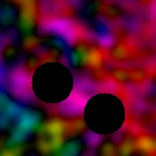
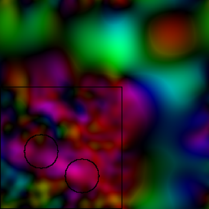
Figure 1: Illustration of maximum-likelihood extension. The upper left panel shows a simulated data set, observed over a square region with two holes in it. The direction of polarization is indicated by hue and the polarization amplitude by value in the HSV color system. The disc in the lower left illustrates this scheme, with polarization amplitude increasing with distance from the center and direction varying with angle. The data were simulated with power spectrum $P_{E}(k)\propto k^{-2}$ with no B modes, and smoothed with a Gaussian beam of width $\sigma=4$ pixels. The right panel shows the mean-field Gaussian extension of the data. The extension was calculated using a power spectrum $P(k)\propto k^{-4}$, with $P_{B}=0.01P_{E}$, and constrained to match the data over a 3-pixel boundary region.

We now describe this process in detail. Consider a Gaussian random process that generates a polarization map $\mathbf{g}=(Q,U)$, characterized by $E$ and $B$ mode power spectra $P_{E}(k),P_{B}(k)$. Suppose that the values of $\mathbf{g}$ are constrained to match $\mathbf{p}_{\rm obs}$ over the observed region, or at least over a subset of the observed region lying near the boundary. In practice, it is sufficient to choose to impose the constraint only on a band of pixels consisting of the $T_{\rm ext}$ nearest neighbors of boundary pixels, for some reasonably small $T_{\rm ext}$. We wish to determine the most probable realization of $\mathbf{g}$ on the rest of the pixels.

It is important to emphasize that the resulting $\mathbf{g}$ is not supposed to be the “real” polarization map extrapolated into the unobserved region. It is merely an artificial field designed solely to join smoothly onto the observed field. The power spectra $P_{E},P_{B}$ do not have to match those of the real data; in fact, it is better if they are very steeply declining, so that the Gaussian random process will strongly favor smooth functions.

Let the number of pixels in the entire grid be $N_{\rm pix}$ and the number of constraint pixels be $N_{\rm cons}$. Imagine writing the values of the Gaussian random field over the entire grid in a $2N_{\rm pix}$-dimensional vector $\mathbf{G}$. Some subset of these points are the $2N_{\rm cons}$ constraint values. These are listed in a $2N_{\rm cons}$-dimensional vector $\mathbf{C}$.

Let

$$\Xi_{ij}=\langle G_{i}G_{j}\rangle$$ (20)

be the correlation between any two elements of the (unconstrained) Gaussian random field. We use these values to define two matrices: $\mathbf{\Xi}^{cc}$ is the $2N_{\rm cons}\times 2N_{\rm cons}$ dimensional matrix giving the correlations between constraint points, and $\mathbf{\Xi}^{gc}$ is the $2N_{\rm pix}\times 2N_{\rm cons}$ dimensional matrix giving the correlations between arbitrary points and constraint points. Then the mean field, or most probable, value of $\mathbf{G}$ is

$$\mathbf{G}=\mathbf{\Xi}^{gc}\cdot(\mathbf{\Xi}^{cc})^{-1}\cdot\mathbf{C}.$$ (21)

Although this procedure sounds cumbersome, it is quite simple to apply. The covariance matrix elements $\Xi_{ij}$ are related in simple ways to the Fourier transforms of the power spectra $P_{E},P_{B}$. Moreover, they depend only on the vector separation between two pixels, which means that the multiplication by the matrix $\mathbf{\Xi}^{gc}$ in equation (21) is a convolution that can be done in time $N_{\rm pix}\ln N_{\rm pix}$. Calculation of the vector $(\mathbf{\Xi}^{cc})^{-1}\cdot\mathbf{C}$, on the other hand, requires time $O(N_{\rm cons}^{3})$. For a reasonably convex map with a “nice” boundary, the number of boundary pixels is of order the square root of the total number of pixels, in which case this is equivalent to $O(N_{\rm obs}^{3/2})$.

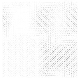
Figure 2: Numerical instability in extending maps. The original map (left panel) is a single B-type Fourier mode. It was extended using the mean-field method, with results shown in the center and right panels. The center panel shows the result of the extension when the Gaussian random process had no B power. The result is an attempt to match the input $B$ mode using only $E$ modes, leading to numerical instability: the maximum polarization level in the extended region is 590 times that of the original map, so that the original map (lower left quadrant) is invisible. The right panel shows the result obtained when $P_{B}$ is taken to be $0.01P_{E}$. In this case, the peak polarization level is 4.3 times that in the extended region.

Note that the computation of the $\mathbf{\Xi}$ matrices, as well as the Cholesky decomposition required on $\mathbf{\Xi}^{cc}$ depend only on the geometry of the system and are thus precomputable.

Figure 1 shows an example of this process. The “observed” region is a $150\times 150$ pixel patch with two circular holes 10 pixels in radius. The data consists of an E-type polarization field with a power spectrum $P_{E}(k)\propto k^{-2}$. (The simulation was made on a much larger $1200\times 1200$ grid and truncated, so that the observed grid does not satisfy periodic boundary conditions.) The observed region has been extended to a $256\times 256$ grid, including filling in the holes, following the procedure above. The extension was constrained to match the observed data over a boundary layer 3 pixels thick. The Gaussian random process assumed for the extension had both $P_{E}$ and $P_{B}$ proportional to $k^{-4}$ and $P_{B}=.01P_{E}$.

The extension smoothly joins onto the observed region and satisfies periodic boundary conditions, so that any further computations involving discrete Fourier transforms will be free of artifacts from discontinuities. Note that the extension becomes featureless far from the observed region. This simply reflects the fact that, when the constraints are unimportant, the most probable value of a Gaussian random process is uniformity.

Some choices must be made in applying this method, namely the thickness of the boundary layer on which to force matching, and the power spectra for both E and B modes in the Gaussian random process assumed for the extension. The choice of boundary layer thickness is governed by the desire for computational efficiency: if it does not lead to excessive computation time, there is no reason not to constrain on the entire observed region. However, since the purpose of the constraint is simply to insure smoothness of the extension, this is not necessary: numerical tests indicate that a boundary layer of a few pixels is sufficient.

The choice of power spectrum does not seem to make very much difference either, as long as it is a strongly decreasing function of $k$. I adopt a power-law power spectrum $P(k)\propto k^{-n_{s}}$, typically with $n_{s}=4$. The method can be applied with different power spectra for E and B modes. I recommend setting $P_{E}$ to be much larger than $P_{B}$, so that the extension will be nearly all E modes. This has the result that artifacts resulting from the extension will infect the pure E map more than the pure B map and thus do less damage. However, $P_{B}$ should not be taken to be zero: if the data set contains actual B modes, trying to satisfying the constraints with only E modes can lead to numerical instability as shown in Figure 2.

Section IV discusses some numerical tests on these parameters, showing that the final pure and ambiguous maps are insensitive to the choices made over a broad range.

III.2 Initial decomposition

After generating a smooth extension of the data onto a rectangular grid with periodic boundary conditions, decomposing the data into (impure) E and B components is trivial. We take discrete Fourier transforms of both $Q$ and $U$ and perform the decomposition mode by mode in the Fourier plane. For a given vector $\vec{k}$, making an angle $\alpha$ with the $x$ axis, an E mode would satisfy

$$\begin{pmatrix}\tilde{Q}_{E}\\ \tilde{U}_{E}\end{pmatrix}=\tilde{E}\begin{pmatrix}\cos 2\alpha\\ \sin 2\alpha\end{pmatrix}$$ (22)

for some ($\vec{k}$-dependent) scalar $\tilde{E}$, and similarly, a B mode would satify

$$\begin{pmatrix}\tilde{Q}_{B}\\ \tilde{U}_{B}\end{pmatrix}=\tilde{B}\begin{pmatrix}-\sin 2\alpha\\ \cos 2\alpha\end{pmatrix}.$$ (23)

We add these expressions, set the sum equal to $(\tilde{Q},\tilde{U})$, and solve:

$$\tilde{E} = \tilde{Q}\cos 2\alpha+\tilde{U}\sin 2\alpha,$$ (24)

$$\tilde{B} = -\tilde{Q}\sin 2\alpha+\tilde{U}\cos 2\alpha.$$ (25)

The fields $E$ and $B$ are the laplacians of the corresponding potentials $\psi_{E},\psi_{B}$, so in Fourier space,

$$\tilde{\psi}_{E}=-k^{-2}\tilde{E},\quad\tilde{\psi}_{B}=-k^{-2}\tilde{B}.$$ (26)

The monopole ($\vec{k}=0$) mode cannot be treated in this way, of course; it must be removed from the map and treated as an ambiguous mode. In addition, modes for which either $k_{x}$ or $k_{y}$ equals the Nyquist frequency must be treated with care: for such modes, we do not know the sign of one component of $k$, and hence do not know the quadrant of $\alpha$. This means that the terms proportional to $\sin 2\alpha$ in equations (24) and (25) have unknown sign. In the numerical implementation of this step, I separate these pieces and place them along with the monopole in the ambiguous component at the end of the process. Of course, the philosophy underlying the entire approach in this paper is that the Nyquist length is well below the smoothing scale, in which case this is always a minor consideration.

III.3 Solving the bilaplacian equation

We now consider the “purification” of $\psi_{E}$ and $\psi_{B}$. As we have seen, this step requires finding a biharmonic function $\alpha$ for each potential $\psi$ whose value and first derivative match the potential on the boundary. For efficiency’s sake, we wish to avoid method that require solution of linear systems of order $N_{\rm pix}$ dimensions.

One efficient method is to find $\beta=\nabla^{4}\alpha$ and then apply the inverse bilaplacian operator. We know that $\beta=0$ in the observed region, but it can (and indeed must) be nonzero for some unobserved pixels. We choose a set of $N_{\rm src}$ “source pixels,” all lying in the unobserved region, and allow $\beta$ to be nonzero only on these pixels. The boundary conditions are then a collection of $2N_{\rm bdy}$ linear equations to be solved for $N_{\rm src}$ unknowns. Generically, we expect solutions to exist if $N_{\rm src}\geq 2N_{\rm bdy}$.

Naturally, the solution we find will depend on the choice of source points, and even for a given set of source points, there will typically be multiple solutions. We might hope that all such solutions would coincide within the observed region, because of the uniqueness theorem for biharmonic functions. Unfortunately, this is not the case: the uniqueness theorem applies to functions whose boundary values and derivatives are specified at all boundary points, but we are imposing only a finite, discrete set of boundary conditions at the pixel locations. We must hope, therefore, that a judicious choice of source points and of solution to the linear system will yield a good approximation to the “correct” solution that we seek. In addition, of course, we must adopt criteria to judge whether we have succeeded.

It is plausible that the best choice of source points would be those lying near the boundary of the observed region. One way to see this is to note that the relation between $\beta$ and $\alpha$ is simply convolution with a fixed kernel: $\alpha=\nabla^{-4}\beta$ in real space, so that $\tilde{\alpha}=k^{-4}\tilde{\beta}$ in Fourier space. The real-space convolution kernel is shown in Figure 3. The kernel peaks at the source point and decays gradually. If we try to satisfy the boundary conditions using source points that are far away from the boundary, the sources will have to be quite large. Moreover, since each faraway source point will populate all of the boundary points to comparable levels, delicate cancellations of source points will be required. However, source points lying near the boundary will primarily populate their neighboring boundary points, which might plausibly lead to a more stable numerical system.

Based on this heuristic reasoning, I chose source points to lie in a boundary layer around the observed region, with the thickness $T_{\rm src}$ of the layer a free parameter. As the tests in the next section will show, this choice worked well. The primary errors arose in pixels right at the boundary. I therefore generalized the approach to consider source pixels that were offset from the boundary, i.e., those whose distance $d$ (in pixels) from the boundary lay in the interval $\Delta_{\rm src}\leq d<\Delta_{\rm src}+T_{\rm src}$, where the offset $\Delta_{\rm src}$ and the thickness $T_{\rm src}$ are both adjustable parameters.

Figure 3: Convolution kernel for the inverse bilaplacian. This graph shows the function $\alpha=\nabla^{-4}\beta$ in the case where $\beta$ is nonzero at only one pixel, lying at the center of the figure. For arbitrary $\beta$, $\alpha$ is obtained by convolution with this kernel.

The equations to be solved are in general underdetermined. One way to choose a solution in this case is to solve the system via singular value decomposition, which leads to the minimum-norm solution to a linear system. As we will see in the next section, a better solution is often obtained by retaining only some of the singular values in solving the system. The number of values to retain, $N_{\rm sing}$, is thus an additional adjustable parameter.

For a given choice of source points, the solution is straightforward to implement. The convolution kernel $K$ for the inverse bilaplacian is found in the pixel domain in $O(N_{\rm pix}\ln N_{\rm pix})$ time. If we then represent the linear system to be solved as a $2N_{\rm bdy}\times N_{\rm src}$ matrix $M$, then the matrix elements for the first $N_{\rm bdy}$ rows (corresponding to the Dirichlet boundary conditions) are of the form $M_{ij}=K(\vec{p}_{i}-\vec{q}_{j})$, where $\vec{p}_{i}$ is the location of the $i$th boundary pixel and $\vec{q}_{j}$ is the location of the $j$th source pixel. We can similarly compute the vector-valued kernel $\vec{K}_{g}$ for the gradient of the inverse bilaplacian, $\vec{\nabla}(\nabla^{-4})$. If $\hat{n}_{i}$ represents a unit normal to the boundary at the $i$th boundary pixel, then the lower half of the matrix $M$ (i.e., the rows corresponding to the Neumann boundary conditions) consists of elements of the form $\hat{n}_{i}\cdot\vec{K}_{g}(\vec{p}_{i}-\vec{q}_{j})$.

Extension	Power spectrum index	$n_{s}=4$
to unobserved	B to E power ratio	$P_{B}/P_{E}=0.01$
region	Boundary thickness (pixels)	$T_{\rm ext}=3$
Solving for	Source layer thickness (pixels)	$T_{\rm src}=10$
biharmonic	Source layer offset (pixels)	$\Delta_{\rm src}=1$
functions	Singular values retained	$N_{\rm sing}=600$

Table 1: Fiducial values for adjustable parameters in the E/B/A decomposition. The first three are used in extending the data into the unobserved region (Section III.1), and the last three are in solving the boundary-value problem for the ambiguous modes (Section III.3).

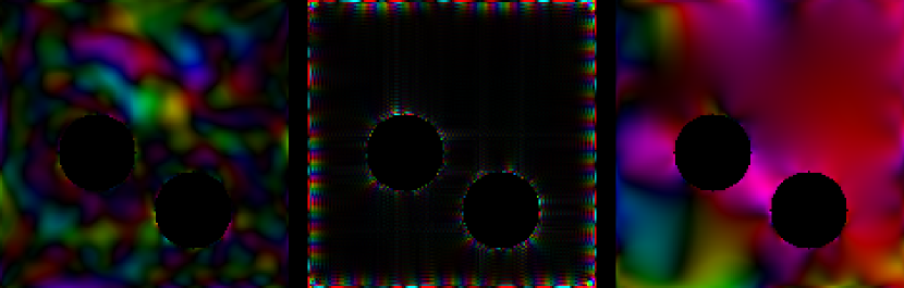
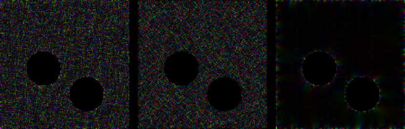
Figure 4: E/B/A decomposition. (a) The top panel shows the decomposition of the simulated map in Figure 1. The pure E, pure B, and ambiguous components are shown from left to right. The amplitude of the pure B component has been increased by a factor $10^{4}$. (b) The bottom panel shows the E/B/A decomposition of a pure white noise map. In this case, the B component is not increased in amplitude. In both cases, the fiducial parameters in Table 1 were used.

The most time-consuming step is the singular value decomposition, requiring $O(N_{\rm bdy}^{2}N_{\rm src})\sim O(T_{\rm src}N_{\rm bdy}^{3})$ time. Note, though, that this step depends only on the pixel geometry and can be precomputed.

Once the decomposition is performed, solving the linear system for any particular data set requires time $O(N_{\rm src}N_{\rm bdy})$. Using the result to populate $\alpha$ over the entire oberved region is done with a convolution, requiring $O(N_{\rm pix}\ln N_{\rm pix})$ time.

III.4 Constructing the pure and ambiguous maps.

Once the pure and ambiguous potentials have been found, it is straightforward to construct the final polarization maps by applying equations (17-19) in the Fourier domain. There is only one minor technical note. In the first step, we removed both the monopole and part of the Nyquist-frequency modes before passing from the original map to the potentials. We should add these terms into the ambiguous component at the end.

IV Tests

If we had continuously-sampled data and hence could take derivatives, the E/B/A decomposition would be unique and exact. The numerical method described in the previous section reduces to the exact decomposition in the limit where the pixelization becomes infinitely fine, but for pixelized data it is only approximate.

The Fourier-based derivative operators are exact for band-limited functions but approximate for functions with power above the Nyquist frequency. For (noise-free) data that are smoothed with a beam that is significantly larger than the pixel size, the intrinsic signal can be regarded as band-limited, to a good approximation. So can the Gaussian process that generates the extension. As long as the constraints imposed are sufficient to make these two maps join together smoothly, we expect, to a good approximation, to be able to regard the entire extended map as band-limited and hence differentiable in Fourier space.

Even in this case, the decomposition procedure is approximate, because the boundary conditions used to find the ambiguous modes are imposed only on a discrete set of boundary points, not continuously. Heuristically, we expect this to pose a problem chiefly on small scales, close to the pixel scale. As long as the data (including the extension into the unobserved region) have low power on scales close to the Nyquist scale, we can expect the method described above to work.

By construction, the pure $E$ (resp. $B$) component will be an $E$ (resp. $B$) mode – that is, the pure $E$ component will be a (sampled) derivative $\mathbf{D}_{E}$ of a band-limited potential, or equivalently it will be a discretization of a band-limited polarization field $\mathbf{p}_{pE}$ with $\mathbf{D}_{B}^{\dagger}\cdot\mathbf{p}_{pE}=0$. Similarly, the ambiguous component is by construction ambiguous, satisfying both $E$ and $B$ mode conditions. If the method fails, therefore, it will do so via a lack of purity of the supposedly pure components. This can be assessed by checking whether a map initially containing only $E$ modes has contamination in the pure $B$ component, and also by checking orthogonality of the three components

The above considerations apply to smooth data. Of course, the assumption of smoothness does not apply to noise in the data, so the question of how the decomposition acts on the noise is a very important one. For both signal and noise, the only way to know if the method is working is to perform numerical tests. Since the decomposition method is linear, we can measure its treatment of signal and noise separately.

Parameters	$B_{\rm max}$	$B_{\rm rms}$	$\xi_{\rm sig}$	$\xi_{\rm noise}$	$A_{\rm rms}^{\rm noise}$
Fiducial	$2.8\times 10^{-3}$	$5.5\times 10^{-5}$	1.0045	1.022	0.20
$P_{B}/P_{E}=0$	$2.5\times 10^{-4}$	$2.1\times 10^{-5}$	1.0045	1.21	0.39
$P_{B}/P_{E}=1$	$3.3\times 10^{-2}$	$4.2\times 10^{-4}$	1.0045	1.021	0.20
$P_{B}/P_{E}=100$	$6.5\times 10^{-2}$	$1.0\times 10^{-3}$	1.0045	1.021	0.19
$T_{\rm src}=5$	$8.0\times 10^{-3}$	$1.4\times 10^{-4}$	1.0045	1.019	0.19
$T_{\rm src}=2$	$2.6\times 10^{-2}$	$7.8\times 10^{-4}$	1.0060	1.018	0.19
$\Delta_{\rm src}=0$	$7.9\times 10^{-3}$	$1.5\times 10^{-4}$	1.0047	$1.018$	0.19
$N_{\rm sing}=100$	$0.10$	$9.3\times 10^{-2}$	1.020	1.28	0.51
$N_{\rm sing}=1800$	$7.5\times 10^{-4}$	$4.4\times 10^{-5}$	1.018	1.57	0.90

Table 2: Results of tests of the E/B/A decomposition algorithm. The quantities $B_{\rm rms}$ and $B_{\rm max}$ are the maximum and rms contamination of the pure B component, which should ideally be zero, as a fraction of the input rms power. The quantities $\xi_{\rm sig},\xi_{\rm noise}$, defined in equation (27), quantify the orthogonality of the three components in the signal and noise map respectively. Finally, $A_{\rm rms}^{\rm noise}$ is the noise rms found in the ambiguous component, as a fraction of the input noise rms. The first row shows results for the fiducial parameters of Table 1. In each subsequent row, one parameter is varied from the fiducial values.

The simulated map in Figure 1 (hereinafter referred to as the signal map) will be used to illustrate the performance of the method. The top panel of Figure 4 shows the result of applying the E/B/A decomposition procedure to this map. The decomposition method has a number of adjustable parameters, with the values listed in Table 1. The input map contained only $E$ modes, so the pure $B$ component should vanish. Note that the amplitude of this component has been increased by a factor $10^{4}$ simply to make it visible.

The bottom panel of Figure 4 shows an E/B/A decomposition of a map containing pure white noise, with the same observation geometry. In this case, one expects $E$ and $B$ to be comparable in amplitude, so the B component is not amplified.

To quantify the algorithm’s performance, I assess the following: the extent of contamination of the pure $B$ mode by $E$ power, the orthogonality of the three components, and the fraction of noise power in the ambiguous mode. The top line of Table 2 shows the results of these assessments. To quantify the contamination of the pure $B$ mode, I list both the maximum and the rms polarization amplitudes of the polarization in the pure $B$ map in Figure 4(a), compared to the rms amplitude of the input map. Since the contamination is highly concentrated near the boundary, the maximum is far larger than the rms, although it is still quite small.

To assess orthogonality of the pure $E$, pure $B$, and ambiguous components, I compute the total polarization power in each of the three components ($P\equiv\sum_{p}(Q_{p}^{2}+U_{p}^{2})$ over all pixels), as well as for the input map. I then compute

$$\xi=\sqrt{P_{pE}+P_{pB}+P_{a}\over P_{\rm input}},$$ (27)

which equals 1 if the three components are orthogonal and exceeds 1 if they are positively correlated. This quantity is computed for either the signal map or the noise map. The noise map provides a more stringent test, due to its abundance of high-frequency power.

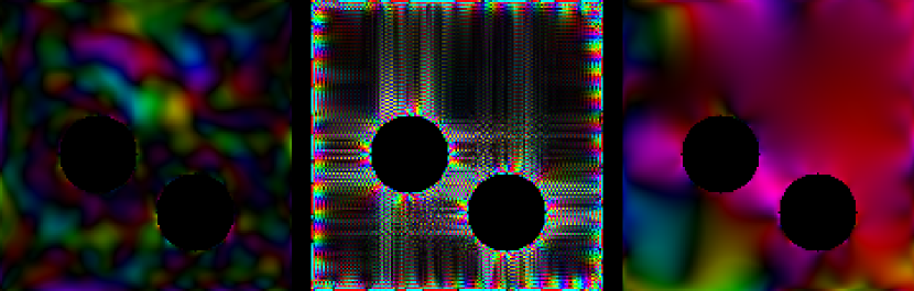
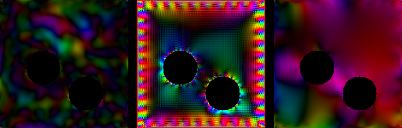
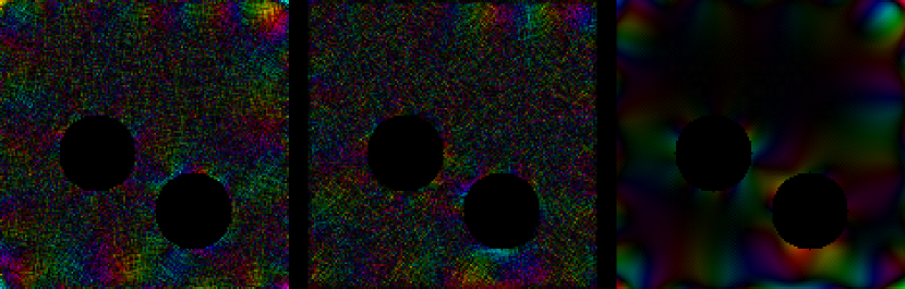
Figure 5: Effects of varying decomposition parameters. (a) The power spectrum index $n_{s}$ used for the extension is reduced from 4 to 2. (b) The number of source points used in finding biharmonic functions is reduced by setting the parameter $T_{\rm source}$ to 2. (c) The number of singular values retained in finding biharmonic functions is reduced to 100. Panels (a) and (b) show results for the simulated map of Figure 1, with the pure B component enhanced by a factor $10^{4}$ as in Figure 4. Panel (c) is for a white noise map, with no B enhancement.

Finally, the table lists the rms polarization amplitude in the ambiguous component of the noise map, relative to the rms input noise power. Once again, one could use either the simulated signal or the noise map in this assessment. The advantage of using the noise power is that we can predict approximately what we expect to see from simple considerations. The number of ambiguous modes below the Nyquist frequency is approximately equal to twice the length of the boundary in pixels Bunn et al. (2003). The total number of modes that can be measured is equal to twice the number of pixels. In a white-noise map, all orthonormal modes should have equal power, so the ratio of ambiguous-mode rms to total rms should be $\sqrt{N_{\rm bdy}/N_{\rm pix}}$. The number of boundary pixels in our case is $N_{\rm bdy}=932$, and the number of observed pixels is $N_{\rm pix}=19986$, so we expect the ratio to be approximately $0.2$.

The results show low levels of contaminated power and near-orthogonality as desired, and a level of ambiguous power in the noise map quite close to the theoretical estimate.

The fiducial values in Table 1 were chosen by trial and error to yield good results for these and similar tests, although they are certainly not the result of a systematic optimization procedure. On the contrary, increasing some parameters ($T_{\rm ext},T_{\rm source}$ in particular) causes the test results continue to improve very modestly, at the cost of greater computation time. The optimal choice of parameters will of course depend on the details of the data set to be analyzed and on the tradeoff between computation time and accuracy.

Table 2 and Figure 5 show the results of varying some of these parameters. For example, varying the spectral index used in extending the data to $n_{s}=2$ causes the extension to be less smooth, resulting in high-frequency power leaking into the pure B component [Figure 5(a)]. Reducing the number of source points used to find the biharmonic functions also results in increased leakage [Figure 5(b).] In both cases, recall that the B component is increased by $10^{4}$ in amplitude to make it visible: as Table 2 indicates, the actual levels of contamination are still quite small.

The E/B/A decomposition algorithm treats E and B identically, except in the adoption of different power spectrum normalizations for E and B modes used in extending the data. The line in Table 2 showing the effect of adopting a power spectrum ratio $P_{B}/P_{E}=100$ illustrates this breaking of symmetry: as expected, there is more leakage into the pure B mode when the extension is heavily weighted towards B modes. Equivalently, the fiducial ratio of 0.01 results in more leakage from $B$ into $E$ than vice versa. The fiducial choice $P_{B}/P_{E}=0.01$ is based on the assumption that leakage from E into B is more of a concern than leakage from B into E. If it is deemed important to maintain E/B symmetry in the process, however, one can choose $P_{B}/P_{E}=1$. The resulting rms leakage in this case is still quite less than one part in $10^{3}$, although the peak contamination, near the edges, rises to a few percent.

Some poor parameter choices result in numerical errors that can be seen in the failure of the components to be orthogonal and in the excess power going into the ambiguous mode. In particular, as noted in Section III.1, forcing the B component power spectrum $P_{B}$ to be identically zero in the extension leads to numerical instability as the actual B modes are shoehorned into E power. Keeping too many singular values in solving for the biharmonic functions also leads to numerical instability, causing the ambiguous component to contain non-ambiguous modes [Figure 5(c)].

V Discussion

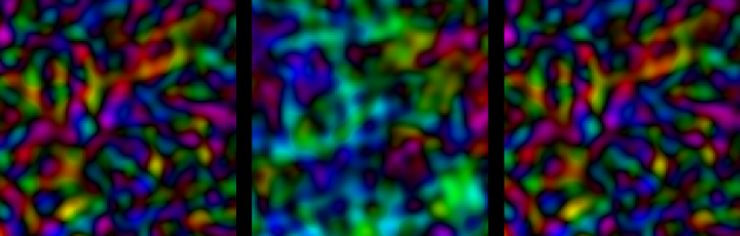
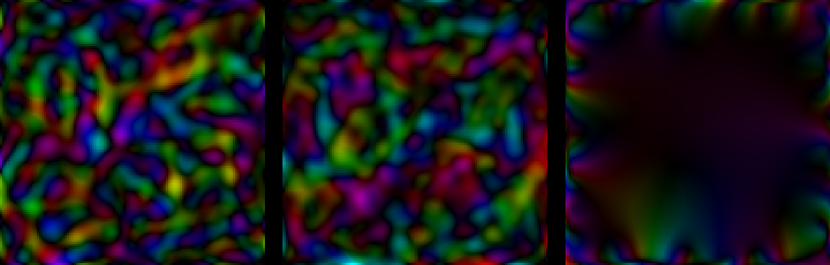
Figure 6: Illustration of E/B/A decomposition. The upper panel shows the $E$ component, $B$ component, and the sum of the two components for a simulated map based on a $\Lambda$CDM cosmological model with a tensor-scalar ratio $T/S=0.05$. The map contains $150\times 150$ pixels of size $3^{\prime}$ and was smoothed with a $\sigma=12^{\prime}$ beam. The $B$ component is enhanced by a factor 15 for visibility. The lower panel shows the result of the E/B/A decomposition: the pure $E$, pure $B$, and ambiguous components are shown from left to right. Again, the pure $B$ component is enhanced by a factor 15.

The tests in the previous section indicate that the methods described in this paper can give a good approximation to the pure E, pure B, and ambiguous modes of a CMB polarization data set. The components are close to orthogonal, and there is very low leakage of E modes into the pure B component. The leakage that does occur is, not surprisingly, close to the boundary of the observed region, where effects of boundary discretization are most important.

Figure 6 provides an additional illustration of the method, using more realistic input data than the simple power-low power spectra in previous examples. An input map was created containing both $E$ and $B$ modes, with power spectra computed by CAMB Lewis et al. (2000) based on the best-fit WMAP $\Lambda$CDM cosmology Komatsu et al. (2011), with a tensor-to-scalar ratio $T/S=0.05$. The simulated map is a $7.5^{\circ}\times 7.5^{\circ}$ square, pixelized into $150\times 150$ pixels $3^{\prime}$ in size. The map was smoothed with a $\sigma=12^{\prime}$ Gaussian beam. As in the previous example, the map was simulated on a larger $1200\times 1200$ grid and truncated, so that it would not have periodic boundary conditions. This map is sensitive to multipoles $30\lesssim l\lesssim 1000$.

The upper panel of Figure 6 shows the $E$ and $B$ components of the input map, as well as their sum. The lower panel shows the result of performing the E/B/A decomposition on the sum. In both cases, the $B$ component is enhanced by a factor 15 for visibility. The recovered $E$ and $B$ components look qualitatively similar to the input components, especially away from the edges. The pure $E$ component contains 81% of the input $E$ power ($Q^{2}+U^{2}$). The pure $B$ component contains 46% of the input $B$ power. The ambiguous component contains roughly 20% of the total power in the input map. As expected, nearly all of this ambiguous power comes from the $E$ component of the original map. The three components are very close to orthogonal: the quantity $\xi$ in equation (27) is $1.005$.

The method described in this paper was designed to avoid operations involving the solution of $N_{\rm pix}$-dimensional linear systems. The scaling of the various steps in the algorithm with data size is therefore of interest. Imagine a data set with $N_{\rm pix}$ pixels and a boundary of length $N_{\rm bdy}$ pixels. If the data set is reasonably round and has a smooth boundary, then we expect $N_{\rm bdy}\sim N_{\rm pix}^{1/2}$. (If the data are extremely “holey,” due, e.g., to the removal of many point sources, then $N_{\rm bdy}$ might be much larger. One might wish to search for special techniques for treating this particular case of many small round holes in the data.)

The smooth extension of the data involves the solution of a linear system of size $N_{\rm cons}\sim(T_{\rm ext}N_{\rm bdy})$, so the scaling of this step is $O((T_{\rm ext}N_{\rm bdy})^{3})\sim O(T_{\rm ext}^{3}N_{\rm pix}^{3/2})$, assuming a “nice” boundary. The most expensive step in the solution of this system is a Cholesky decomposition, which depends only on the pixel geometry and not on the data itself. Thus if multiple maps with the same geometry are to be analyzed (e.g., in Monte Carlo simulations), this step can be precomputed. The parts of the smooth extension that cannot be precomputed scale at most as $O(N_{\rm cons}^{2})$. (In any case, the method I have described for smooth extension is hardly unique; it is easy to imagine that faster ones can be found.)

The step involving the solution of the bilaplacian equation scales similarly: there is a precomputable singular value decomposition scaling as $O(N_{\rm bdy}^{2}N_{\rm src})\sim O(T_{\rm src}N_{\rm bdy}^{3})\sim O(T_{\rm src}N_{\rm pix}^{3/2})$, again assuming a “nice” boundary for the last step. The non-precomputable part of the process scales as $O(T_{\rm src}N_{\rm bdy}^{2})\sim O(T_{\rm src}N_{\rm pix})$.

The rest of the process involves Fourier transforms, which of course scale as $O(N_{\rm pix}\ln N_{\rm pix})$.

I have described and implemented the algorithm in the flat-sky approximation for simplicity. Each step in the process generalizes in a perfectly natural way to the spherical sky, so a spherical implementation should be perfectly possible. In this case, the Fourier transforms must be replaced with spherical harmonic transforms. The portions of the algorithm that scale as $N_{\rm pix}\ln N_{\rm pix}$ will then scale as $N_{\rm pix}^{3/2}$ (i.e., the same as the HEALPix Górski et al. (2005) programs synfast and anafast, and still at least as fast as the slowest other steps in the algorithm).

Alternative methods of performing an E/B/A decomposition have been proposed Kim and Naselsky (2010); Zhao and Baskaran (2010); Cao and Fang (2009). These methods are all potentially useful, but they differ from the one presented here in important ways. Some methods Kim and Naselsky (2010); Zhao and Baskaran (2010) involve finding scalar-valued derivatives of the pure components (essentially, $\mathbf{D}_{E,B}^{\dagger}\cdot\mathbf{p}$, but do not yield the actual polarization maps (i.e., Stokes $Q,U$) of the components. This has the advantage that the ambiguous contribution to the scalar maps is more concentrated at the boundary, so that approximate purification can be achieved by removing data near the edges. However, these methods do not allow for purification of the actual observables ($Q,U$), as for these quantities the ambiguous modes persist far into the interior (Figure 4). For some purposes, one may wish to analyze the pure $E$ and $B$ components of the actual polarization map.

In addition, there is a potentially promising method based on a wavelet decomposition Cao and Fang (2009). It too involves removing the ambiguous modes via a hard cutoff near the boundary, but the cutoff is set in terms of the scale of each wavelet, rather than being a fixed number of pixels. This is a sensible approach, as the distance an ambiguous mode persists into the interior of a map depends on the frequency of the source function on the boundary. In contrast, the method I have described does not make any a priori assumption about the ambiguous modes being restricted to the proximity of the border. Rather, it solves the relevant equation to determine how far from the border the ambiguous modes persist.

In preparing for the analysis of any particular data set, it would be extremely interesting to perform simulations to compare the performance of the various methods in detail.

References

- Leitch et al. (2005) E. M. Leitch, J. M. Kovac, N. W. Halverson, J. E. Carlstrom, C. Pryke, and M. W. E. Smith, Astrophys. J. 624, 10 (2005), eprint arXiv:astro-ph/0409357.
- Readhead et al. (2004) A. C. S. Readhead, S. T. Myers, T. J. Pearson, J. L. Sievers, B. S. Mason, C. R. Contaldi, J. R. Bond, R. Bustos, P. Altamirano, C. Achermann, et al., Science 306, 836 (2004), eprint arXiv:astro-ph/0409569.
- Page et al. (2007) L. Page, G. Hinshaw, E. Komatsu, M. R. Nolta, D. N. Spergel, C. L. Bennett, C. Barnes, R. Bean, O. Doré, J. Dunkley, et al., Astrophys. J. Supp. 170, 335 (2007), eprint arXiv:astro-ph/0603450.
- Jones et al. (2006) W. C. Jones, P. A. R. Ade, J. J. Bock, J. R. Bond, J. Borrill, A. Boscaleri, P. Cabella, C. R. Contaldi, B. P. Crill, P. de Bernardis, et al., New Astronomy Review 50, 945 (2006).
- Bischoff et al. (2008) C. Bischoff, L. Hyatt, J. J. McMahon, G. W. Nixon, D. Samtleben, K. M. Smith, K. Vanderlinde, D. Barkats, P. Farese, T. Gaier, et al., Astrophys. J. 684, 771 (2008), eprint 0802.0888.
- Brown et al. (2009) M. L. Brown, P. Ade, J. Bock, M. Bowden, G. Cahill, P. G. Castro, S. Church, T. Culverhouse, R. B. Friedman, K. Ganga, et al., Astrophys. J. 705, 978 (2009), eprint 0906.1003.
- Delabrouille (2004) J. Delabrouille, Astrophys. & Space Sci. 290, 87 (2004), eprint arXiv:astro-ph/0307549.
- Bock et al. (2006) J. Bock, S. Church, M. Devlin, G. Hinshaw, A. Lange, A. Lee, L. Page, B. Partridge, J. Ruhl, M. Tegmark, et al., ArXiv Astrophysics e-prints (2006), eprint arXiv:astro-ph/0604101.
- Dodelson et al. (2009) S. Dodelson, R. Easther, S. Hanany, L. McAllister, S. Meyer, L. Page, P. Ade, A. Amblard, A. Ashoorioon, C. Baccigalupi, et al., in astro2010: The Astronomy and Astrophysics Decadal Survey (2009), vol. 2010 of ArXiv Astrophysics e-prints, pp. 67–+, eprint 0902.3796.
- Kamionkowski et al. (1997a) M. Kamionkowski, A. Kosowsky, and A. Stebbins, Physical Review Letters 78, 2058 (1997a), eprint arXiv:astro-ph/9609132.
- Seljak and Zaldarriaga (1997) U. Seljak and M. Zaldarriaga, Physical Review Letters 78, 2054 (1997), eprint arXiv:astro-ph/9609169.
- Zaldarriaga and Seljak (1997) M. Zaldarriaga and U. Seljak, Phys. Rev. D 55, 1830 (1997), eprint arXiv:astro-ph/9609170.
- Kamionkowski et al. (1997b) M. Kamionkowski, A. Kosowsky, and A. Stebbins, Phys. Rev. D 55, 7368 (1997b), eprint arXiv:astro-ph/9611125.
- Hu et al. (2003) W. Hu, M. M. Hedman, and M. Zaldarriaga, Phys. Rev. D 67, 043004 (2003), eprint arXiv:astro-ph/0210096.
- Bunn (2007) E. F. Bunn, Phys. Rev. D 75, 083517 (2007), eprint arXiv:astro-ph/0607312.
- Shimon et al. (2008) M. Shimon, B. Keating, N. Ponthieu, and E. Hivon, Phys. Rev. D 77, 083003 (2008), eprint 0709.1513.
- O’Dea et al. (2007) D. O’Dea, A. Challinor, and B. R. Johnson, M.N.R.A.S. 376, 1767 (2007), eprint arXiv:astro-ph/0610361.
- Bunn (2002) E. F. Bunn, Phys. Rev. D 66, 069902 (2002).
- Lewis (2003) A. Lewis, Phys. Rev. D 68, 083509 (2003), eprint arXiv:astro-ph/0305545.
- Lewis et al. (2002) A. Lewis, A. Challinor, and N. Turok, Phys. Rev. D 65, 023505 (2002), eprint arXiv:astro-ph/0106536.
- Bunn et al. (2003) E. F. Bunn, M. Zaldarriaga, M. Tegmark, and A. de Oliveira-Costa, Phys. Rev. D 67, 023501 (2003), eprint arXiv:astro-ph/0207338.
- Bunn (2003) E. F. Bunn, New Astronomy Review 47, 987 (2003), eprint arXiv:astro-ph/0306003.
- Bunn (2008) E. F. Bunn, ArXiv e-prints (2008), eprint 0811.0111.
- Knox (1997) L. Knox, Astrophys. J. 480, 72 (1997), eprint arXiv:astro-ph/9606066.
- Smith (2006a) K. M. Smith, Phys. Rev. D 74, 083002 (2006a), eprint arXiv:astro-ph/0511629.
- Smith (2006b) K. M. Smith, New Astron. Rev. 50, 1025 (2006b), eprint arXiv:astro-ph/0608662.
- Smith and Zaldarriaga (2007) K. M. Smith and M. Zaldarriaga, Phys. Rev. D 76, 043001 (2007), eprint arXiv:astro-ph/0610059.
- Grain et al. (2009) J. Grain, M. Tristram, and R. Stompor, Phys. Rev. D 79, 123515 (2009), eprint 0903.2350.
- Challinor and Chon (2005) A. Challinor and G. Chon, M.N.R.A.S. 360, 509 (2005), eprint arXiv:astro-ph/0410097.
- Park and Ng (2004) C. Park and K. Ng, Astrophys. J. 609, 15 (2004), eprint arXiv:astro-ph/0304167.
- Hamilton et al. (2008) J. Hamilton, R. Charlassier, C. Cressiot, J. Kaplan, M. Piat, and C. Rosset, Astron. Astrophys. 491, 923 (2008), eprint 0807.0438.
- Charlassier et al. (2010) R. Charlassier, E. F. Bunn, J. Hamilton, J. Kaplan, and S. Malu, Astron. Astrophys. 514, A37+ (2010), eprint 0910.1864.
- Kaplinghat et al. (2003) M. Kaplinghat, L. Knox, and Y.-S. Song, Phys. Rev. Lett. 91, 241301 (2003).
- Smith et al. (2004) K. M. Smith, W. Hu, and M. Kaplinghat, Phys. Rev. D 70, 043002 (2004).
- Lesgourgues et al. (2006) J. Lesgourgues, L. Perotto, S. Pastor, and M. Piat, Phys. Rev. D 73, 045021 (2006).
- Kim and Naselsky (2010) J. Kim and P. Naselsky, ArXiv e-prints (2010), eprint 1003.2911.
- Zhao and Baskaran (2010) W. Zhao and D. Baskaran, Phys. Rev. D 82, 023001 (2010), eprint 1005.1201.
- Cao and Fang (2009) L. Cao and L. Fang, Astrophys. J. 706, 1545 (2009), eprint 0910.4697.
- Bowyer et al. (2011) J. Bowyer, A. H. Jaffe, and D. I. Novikov, ArXiv e-prints (2011), eprint 1101.0520.
- Hoffman and Ribak (1991) Y. Hoffman and E. Ribak, Astrophys. J. Lett. 380, L5 (1991).
- Hoffman and Ribak (1992) Y. Hoffman and E. Ribak, Astrophys. J. 384, 448 (1992).
- Lewis et al. (2000) A. Lewis, A. Challinor, and A. Lasenby, Astrophys. J. 538, 473 (2000), eprint astro-ph/9911177.
- Komatsu et al. (2011) E. Komatsu, K. M. Smith, J. Dunkley, C. L. Bennett, B. Gold, G. Hinshaw, N. Jarosik, D. Larson, M. R. Nolta, L. Page, et al., Astrophys. J. Supp. 192, 18 (2011), eprint 1001.4538.
- Górski et al. (2005) K. M. Górski, E. Hivon, A. J. Banday, B. D. Wandelt, F. K. Hansen, M. Reinecke, and M. Bartelmann, Astrophys. J. 622, 759 (2005), eprint arXiv:astro-ph/0409513.