Evaluating and Improving Modern Variable and Revision Ordering Strategies in CSPs

Abstract

A key factor that can dramatically reduce the search space during constraint solving is the criterion under which the variable to be instantiated next is selected. For this purpose numerous heuristics have been proposed. Some of the best of such heuristics exploit information about failures gathered throughout search and recorded in the form of constraint weights, while others measure the importance of variable assignments in reducing the search space. In this work we experimentally evaluate the most recent and powerful variable ordering heuristics, and new variants of them, over a wide range of benchmarks. Results demonstrate that heuristics based on failures are in general more efficient. Based on this, we then derive new revision ordering heuristics that exploit recorded failures to efficiently order the propagation list when arc consistency is maintained during search. Interestingly, in addition to reducing the number of constraint checks and list operations, these heuristics are also able to cut down the size of the explored search tree.

1 Introduction

Constraint programming is a powerful technique for solving combinatorial search problems that draws on a wide range of methods from artificial intelligence and computer science. The basic idea in constraint programming is that the user states the constraints and a general purpose constraint solver is used to solve the resulting constraint satisfaction problem. Since constraints are relations, a Constraint Satisfaction Problem (CSP) states which relations hold among the given decision variables. CSPs can be solved either systematically, as with backtracking, or using forms of local search which may be incomplete. When solving a CSP using backtracking search, a sequence of decisions must be made as to which variable to instantiate next. These decisions are referred to as the variable ordering decisions. It has been shown that for many problems the choice of variable ordering can have a dramatic effect on the performance of the backtracking algorithm with huge variances even on a single instance [20, 37].

A variable ordering can be either static, where the ordering is fixed and determined prior to search, or dynamic, where the ordering is determined as the search proceeds. Dynamic variable orderings are considerably more efficient and have thus received much attention in the literature. One common dynamic variable ordering strategy, known as “fail-first”, is to select as the next variable the one likely to fail as quickly as possible.

Recent years have seen the emergence of numerous modern heuristics for choosing variables during CSP search. The so called conflict-driven heuristics exploit information about failures gathered throughout search and recorded in the form of constraint weights, while other heuristics measure the importance of variable assignments in reducing the search space. Most of them are quite successful and choosing the best general purpose heuristic is not easy. All these new heuristics have been tested over a narrow set of problems in their original papers and they have been compared mainly with older heuristics. Hence, there is no comprehensive view of the relative strengths and weaknesses of these heuristics.

This paper is an improvement to that published previously in [1]. A first aim of the present work is to experimentally evaluate the performance of the most recent and powerful heuristics over a wide range of benchmarks, in order to reveal their strengths and weaknesses. Results demonstrate that conflict-driven heuristics such as the well known dom/wdeg heuristic [8] are in general faster and more robust than other heuristics. Based on these results, as a second contribution, we have tried to improve the behavior of the dom/wdeg heuristic resulting in interesting additions to the family of conflict-driven heuristics.

We also investigate new ways to exploit failures in order to speed up constraint solving. To be precise, we investigate the interaction between conflict-driven variable ordering heuristics and revision list ordering heuristics and propose new efficient revision ordering heuristics. Constraint solvers that maintain a local consistency (e.g. Maintaining Arc Consistency, MAC-based solvers) employ a revision list of variables, constraints, or (hyper)arcs (depending on the implementation), to propagate the effects of variable assignments. It has been shown that the order in which the elements of the list are selected for revision affects the overall cost of the search. Hence, a number of revision ordering heuristics have been proposed and evaluated [38, 7, 34]. In general, variable ordering and revision ordering heuristics have different tasks to perform when used by a search algorithm such as MAC. Prior to the emergence of conflict-driven variable ordering heuristics it was not possible to achieve an interaction with each other, i.e. the order in which the revision list was organized during propagation could not affect the decision of which variable to select next (and vice versa). The contribution of revision ordering heuristics to the solver’s efficiency was limited to the reduction of list operations and constraint checks.

We demonstrate that when a conflict-driven variable ordering heuristic like dom/wdeg is used, then there are cases where the order in the elements of the list are revised can affect the variable selection. Inspired by this, a third contribution of this paper is to propose new, conflict-driven, heuristics for ordering the revision list. We show that these heuristics can not only reduce the numbers of constraints checks and list operations, but also cut down the size of the explored search tree. Results from various benchmarks demonstrate that some of the proposed heuristics can boost the performance of the dom/wdeg heuristic up to 5 times. Interestingly, we also show that some of the new variants of dom/wdeg that we propose are much less amenable to the revision ordering than dom/wdeg.

The main contributions of this paper can be summarized as follows:

• We give experimental results from a detailed comparison of modern variable ordering heuristics in a wide range of academic, random and real world problems. These experiments demonstrate that dom/wdeg and its variants can be considered the most efficient and robust among the heuristics compared.

• Based on our observation concerning the interaction between conflict-driven variable ordering heuristics and revision ordering heuristics, we extend the use of failures discovered during search to devise new and efficient revision ordering heuristics. These heuristics can increase the efficiency of the solver by not only reducing list operation but also by cutting down the size of the explored search tree.

• We show that certain variants of dom/wdeg are less amenable to changes in the revision ordering than dom/wdeg and therefore can be more robust.

The rest of the paper is organized as follows. Section 2 gives the necessary background material. In Section 3 we give an overview of existing variable ordering heuristics. In Section 4 we present and discuss the experimental results from a wide variety of real world, academic and random problems. In Section 5 after a short summary on the existing revision ordering heuristics for constraint propagation, we propose a set of new revision ordering heuristics based on constraint weights. We then give experimental results comparing these heuristics with existing ones. Section 5 concludes with a discussion and some experimental results on the dependency between conflict-driven variable ordering heuristics and revision orderings. Finally, conclusions are presented in Section 6.

2 Background

A Constraint Satisfaction Problem (CSP) is a tuple (X, D, C), where X is a set containing n variables {$x_{1},x_{2},...,x_{n}$}; D is a set of domains {$D(x_{1})$, $D(x_{2})$,…, $D(x_{n})$} for those variables, with each $D(x_{i})$ consisting of the possible values which $x_{i}$ may take; and C is a set of $e$ constraints {$c_{1},c_{2},...,c_{e}$} between variables in subsets of X. Each $c_{i}\in C$ expresses a relation defining which variable assignment combinations are allowed for the variables in the scope of the constraint, vars($c_{i}$). Two variables are said to be neighbors if they share a constraint. The arity of a constraint is the number of variables in the scope of the constraint. The degree of a variable $x_{i}$, denoted by $\Gamma(x_{i})$, is the number of constraints in which $x_{i}$ participates. A binary constraint between variables $x_{i}$ and $x_{j}$ will be denoted by $c_{ij}$.

A partial assignment is a set of tuple pairs, each tuple consisting of an instantiated variable and the value that is assigned to it in the current search node. A full assignment is one containing all n variables. A solution to a CSP is a full assignment such that no constraint is violated.

In binary CSPs any constraint $c_{ij}$ defines two directed arcs ($x_{i}$,$x_{j}$) and ($x_{j}$,$x_{i}$). A directed constraint ($x_{i}$,$x_{j}$) is arc consistent (AC) iff for every value $a\in D(x_{i})$ there exists at least one value $b\in D(x_{j})$ such that the pair ($a$,$b$) satisfies $c_{ij}$. In this case we say that $b$ is a support of $a$ on the directed constraint ($x_{i}$,$x_{j}$). Accordingly, $a$ is a support of $b$ on the directed constraint ($x_{j}$,$x_{i}$). A problem is AC iff there are no empty domains and all arcs are AC. Enforcing AC on a problem results in the removal of all non-supported values from the domains of the variables. The definition of arc consistency for non-binary constraints, usually called generalized arc consistency (GAC), is a direct extension of the definition of AC. A non-binary constraint $c$, with $vars(c)$={$x_{1},x_{2},...,x_{k}$}, is GAC iff for every variable $x_{i}\in vars(c)$ and every value $a\in D(x_{i})$ there exists a tuple $\tau$ that satisfies $c$ and includes the assignment of $a$ to $x_{i}$ [28, 26]. In this case $\tau$ is a support of $a$ on constraint $c$. A problem is GAC iff all constraints are GAC. In the rest of the paper we will assume that (G)AC is the propagation method applied to all constraints.

Many consistency properties and corresponding propagation algorithms stron-ger than AC and GAC have been proposed in the literature. One of the most studied is singleton (G)AC which, as we will explain in the following section, has also been used to guide the selection process for a certain variable ordering heuristic. A variable $x_{i}$ is singleton generalized arc consistent (SGAC) iff for each value $a_{i}\in D(x_{i})$, after assigning $a_{i}$ to $x_{i}$ and applying GAC in the problem, there is no empty domain [14].

A support check (consistency check) is a test to find out if a tuple supports a given value. In the case of binary CSPs a support check simply verifies if two values support each other or not. The revision of a variable-constraint pair $(c,x_{i})$, with $x_{i}\in vars(c)$, verifies if all values in $D(x_{i})$ have support on $c$. In the binary case the revision of an arc ($x_{i}$,$x_{j}$) verifies if all values in $D(x_{i})$ have supports in $D(x_{j})$. We say that a revision is fruitful if it deletes at least one value, while it is redundant if it achieves no pruning. A DWO-revision is one that causes a domain wipeout (DWO). That is, it removes the last remaining value(s) from a domain.

Complete search algorithms for CSPs are typically based on backtracking depth-first search where branching decisions (i.e. variable assignments) are interleaved with constraint propagation. The search algorithm used in the experiments presented is known as MGAC (maintaining generalized arc consistency) or MAC in the case of binary problems [33, 5]. This algorithm can be implemented using either a d-way or a 2-way branching scheme. The former works as follows. Initially, the whole problem should be made GAC before starting search. After the first variable $x$ with domain $D(x)=\{a_{1},a_{2},...,a_{d}\}$ is selected, $d$ recursive calls are made. In the first call value $a_{1}$ is assigned to $x$ and the problem is made GAC, i.e. all values which are not GAC given the assignment of $a_{1}$ to $x$ are removed. If this call fails (i.e. no solution is found), the value $a_{1}$ is removed from the domain of $x$ and the problem is made again GAC. Then a second recursive call under the assignment of $a_{2}$ to $x$ is made, and so on. The problem has no solution if all $d$ calls fail. In 2-way branching, after a variable $x$ and a value $a_{i}\in D(x)$ are selected, two recursive calls are made. In the first call $a_{i}$ is assigned to $x$, or in other words the constraint $x$=$a_{i}$ is added to the problem, and GAC is applied. In the second call the constraint $x\neq a_{i}$ is added to the problem and GAC is applied. The problem has no solution if neither recursive call finds a solution. The main difference of these branching schemes is that in 2-way branching, after a failed choice of a variable assignment ($x$,$a_{i}$) the algorithm can choose a new assignment for any variable (not only $x$). In d-way branching the algorithm has to choose the next available value for variable $x$.

3 Overview of variable ordering heuristics

The order in which variables are assigned by a backtracking search algorithm has been understood for a long time to be of primary importance. The first category of heuristics used for ordering variables was based on the initial structure of the network. These are called static or fixed variable ordering heuristics (SVOs) as they simply replace the lexicographic ordering by something more appropriate to the structure of the network before starting search. Examples of such heuristics are min width which chooses an ordering that minimizes the width of the constraint network [17], min bandwidth which minimizes the bandwidth of the constraint graph [41], and max degree (deg), where variables are ordered according to the initial size of their neighborhood [15].

A second category of heuristics includes dynamic variable ordering heuristics (DVOs) which take into account information about the current state of the problem at each point in the search. The first well known dynamic heuristic, introduced by Haralick and Elliott, was dom [22]. This heuristic chooses the variable with the smallest remaining domain. The dynamic variation of deg, called ddeg selects the variable with largest dynamic degree. That is, for binary CSPs, the variable that is constrained with the largest number of unassigned variables. By combining dom and deg (or ddeg), the heuristics called dom/deg and dom/ddeg [5, 36] were derived. These heuristics select the variable that minimizes the ratio of current domain size to static degree (dynamic degree) and can significantly improve the search performance.

When using variable ordering heuristics, it is a common phenomenon that ties can occur. A tie is a situation where a number of variables are considered equivalent by a heuristic. Especially at the beginning of search, where it is more likely that the domains of the variables are of equal size, ties are frequently noticed. A common tie breaker for the dom heuristic is lexico, (dom+lexico composed heuristic) which selects among the variables with smallest domain size the lexicographically first. Other known composed heuristics are dom+deg [18], dom+ddeg [9, 35] and BZ3 [35].

Bessière et al. [3], have proposed a general formulation of DVOs which integrates in the selection function a measure of the constrainedness of the given variable. These heuristics (denoted as mDVO) take into account the variable’s neighborhood and they can be considered as neighborhood generalizations of the $dom$ and $dom/ddeg$ heuristics. For instance, the selection function for variable $X_{i}$ is described as follows:

$$H_{a}^{\circledcirc}(x_{i})=\frac{\sum_{{x_{j}}\in\Gamma(x_{i})}(\alpha(x_{i})\circledcirc\alpha(x_{j}))}{|\Gamma(x_{i})|^{2}}$$ (1)

where $\Gamma(x_{i})$ is the set of variables that share a constraint with $x_{i}$ and $\alpha(x_{i})$ can be any simple syntactical property of the variable such as $|D(x_{i})|$ or $\frac{|D(x_{i})|}{|\Gamma(x_{i})|}$ and $\circledcirc\in\{+,\times\}$. Neighborhood based heuristics have shown to be quite promising.

Boussemart et al. [8], inspired from SAT (satisfiability testing) solvers like Chaff [29], proposed conflict-driven variable ordering heuristics. In these heuristics, every time a constraint causes a failure (i.e. a domain wipeout) during search, its weight is incremented by one. Each variable has a weighted degree, which is the sum of the weights over all constraints in which this variable participates. The weighted degree heuristic (wdeg) selects the variable with the largest weighted degree. The current domain of the variable can also be incorporated to give the domain-over-weighted-degree heuristic (dom/wdeg) which selects the variable with minimum ratio between current domain size and weighted degree. Both of these heuristics (especially dom/wdeg) have been shown to be very effective on a wide range of problems.

Grimes and Wallace [21, 39] proposed alternative conflict-driven heuristics that consider value deletions as the basic propagation events associated with constraint weights. That is, the weight of a constraint is incremented each time the constraint causes one or more value deletions. They also used a sampling technique called random probing where several short runs of the search algorithm are made to initialize the constraint weights prior to the final run. Using this method global contention, i.e. contention that holds across the entire search space, can be uncovered.

Inspired by integer programming, Refalo introduced an impact measure with the aim of detecting choices which result in the strongest search space reduction [31]. An impact is an estimation of the importance of a value assignment for reducing the search space. Refalo proposes to characterize the impact of a decision by computing the Cartesian product of the domains before and after the considered decision. The impacts of assignments for every value can be approximated by the use of averaged values at the current level of observation. If $K$ is the index set of impacts observed so far for assignment $x_{i}=\alpha$, $\overline{I}$ is the averaged impact:

$$\overline{I}(x_{i}=\alpha)=\frac{\displaystyle\sum_{k\in K}I^{k}(x_{i}=\alpha)}{|K|}$$ (2)

where $I^{k}$ is the observed value impact for any $k\in K$.

The impact of a variable $x_{i}$ can be computed by the following equation:

$$I(x_{i})=\displaystyle\sum_{\alpha\in D(x_{i})}1-\overline{I}(x_{i}=\alpha)$$ (3)

An interesting extension of the above heuristic is the use of “node impacts” to break ties in a subset of variables that have equivalent impacts. Node impacts are the accurate impact values which can be computed for any variable by trying all possible assignments.

Correia and Barahona [13] proposed variable orderings, by integrating Singleton Consistency propagation procedures with look-ahead heuristics. This heuristic is similar to “node impacts”, but instead of computing the accurate impacts, it computes the reduction in the search space after the application of Restricted Singleton Consistency (RSC) [30], for every value of the current variable. Although this heuristic was firstly introduced to break ties in variables with current domain size equal to 2, it can also be used as a tie breaker for any other variable ordering heuristic.

Cambazard and Jussien [11] went a step further by analyzing where the reduction of the search space occurs and how past choices are involved in this reduction. This is implemented through the use of explanations. An explanation consists of a set of constraints $C^{\prime}$ (a subset of the set C of the original constraints of the problem) and a set of decisions $dc_{1},...,dc_{n}$ taken during search.

Zanarini and Pesant [42] proposed constraint-centered heuristics which guide the exploration of the search space toward areas that are likely to contain a high number of solutions. These heuristics are based on solution counting information at the level of individual constraints. Although the cost of computing the solution counting information is in general large, it has been shown that for certain widely-used global constraints, such information can be computed efficiently.

Finally, we proposed [2] new variants of conflict-driven heuristics. These variants differ from wdeg in the way they assign weights. They propose heuristics that record the constraint that is responsible for any value deletion during search, heuristics that give greater importance to recent conflicts, and finally heuristics that try to identify contentious constraints by detecting all possible conflicts after a failure. The last heuristic, called “fully assigned”, increases the weights of constraints that are responsible for a DWO by one (as $wdeg$ heuristic does) and also, only for revision lists that lead to a DWO, increases by one the weights of constraints that participate in fruitful revisions (revisions that delete at least one value). Hence, this heuristic records all variables that delete at least one value during constraint propagation and if a DWO is detected, it increases the weight of all these variables by one.

4 Experiments and results

We now report results from the experimental evaluation of the selected DVOs described above on several classes of problems. All benchmarks are taken from C. Lecoutre’s web page (http://www.cril.univ-artois.fr/$\sim$lecoutre/research /benchmarks/), where the reader can find additional details on how the benchmarks are constructed. In our experiments we included both satisfiable and unsatisfiable instances. Each selected instance involves constraints defined either in intension or in extension. Our solver can accept any kind of intentional constraints that are supported by the XCSP 2.1 format [32] (The XML format that were used to represent constraint networks in the last international competition of CSP solvers).

We have tried to include a wide range of of CSP instances from different backgrounds. Hence, we have experimented with instances from real world applications, instances following a regular pattern and involving a random generation, academic instances which do not involve any random generation, random instances containing a small structure, pure random instances and, finally, instances which involve only Boolean variables. The selected instances include both binary and non-binary constraints. In Table 1 we give the total number of tested instances on each problem category. In this section we only present results from a subset of the tried instances. In some cases different instances within the same problem class displayed very similar behavior with respect to their difficulty (measured in cpu times and node visits). In such cases we only include results from one of these instances. Also, we do not present results from some very easy and some extremely hard instances.

Table 1: Problem categories that have been included in the experiments and the corresponding number of tested instances

CSP category	number of instances
Real world	80
Patterned	36
Academic	48
Quasi random	28
Pure random	36
Boolean	92

The CSP solver used in our experiments is a generic solver (in the sense that it can handle constraints of any arity) and has been implemented in the Java programming language. This solver essentially implements the M(G)AC search algorithm, where (G)AC-3 is used for applying (G)AC. Although numerous other generic (G)AC algorithms exist in the literature, especially for binary constraints, (G)AC-3 is quite competitive despite being one of the simplest. The solver uses d-way branching and can apply any given restart policy. All experiments were run on an Intel dual core PC T4200 2GHz with 3GB RAM.

Concerning the performance of our solver compared to two state-of-the-art solvers, Abscon 109 [24] and Choco [23], some preliminary results showed that all three solvers visited roughly the same amount of nodes, our solver was consistently slower than Abscon, but sometimes faster than Choco. Note that the aim of our study is to fairly compare the various variable ordering heuristics within the same solver’s environment and not to build a state-of-the-art constraint solver. Although our implementation is reasonably optimized for its purposes, it lacks important aspects of state-of-the-art constraint solvers such as specialized propagators for global constraints and intricate data structures. On the other hand, we are not aware of any solver, commercial or not, that offers all of the variable ordering heuristics tested here (see Subsection 4.1).

Concerning the experiments, most results were obtained using a lexicographic value ordering, but we also evaluated the impact of random value ordering on the relative performance of the heuristics. We employed a geometric restart policy where the initial number of allowed backtracks for the first run was set to 10 and at each new run the number of allowed backtracks increased by a factor of 1.5. In addition, we evaluated the heuristics under a different restart policy and in the absence of restarts. Since our solver does not yet support global constraints, we have left experiments with problems that include such constraints as future work.

In our experiments the random probing technique is run to a fixed failure-count cutoff C = 40, and for a fixed number of restarts R = 50 (these are the optimal values from [21]). After the random probing phase has finished, search starts with the failure-count cutoff being removed and the dom/wdeg heuristic used based on the accumulated weights for each variable. According to [21], there are two strategies one can pursue during search. The first is to use the weights accumulated through probing as the final weights for the constraints. The second is to continue to increment them during search in the usual way. In our experiments we have used the latter approach. Cpu time and nodes for random probing are averaged values for 50 runs. For heuristics that use probing we have measured the total cpu time and the total number of visited nodes (from both random probing initialization and final search). In the next tables (except Table 2) we also show in parenthesis results from the final search only (with the random probing initialization overhead excluded).

Concerning impacts, we have approximated their values at the initialization phase by dividing the domains of the variables into (at maximum) four sub-domains.

As a primary parameter for the measurement of performance of the evaluated strategies, we have used the cpu time in seconds (t). We have also recorded the number of visited nodes (n) as this gives a measure that is not affected by the particular implementation or by the hardware used. In all the experiments, a time out limit has been set to 1 hour.

In Section 4.1 we give some additional details on the heuristics which we have selected for the evaluation. In Section 4.2 we present results from the radio link frequency assignment problem (RLFAP). In Section 4.3 we present results from structured and patterned problems. These instances are taken from some academic (langford), real world (driver) and patterned (graph coloring) problems. In Section 4.4 we consider instances from quasi-random and random problems. Experiments with non-binary constraints are presented in Section 4.5. The last experiments presented in Section 4.6 include Boolean instances. In Section 4.7, we study the impact of the selected restart policy on the evaluated heuristics, while in Section 4.8 we present experiments with random value ordering. Finally in Section 4.9 we make a general discussion where we summarize our results.

4.1 Details on the evaluated heuristics

For the evaluation we have selected heuristics from 5 recent papers mentioned above. These are: i) dom/wdeg from Boussemart et al. [8], ii) the random probing technique and the “alldel by #del” heuristic where constraint weights are increased by the size of the domain reduction (Grimes and Wallace [21]), iii) Impacts and Node Impacts from Refalo [31], iv) the “RSC” heuristic from Correia and Barahona [13] and, finally, v) our “fully assigned” heuristic [2].

We have also included in our experiments some combinations of the above heuristics. For example, dom/wdeg can be combined with RSC (in this case RSC is used only to break ties). Random probing can be applied to any conflict-driven heuristic, hence it can be used with the dom/wdeg and “fully assigned” heuristics. Moreover, the impact heuristic can be combined with RSC for breaking ties.

The full list of the heuristics that we have tried in our experiments includes 15 variations. These are the following: 1) dom/wdeg, 2) dom/wdeg + RSC (the second heuristic is used only for breaking ties), 3) dom/wdeg with random probing, 4) dom/wdeg with random probing + RSC, 5) Impacts, 6) Node Impacts, 7) Impacts + RSC, 8) alldel by #del, 9) alldel by #del + RSC, 10) alldel by #del with random probing, 11) alldel by #del with random probing + RSC, 12) fully assigned, 13) fully assigned + RSC, 14) fully assigned with random probing, and 15) fully assigned with random probing + RSC. In all these variations the RSC heuristic is used only for breaking ties.

4.2 RLFAP instances

The Radio Link Frequency Assignment Problem (RLFAP) is the task of assigning frequencies to a number of radio links so that a large number of constraints are simultaneously satisfied and as few distinct frequencies as possible are used. A number of modified RLFAP instances have been produced from the original set of problems. These instances have been translated into pure satisfaction problems after removing some frequencies (denoted by f followed by a value)[10]. For example, scen11-f8 corresponds to the instance scen11 for which the 8 highest frequencies have been removed.

Results from Table 2 show that conflict-driven heuristics (dom/wdeg, alldel and fully assigned) have the best performance. In the final line of Table 2 we give the averaged values for all the instances.

Table 2: Cpu times (t) from frequency allocation problems. Best cpu time is in bold. The s and g prefixes stand for scen and graph respectively.

			$d/wdeg$	$d/wdeg$	$d/wdeg$		$Node$	$Impact$		$alldel$	$alldel$	$alldel$		$fully$	$fully$	$fully$
Instance		$d/wdeg$	$r.probe$	$RSC$	$r.probe$	$Impact$	$Impact$	$RSC$	$alldel$	$r.probe$	$RSC$	$r.probe$	$fully$	$r.probe$	$RSC$	$r.probe$
					$RSC$							$RSC$				$RSC$
s2-f25	t	7,4	29,2	14,2	23,6	14,2	19,5	19,5	9,3	28,5	9,8	22,7	11,1	29,8	9,1	29,4
(unsat)	n	1195	16317	2651	14548	2088	2091	2091	1689	16231	1579	14321	1744	16672	1388	16211
s3-f10	t	2,2	36,5	10,2	33,7	$>$ 1h	$>$ 1h	$>$ 1h	2,3	38,7	5,5	30	1,2	37,2	10,4	37,2
(sat)	n	724	18119	728	17781	–	–	–	900	18312	941	17147	472	927	631	18891
s3-f11	t	9,6	41,4	9,9	36,2	$>$1h	$>$1h	$>$1h	5,3	47,5	10,4	39,9	9,6	47,7	11,7	48,7
(unsat)	n	1078	18728	861	17211	–	–	–	641	18862	889	17865	1078	18993	1546	19944
g8-f10	t	15	72,5	45,2	62,4	$>$1h	$>$1h	$>$1h	21,3	76,5	14,4	60,7	10,9	77,4	15,8	66,4
(sat)	n	4193	26535	6018	22739	–	–	–	6877	27781	3887	23005	3428	27193	4127	24162
g8-f11	t	7	62,7	10,5	54,2	$>$ 1h	$>$ 1h	$>$ 1h	1,6	60,3	1,7	55,3	0,8	61	1,1	58,3
(unsat)	n	1450	24244	940	23348	–	–	–	224	23878	455	23668	107	23979	105	24138
g14-f27	t	18,8	48,4	82,5	49,1	53,9	216,7	217,1	28,8	48,3	70,1	60,2	39,8	52,5	89,3	52,7
(sat)	n	12251	28337	13106	27785	6284	6284	6284	18143	28019	40211	38901	20820	29211	47655	31925
g14-f28	t	75,3	43,3	18,2	37,2	$>$ 1h	$>$ 1h	$>$ 1h	0,4	60,5	57,3	55,7	46,4	51,5	57,1	53,1
(unsat)	n	33556	22303	1459	19544	–	–	–	99	29928	30239	29327	16397	20389	24356	28874
s11	t	5,5	118,1	141,2	157,5	29,3	210,6	224,8	4	120,5	56,2	97,4	4,3	127,8	120,3	181,3
(sat)	n	1024	35097	959	29391	834	833	833	947	35788	1540	29080	853	36611	780	35610
s11-f12	t	6,6	56,2	4,8	51,5	22,4	25,7	25,8	3,7	54,1	3,9	48,3	3,1	54,3	3,5	52,6
(unsat)	n	1102	24158	981	22893	421	421	421	566	23661	989	21775	386	23865	977	22798
s11-f11	t	6,8	55,6	4,7	51,1	22,1	25,7	25,8	3,7	53,4	3,8	48,5	3,1	53,7	3,6	51,8
(unsat)	n	1102	23555	981	22751	421	421	421	522	23101	989	21557	386	23566	977	22564
s11-f10	t	3,5	56,7	4,8	52,4	$>$ 1h	$>$ 1h	$>$ 1h	4,5	58,2	3,3	55,8	4,5	59,7	4,6	59,4
(unsat)	n	490	23131	498	22891	–	–	–	556	23664	376	24077	528	23512	631	24972
s11-f9	t	14,3	71,7	18,1	65,6	$>$ 1h	$>$ 1h	$>$ 1h	16,4	72,4	18,9	65,2	12,1	72,8	17,1	71,1
(unsat)	n	1412	24261	1384	23441	–	–	–	1906	24547	1753	23287	1156	24781	1150	24763
s11-f8	t	21,2	87,1	44,7	79,6	$>$ 1h	$>$ 1h	$>$ 1h	26,3	89,1	40,1	76,8	26,1	89,5	45	83,5
(unsat)	n	2112	28083	2897	24892	–	–	–	2526	27867	3192	24682	2181	27944	2784	27443
s11-f7	t	133,7	189,9	211,2	201,6	$>$ 1h	$>$ 1h	$>$ 1h	130,6	191,4	166,8	221,8	137,7	198,5	160,2	203,5
(unsat)	n	12777	39469	20154	42345	–	–	–	13205	39557	14886	45388	12777	24689	15017	42167
s11-f6	t	391,4	402,9	412,7	416,8	$>$ 1h	$>$ 1h	$>$ 1h	307,6	488,4	465,2	479,8	330,4	330,4	301,4	320,6
(unsat)	n	34714	61523	40892	62557	–	–	–	27949	63447	37954	69432	28947	29930	19236	29084
Averaged cpu time	t	47,9	91,5	68,8	91,5	–	–	–	37,7	99,1	61,8	94,5	42,7	89,5	56,8	91,3

Although the Impact heuristic seems to make a better exploration of the search tree on some easy instances (like s2-f25, g14-f27, s11, s11-f12), it is clearly slower compared to conflict-driven heuristics. This is mainly because the process of impact initialization is time consuming. On hard instances, the Impact heuristic has worse performance and in some cases it cannot solve the problem within the time limit on all instances. In general we observed that impact based heuristics cannot handle efficiently problems which include variables with relatively large domains. Some RLFA problems, for example, have 680 variables with up to 44 values in their domains.

Node Impact and its variation, “Impact RSC”, are strongly related, and this similarity is depicted in the results. As mentioned in Section 3, Node Impact computes the accurate impacts and the “RSC” heuristic computes the reduction in the search space, after the application of Restricted Singleton Consistency. Since node impact computation also uses Restricted Singleton Consistency (it subsumes it), these heuristics differ only in the measurement function that assigns impacts to variables. Hence, when they are used to break ties on the Impact heuristic, they usually make similar decisions.

When “RSC” is used as a tie breaker for conflict-driven heuristics, results show that it does not offer significant changes in the performance. So we have excluded it from the experiments that follow in the next sections, except for the dom/wdeg + RSC combination.

Concerning “random probing”, although experiments in [21] show that it has often better performance when compared to simple dom/wdeg, our results show that this is not the case when dom/wdeg is combined with a geometric restart strategy. Even on hard instances, where the computation cost of random probes is small compared to the total search cost, results show that dom/wdeg and its variations are dominant. Moreover, the combination of “random probing” with any other conflict-driven variation heuristic (“alldel” or “fully assigned”) does not result in significant changes in the performance. Thus, for the next experiments we have kept only the “random probing” and dom/wdeg combination.

Finally, among the three conflict-driven variations, “alldel” seems to display slightly better performance on this set of instances.

4.3 Structured and patterned instances

This set of experiments contains instances from academic problems (langford), some real world instances from the “driver” problem and 6 patterned instances from the graph coloring problem. The constraint graphs of the latter are randomly generated but the structure of the constraints follows a specific pattern as they are all binary inequalities. Since some of the variations presented in the previous paragraph (Table 2) were shown to be less interesting, we have omitted their results from the next tables.

Results in Table 3 show that the behavior of the selected heuristics is close to the behavior that we observed in RLFA problems. Conflict-driven variations are again dominant here. The dom/wdeg heuristic has in most cases the best performance, followed by “alldel” and “fully assigned”. Impact based heuristics have by far the worst performance. Random probing again seems to be an overhead as it increases both run times and nodes visits.

Table 3: Cpu times (t), and nodes (n) from structured and patterned problems. Best cpu time is in bold.

Instance		$d/wdeg$	$d/wdeg$	$d/wdeg$	$Impact$	$Node$	$Impact$	$alldel$	$fully$
			$r.probe$	$RSC$		$Impact$	$RSC$	$by$ $\#del$	$assigned$
langford-	t	42,8	48,5 (44,1)	52,2	65,5	70	73,8	46,9	48,2
2-9(unsat)	n	65098	64571 (59038)	68901	73477	52174	53201	62171	60780
langford-	t	364,5	380 (374,2)	431,2	406,9	660,6	530,7	402,2	395,2
2-10(unsat)	n	453103	422742 (417227)	481909	458285	494407	479092	435599	428681
langford-	t	584,8	673,2 (621)	632,8	1094	1917	1531	726,6	676,8
3-11(unsat)	n	140168	134133 (126991)	140391	174418	200558	187091	141734	138919
langford-	t	65,9	238,2 (65,3)	101,3	183,4	289,3	301,1	106,7	70,3
4-10(unsat)	n	5438	14024 (4582)	5099	9257	9910	9910	7362	5031
driver-	t	13,6	43,1 (0,7)	31,2	27,8	31,2	31,1	1,3	1,4
8c (sat)	n	4500	9460 (420)	3110	431	429	429	660	632
driver-9	t	262,3	305,2 (219,7)	201,1	$>1h$	1409	2121	123,5	167,9
(sat)	n	58759	58060 (46413)	18581	–	19668	60291	13657	20554
will199-5	t	1,4	17 (1,7)	5,2	$>1h$	$>1h$	$>1h$	1,7	2,1
(unsat)	n	577	13060 (726)	650	–	–	–	538	582
will199-6	t	15,8	42,9 (21,9)	30,1	$>1h$	$>1h$	$>1h$	12,7	13,4
(unsat)	n	4288	22792 (5763)	4582	–	–	–	2852	2846
ash608-4	t	3,3	20,1 (1,8)	81,3	35,1	136,2	123,3	2,6	1,2
(sat)	n	3146	21346 (1823)	2291	3860	2452	2293	2586	1266
ash958-4	t	12,8	36,8 (3)	299,2	111,4	$>1h$	$>1h$	11,6	1,2
(sat)	n	8369	27322 (1992)	3870	5105	–	–	7399	1266
ash313-5	t	18,2	134,7 (18,4)	43,2	172,2	442,1	489,7	19,4	19
(unsat)	n	512	10204 (512)	512	512	512	512	512	512
ash313-7	t	828,4	1011 (809,6)	1271	1015	$>1h$	$>1h$	995,7	1056
(unsat)	n	20587	35135 (19990)	20139	20539	–	–	20411	20406
Averaged cpu time	t	184,4	245,8	264,9	–	–	–	204,2	204,3

Table 4: Cpu times (t), and nodes (n) from random problems. Best cpu time is in bold.

Instance		$d/wdeg$	$d/wdeg$	$d/wdeg$	$Impact$	$Node$	$Impact$	$alldel$	$fully$
			$r.probe$	$RSC$		$Impact$	$RSC$	$by$ $\#del$	$assigned$
ehi-85-0	t	2,1	94,2 (0,15)	2,7	11,7	12,1	12	0,15	1,2
(unsat)	n	722	8005 (4)	61	3	3	3	4	149
ehi-85-2	t	1	101,6 (0,15)	2,4	11,8	12,4	12,4	5,6	1,1
(unsat)	n	248	7944 (5)	12	4	4	4	650	145
geo50-d4-	t	334,9	526 (490,6)	311,3	$>1h$	$>1h$	$>1h$	280	129,2
75-2(sat)	n	50483	88615 (76247)	46772	–	–	–	42946	18545
frb30-15-1	t	10,5	42 (15,4)	13,2	66,4	295,6	375,6	20,5	15,6
(sat)	n	3557	15833 (4426)	3275	17866	71052	85017	6044	4493
frb30-15-2	t	63,7	123,6 (97,8)	55,4	273,4	5,4	391,3	86,8	91,2
(sat)	n	21330	38765 (27458)	20019	79936	1306	81911	26596	26296
40-8-753-	t	76,5	70,9 (45,9)	60,4	2117	404,5	931,3	50,5	486,3
0,1 (sat)	n	21164	21369 (13422)	15239	523831	67979	180281	13823	127686
40-11-414-	t	1192	1261 (1234)	1219	$>1h$	$>1h$	$>1h$	1178	1162
0,2 (unsat)	n	336691	354778 (345212)	345886	–	–	–	346368	332844
40-16-250-	t	2919	2928 (2895)	3172	$>1h$	$>1h$	$>1h$	2893	3038
0,35 (unsat)	n	741883	755386 (743183)	750910	–	–	–	747757	764989
40-25-180-	t	2481	2689 (2632)	2878	$>1h$	$>1h$	$>1h$	2340	2606
0,5 (unsat)	n	373742	402266 (385072)	390292	–	–	–	349685	389603
Averaged cpu time	t	786,7	870,7	857,1	–	–	–	761,6	836,7

Table 5: Cpu times (t), and nodes (n) from problems with non-binary constraints. Best cpu time is in bold.

Instance		$d/wdeg$	$d/wdeg$	$d/wdeg$	$Impact$	$Node$	$Impact$	$alldel$	$fully$
			$r.probe$	$RSC$		$Impact$	$RSC$	$by$ $\#del$	$assigned$
cc-10-10-2	t	31	40,6 (30,3)	47,7	31,3	193,1	219,2	29,9	33,1
(unsat)	n	16790	20626 (15800)	16544	16161	10370	10233	15639	15930
cc-12-12-2	t	50,7	67,6 (14,3)	79,3	65	523,6	555,6	49,1	54,3
(unsat)	n	16897	19429 (49780)	16596	21532	13935	13564	16292	16135
cc-15-15-2	t	98,6	125 (94,5)	159,7	91,3	1037	1134	103,6	102,1
(unsat)	n	16948	20166 (14881)	16674	16437	10374	10012	15741	15945
series-16	t	147,3	543,9 (516,5)	177,6	$>1h$	$>1h$	$>1h$	$>1h$	$>1h$
(sat)	n	49857	155102 (146942)	51767	–	–	–	–	–
series-18	t	$>1h$	$>1h$	$>1h$	$>1h$	$>1h$	$>1h$	$>1h$	$>1h$
(sat)	n	–	–	–	–	–	–	–	–
renault-mod-0	t	1285	$>1h$	2675	$>1h$	$>1h$	$>1h$	1008	776,2
(sat)	n	288	–	251	–	–	–	166	179
renault-mod-1	t	2126	$>1h$	2283	$>1h$	$>1h$	$>1h$	431,4	785,4
(unsat)	n	474	–	469	–	–	–	161	234
renault-mod-3	t	2598	$>1h$	2977	$>1h$	$>1h$	$>1h$	993,5	435,7
(unsat)	n	546	-	475	–	–	–	203	176

Table 6: Cpu times (t), and nodes (n) from boolean problems. Best cpu time is in bold.

Instance		$d/wdeg$	$d/wdeg$	$d/wdeg$	$Impact$	$Node$	$Impact$	$alldel$	$fully$
			$r.probe$	$RSC$		$Impact$	$RSC$	$by$ $\#del$	$assigned$
jnh01	t	10,2	95,2 (3,5)	14,2	2,2	13,2	13	4,2	6,2
(sat)	n	970	5215 (362)	515	100	100	100	481	692
jnh17	t	3,1	57,3 (0,5)	18,8	1,9	10,1	9,9	1,4	1,5
(sat)	n	477	4914 (189)	1233	132	131	131	216	204
jnh201	t	3	79,6 (2,1)	3,3	2,6	11	10,7	1,13	1,14
(sat)	n	336	5222 (121)	168	177	180	180	179	178
jnh301	t	33,4	121 (14,5)	38,2	2,2	5,7	5,5	7	8
(sat)	n	2671	6144 (1488)	1541	110	108	108	608	787
aim-50-1-	t	0,15	0,43 (0,13)	0,21	0,82	0,49	0,5	0,07	0,08
6-unsat-2	n	1577	6314 (1404)	1412	6774	474	474	691	474
aim-100-1-	t	0,34	1,47 (1,05)	1,42	91	4,3	6,3	0,16	0,2
6-unsat-1	n	3592	17238 (10681)	7932	697503	2338	3890	1609	1229
aim-200-1-	t	0,76	1,28 (0,47)	2,1	1,66	1,9	1,8	0,24	0,26
6-sat-1	n	4665	11714 (3236)	1371	4747	213	213	1756	1442
aim-200-1-	t	1,9	3,2 (2,4)	5,3	105,9	4,8	8,5	0,19	0,23
6-unsat-1	n	12748	26454 (16159)	28548	436746	1615	3654	1255	1093
pret-60-	t	1255	1385 (1385)	$>1h$	3589	$>1h$	$>1h$	1027	1108
25 (unsat)	n	44,6M	44,777M (43,773M)	–	95,4M	–	–	42,5M	43,8M
dubois-20	t	1196	1196 (1196)	$>1h$	$>1h$	$>1h$	$>1h$	1004	1245
(unsat)	n	44,9M	44,461M (44,457M)	–	–	–	–	40,5M	43,8M
Averaged cpu time	t	250,3	294	857,1	–	–	–	204,5	237

4.4 Random instances

In this set of experiments we have selected some quasi-random instances which contain some structure (“ehi” and “geo” problems) and also some purely random instances, generated following Model RB and Model D.

Model RB instances (frb30-15-1 and frb30-15-2) are random instances forced to be satisfiable. Model D instances are described by four numbers $<$n,d,e,t$>$. The first number $n$ corresponds to the number of variables. The second number $d$ is the domain size and $e$ is the number of constraints. $t$ is the tightness, which denotes the probability that a pair of values is allowed by a relation.

Results are presented in Table 4. All the conflict-driven heuristics (dom /wdeg, “alldel” and “fully assigned”) have much better cpu times compared to impact based heuristics. In pure random problems the “alldel” heuristic has the best cpu times, while in quasi-random instances the three conflict-driven heuristics share a win. Random probing can slightly improve the performance of dom/wdeg on Model D problems but it is an overhead on the rest of the instances.

4.5 Non-binary instances

In this set of experiments we have included problems with non-binary constraints. The first three instances are from the chessboard coloration problem. This problem is the task of coloring all squares of a chessboard composed by $r$ rows and $c$ columns. There are exactly $n$ available colors and the four corners of any rectangle extracted from the chessboard must not be assigned the same color. Each instance is denoted by cc-$r$-$c$-$n$. These instances have maximum arity of 4.

The next two instances are from the academic problem “All Interval Series” (See prob007 at http://www.csplib.org) which have maximum arity of 3, while the last three instances are from a Renault Megane configuration problem where symbolic domains have been converted to numeric ones. The renault instances have maximum arity of 10.

Results are presented in Table 5. Here again the conflict-driven heuristics have the best performance in most cases. The Impact based heuristics have the best cpu performance in two instances (cc-15-15-2 and series-16), but on the other hand they cannot solve 4 instances within the time limit.

We must also note here that although the “node impact” and “impact RSC” heuristics are slow on chessboard coloration instances, they visit less nodes. In general, with impact based heuristics there are cases where we can have a consistent reduction in number of visited nodes, albeit at the price of increasing the running time.

Random probing is very expensive for non-binary problems, especially when the arity of the constraints is large and the cost of constraint propagation is high. As a result, adding random probing forced the solver to time out on many instances.

4.6 Boolean instances

This set of experiments contains instances involving only Boolean variables and non-binary constraints. We have selected a representative subset from Dimacs problems. To be precise, we have included a subset of the “jnhSat” collection which includes the hardest instances from this collection, 4 randomly selected instances from the “aim” set, where all problems are relatively easy to solve, and the first instance from the “pret” and “dubois” sets, which include very hard instances. All the selected instances have constraint arity of 3, except for the “jnhSat” instances which have maximum arity of 14.

Results from these experiments can be found in Table 6. The behavior of the evaluated heuristics in this data set is slightly different from the behavior that we observed in previous problems. Although conflict-driven heuristics again display the best overall performance, impact based heuristics are in some cases faster.

The main bottleneck that impact based heuristics have, is the time consuming initialization process. On Boolean instances, where the variables have binary domains, the cost for the initialization of impacts is small. And this can significantly increase the performance of these heuristics.

Among the conflict-driven heuristics, the “alldel” heuristic is always better than its competitors. We recall here that in this heuristic constraint weights are increased by the size of the domain reduction. Hence, on binary instances constraint weights can be increased at minimum by one and at maximum by two (in each DWO).

The same good performance of the “alldel” heuristic was also observed in 30 additional instances from the Dimacs problem class (“aim” instances) not shown here. These extended experiments showed that this way of incrementing weights seems to work better on Boolean problems where the deletion of a single value is of greater importance compared to problems with large domains, i.e. it is more likely to lead to a DWO.

4.7 The effect of restarts on the results

In all the experiments reported in the previous sections we followed a geometric restart policy. This policy were introduced in [40] and it has been shown to be very effective. However, different restart policies can be applied within the search algorithm, or we can even discard restarts in favor of a single search run. In order to check how the selected restart policy affects the performance of the evaluated variable ordering heuristics, we ran some additional experiments.

Apart from the geometric restart policy which we used on the previous experiments, we also tried an arithmetic restart policy. In this policy the initial number of allowed backtracks for the first run has been set to 10 and at each new run the number of allowed backtracks increases also by 10. We have also tested the behavior of the heuristics without the use of any restarts.

Selected results are depicted in Table 7. Unsurprisingly, results show that the arithmetic restart policy is clearly inefficient. On instances that can be solved within a small number of restarts (like scen11, ehi-85-297-0, rb30-15-1 and ash958GPIA-4), the differences between the arithmetic and the geometric restart policies are small. But, when some problem (like scen11-f7, aim-200-1-6, langford-4-10 and cc-12-12-2) requires a large number of restarts to be solved, the geometric restart policy clearly outperforms the arithmetic one. Importantly for the purposes of this paper, this behavior is independent of the selected variable ordering heuristic.

Comparing search without restart to the geometric restart policy, we can see that the latter is more efficient some instances. But in general restarts are necessary to solve very hard problems. Importantly, the relative behavior of the conflict-driven heuristics compared to impact based heuristics is not significantly affected by the presence or absence of restarts. That is, the conflict-driven heuristics are always faster than the impact based ones, with or without restarts. Some small differences in the relative performance of the conflict-driven heuristics can be noticed when no restarts are used, but they generally have similar cpu times. Random probing seems to work better with no restarts, in accordance with the results and conjectures in [39], but this small improvement is not enough for it to become more efficient than the dom/wdeg, “alldel” and “fully assigned” heuristics.

Table 7: Cpu times for the three selected restart policies: without restarts, arithmetic restarts and geometric restarts. Best cpu time is in bold.

Instance	restart	$d/wdeg$	$d/wdeg$	$d/wdeg$	$Impact$	$Node$	$Impact$	$alldel$	$fully$
	policy		$r.probe$	$RSC$		$Impact$	$RSC$	$by$ $\#del$	$assigned$
scen11	no restart	42,5	102,2	148,3	$>1h$	$>1h$	$>1h$	112,4	41,3
(sat)	arithmetic	8	109,5	142,7	29	211,3	218,3	4	4,5
	geometric	5,5	118,1	141,2	29,3	210,6	224,8	4	4,3
scen11-f7	no restart	$>1h$	109	$>1h$	$>1h$	$>1h$	$>1h$	$>1h$	$>1h$
(unsat)	arithmetic	1848	1464	1991	$>1h$	$>1h$	$>1h$	3207	2164
	geometric	133,7	189,9	211,2	$>1h$	$>1h$	$>1h$	130,6	137,7
aim-200-1-6	no restart	4,8	1,5	4,7	2,3	2,8	3,1	0,28	0,31
(unsat)	arithmetic	81,4	150,3	212,7	124,8	9,4	9,2	0,39	0,27
	geometric	1,9	3,2	5,3	105,9	4,8	8,5	0,19	0,23
ehi-85-297-0	no restart	17,1	90,4	7,1	11,8	12,2	12,4	0,16	1,9
(unsat)	arithmetic	2	102,2	2,8	12,8	12,4	12,3	0,15	1,18
	geometric	2,1	94,2	2,7	11,7	12,1	12	0,15	1,2
frb30-15-1	no restart	3,2	30,1	3,6	152,6	215,1	201,5	7,1	3,8
(sat)	arithmetic	15,9	149,2	15,1	303,9	626,1	532,5	184,3	201,2
	geometric	10,5	42	13,2	66,4	295,6	375,6	20,5	15,6
langford-4-10	no restart	16,2	193,7	24,6	59,1	74,6	79,3	24,1	20,8
(unsat)	arithmetic	521,1	749,7	557,2	2579	904,1	1293	1011	744,9
	geometric	65,9	238,2	101,2	183,4	289,3	301,1	106,7	70,3
cc-12-12-2	no restart	17	27,6	25,4	16,4	115,9	98,2	17,9	17,2
(unsat)	arithmetic	2939	1976	$>1h$	$>1h$	$>1h$	$>1h$	2501	2589
	geometric	50,7	67,6	79,3	65	523,6	555,6	49,1	54,3
ash958GPIA-4	no restart	10,4	35,6	162,2	383,7	$>1h$	$>1h$	6,3	6,4
(sat)	arithmetic	13	36,2	310,2	118,3	$>1h$	$>1h$	14	10,7
	geometric	12,8	36,8	299,2	111,4	$>1h$	$>1h$	11,6	1,2

4.8 Using random value ordering

As noted at the beginning of Section 4, all the experiments were ran with a lexicographic value ordering. In order to check if this affects the performance of the evaluated variable ordering heuristics, we have ran some additional experiments. In these experiments we study the performance of the heuristics when random value ordering is used.

Selected results are depicted in Table 8 where we show cpu times for both random and lexicographic value ordering. Concerning the random value ordering, all the results presented here are averaged values for 50 runs. Looking at the results and comparing the performance of the heuristics under the different value orderings, we can see some differences in cpu time. However, the relative behavior of the conflict-driven heuristics compared to impact based heuristics is not significantly affected by the use of lexicographic or random value ordering.

Table 8: Cpu times for the two different value orderings: lexicographic and random. Best cpu time for each ordering is in bold.

Instance	value	$d/wdeg$	$d/wdeg$	$d/wdeg$	$Impact$	$Node$	$Impact$	$alldel$	$fully$
	ordering		$r.probe$	$RSC$		$Impact$	$RSC$	$by$ $\#del$	$assigned$
scen11-f7	random	161	232,5	191,3	$>1h$	$>1h$	$>1h$	157,2	178,9
(unsat)	lexico	133,7	189,9	211,2	$>1h$	$>1h$	$>1h$	130,6	137,7
aim-200-1-6	random	2,3	2,3	6,2	11,9	6,4	6,1	0,18	0,23
(unsat)	lexico	1,9	3,2	5,3	105,9	4,8	8,5	0,19	0,23
ehi-85-297-0	random	1,3	3,5	5,1	11,4	11,8	11,9	0,16	0,8
(unsat)	lexico	2,1	94,2	2,7	11,7	12,1	12	0,15	1,2
frb30-15-1	random	39,7	52,8	27,5	120,9	132,4	123,6	32,3	28,2
(sat)	lexico	10,5	42	13,2	66,4	295,6	375,6	20,5	15,6
langford-4-10	random	61,2	229,8	75,4	155,7	255,7	249,6	280,5	83,8
(unsat)	lexico	65,9	238,2	101,2	183,4	289,3	301,1	106,7	70,3
cc-12-12-2	random	55,6	74,5	82,4	51,2	423,9	437,2	55,8	54,8
(unsat)	lexico	50,7	67,6	79,3	65	523,6	555,6	49,1	54,3
ash958GPIA-4	random	5,3	35,6	242,2	106,6	515,4	450,1	3,8	3,9
(sat)	lexico	12,8	36,8	299,2	111,4	$>1h$	$>1h$	11,6	1,2

4.9 A general summary of the results

In order to get a summarized view of the evaluated heuristics, we present six figures. In these figures we have included cpu time and number of visited nodes for the three major conflict-driven variants (dom/wdeg, “alldell” and “fully assigned”) and we have compared them graphically to the Impact heuristic (which has the best performance among the impact based heuristics).

Results are collected in Figure 1. The left plots in these figures correspond to cpu times and the right plots to visited nodes. Each point in these plots, shows the cpu time (or nodes visited) for one instance from all the presented benchmarks. The $y$-axes represent the solving time (or nodes visited) for the Impact heuristic and the $x$-axes the corresponding values for the $dom/wdeg$ heuristic (Figures (a) and (b)), “alldell” heuristic (Figures (c) and (d)) and “fully assigned” heuristic (Figures (e) and (f)). Therefore, a point above line $y=x$ represents an instance which is solved faster (or with less node visits) using one of the conflict-driven heuristics. Both axes are logarithmic.

As we can clearly see from Figure 1 (left plots), conflict-driven heuristics are almost always faster. Concerning the numbers of visited nodes, the right plots do not reflect an identical performance. Although it seems that in most cases conflict-driven heuristics are making a better exploration in the search tree, there is a considerable set of instances where the Impact heuristic visit less nodes.

The main reason for this variation in performance (cpu time versus nodes visited) that the impact heuristic has, is the time consuming process of initialization. The idea of detecting choices which are responsible for the strongest domain reduction is quite good. This is verified by the left plots of Figure 1. But the additional computational overhead of computing the “best” choices, really affect the overall performance of the impact heuristic (Figure 1, right plots). As our experiments showed the impact heuristic cannot handle efficiently problems which include variables with relatively large domains. For example in the RLFA problems where we have 680 variables with at most 44 values in their domains results in Table 2 verified our hypothesis. On the other hand in problems where variables have only a few values in their domains (as in the Boolean instances of Section 4.6) results showed that the impact heuristic is quite competitive.

Finally, it has to be noted that the dominant conflict-driven heuristics are generic and can be also applied in solvers that use 2-way branching and make heavy use of propagators for global constraints, as do most commercial solvers. In the case of 2-way branching the heuristics can be applied in exactly the same way as in d-way branching. In the case of global constraints simple modifications may be necessary, for example to associate each constraint with a weight independent from the propagator chosen for the constraint. But having said these, it remains to be verified experimentally whether the presence of global constraints or the application of 2-way instead of d-way branching influence the relevant performance of the heuristics.

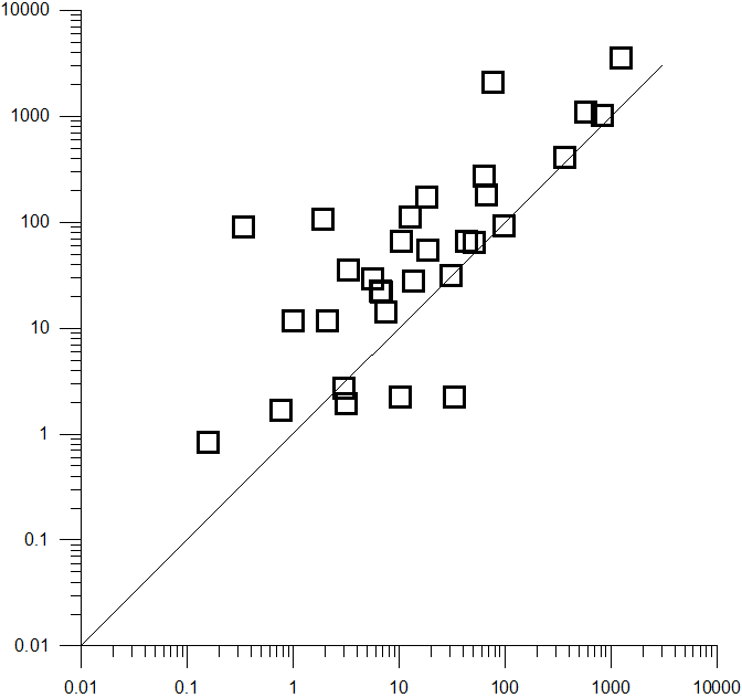
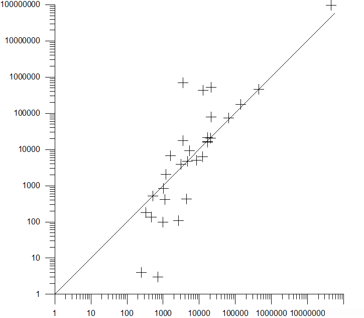
(a)	(b)
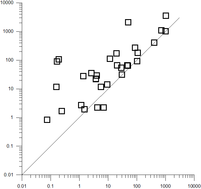
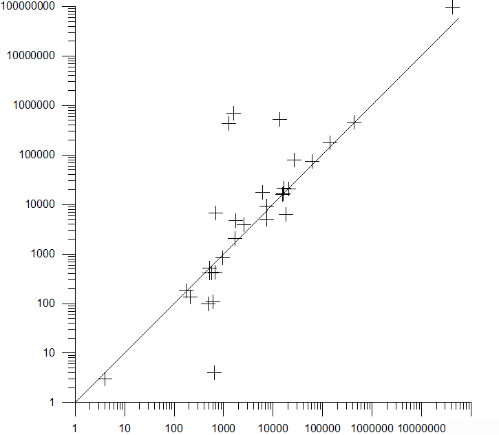
(c)	(d)
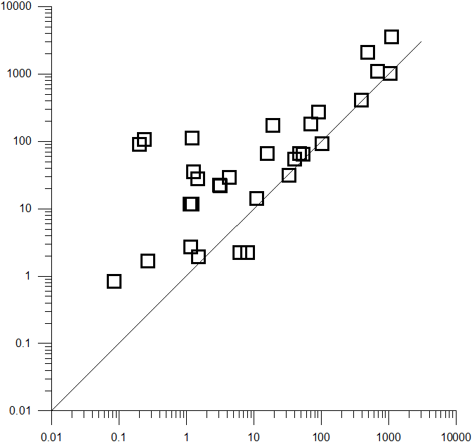
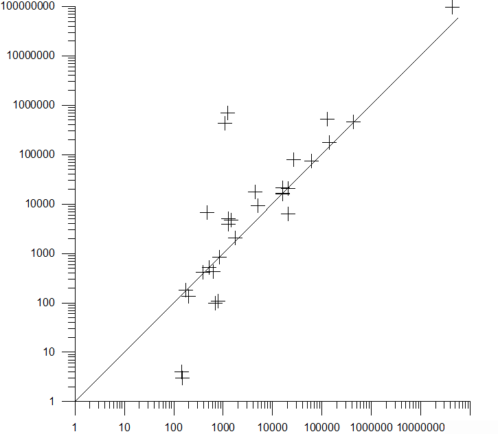
(e)	(f)

Figure 1: A summary view of run times (left figures) and nodes visited (right figures), for $dom/wdeg$ and $impact$ heuristics (figures (a),(b)), “alldell” and $impact$ heuristics (figures (c),(d)), “fully assigned” and $impact$ heuristics (figures (e),(f)).

5 Conflict-driven revision ordering heuristics

Having demonstrated that conflict-driven heuristics such as dom/wdeg are the dominant modern variable ordering heuristics, we turn our attention to the use of failures discovered during search in a different context. To be precise, we investigate their use in devising heuristics for the ordering of the (G)AC revision list.

It is well known that the order in which the elements of the revision list are processed affects the overall cost of the search [38, 7, 34]. This is true for solvers that implement variable or constraint based propagation as well as for propagator oriented solvers like Ilog Solver and Geocode. In general, revision ordering and variable ordering heuristics have different tasks to perform when used by a search algorithm like MAC. Prior to the emergence of conflict-driven heuristics there was no way to achieve an interaction with each other, i.e. the order in which the revision list was organized during the application of AC could not affect the decision of which variable to select next (and vice versa). The contribution of revision ordering heuristics to the solver’s efficiency was limited to the reduction of list operations and constraint checks.

In this section we first show that the ordering of the revision list can affect the decisions taken by a conflict-driven DVO heuristic. That is, different orderings can lead to different parts of the search space being explored. Based on this observation, we then present a set of new revision ordering heuristics that use constraint weights, which can not only reduce the numbers of constraints checks and list operations, but also cut down the size of the explored search tree. Finally, we demonstrate that some conflict-driven DVO heuristics, e.g. “alldel” and “fully assigned”, are less amenable to changes in the revision list ordering than others (e.g. dom/wdeg).

First of all, to illustrate the interaction between a conflict-driven variable ordering heuristic and revision list orderings, we give the following example.

Example 1

Assume that we want to solve a CSP $(X,D,C)$, where X contains n variables {$x_{1},x_{2},...,x_{n}$}, using a conflict-driven variable ordering heuristic (e.g. dom/wdeg), and that at some point during search and propagation the variables pending for revision are $x_{1}$ and $x_{5}$. Also assume that two of the constraints in the problem are $x_{1}>x_{2}$ and $x_{5}>x_{6}$, and that the domains of $x_{1},x_{2},x_{5},x_{6}$ are as follows: $D(x_{1})=D(x_{5})=\{0,1\}$, $D(x_{2})=D(x_{6})=\{2,3\}$. Given these constraints and domains, the revision of $x_{1}$ against $x_{2}$ would result in the DWO of $x_{1}$, and the revision of $x_{5}$ against $x_{6}$ would result in the DWO of $x_{5}$. Independent of which variable is selected to be revised first (i.e. either $x_{1}$ or $x_{5}$), a DWO will be detected and the solver will reject the current variable assignment. However, depending on the order of revisions, the dom/wdeg heuristic will increase the weight of a different constraint. To be precise, if a revision ordering heuristic $R_{1}$ selects to revise $x_{1}$ first then the DWO of $D(x_{1})$ will be detected and the weight of constraint $c_{12}$ will be increased by 1. If some other revision ordering heuristic $R_{2}$ selects $x_{5}$ first then the DWO of $D(x_{5})$ will be detected, but this time the weight of constraint $c_{56}$ will be increased by 1. Since increases in constraint weights affect the subsequent choices of the variable ordering heuristic, $R_{1}$ and $R_{2}$ can lead to different future decisions for variable instantiation. Thus, $R_{1}$ and $R_{2}$ may guide search to different parts of the search space.

From the above example it becomes clear that the revision ordering can have an important impact on the performance of conflict-driven heuristics like dom/wdeg. One might argue that a way to overcome this is to continue propagation after the first DWO is detected, try to identify all possible DWOs and increase the weights of all constraints involved in failures. The problem with this approach is threefold: First, it may increase the cost of constraint propagation significantly, second it requires modifications in the way all solvers implement constraint propagation (i.e. stopping after a failure is detected), and third, experiments we have run showed that the possibility of more than one DWO occurring is typically very low. As we will discuss in Section 5.5, some variants of dom/wdeg are less amenable to different revision orderings, i.e. their performance do not depend on the ordering as much, without having to implement this potentially complex approach.

In the following we first review three standard implementations of revision lists for AC, i.e. the arc-oriented, variable-oriented, and constraint-oriented variants. Then, we summarize the major revision ordering heuristics that have been proposed so far in the literature, before describing the new efficient revision ordering heuristics we propose.

5.1 AC variants

The numerous AC algorithms that have been proposed can be classified into coarse grained and fine grained. Typically, coarse grained algorithms like AC-3 [25] and its extensions (e.g. AC2001/3.1 [6] and AC-$3_{d}$ [16]) apply successive revisions of arcs, variables, or constraints. On the other hand, fine grained algorithms like AC-4 [28] and AC-7 [4] use various data structures to apply successive revisions of variable-value-constraint triplets. Here we are concerned with coarse grained algorithms, and specifically AC-3. There are two reasons for this. First, although AC-3 does not have an optimal worst-case time complexity, as the fine grained algorithms do, it is competitive and often better in practice and has the additional advantage of being easy to implement. Second, many constraint solvers that can handle constraints of any arity follow the philosophy of coarse grained AC algorithms in their implementation of constraint propagation. That is, they apply successive revisions of variables or constraints. Hence, the revision ordering heuristics we describe below can be easily incorporated into most of the existing solvers.

As mentioned, the AC-3 algorithm can be implemented using a variety of propagation schemes. We recall here the three variants, following the presentation of [7], which respectively correspond to algorithms with an arc-oriented, variable-oriented or constraint-oriented propagation scheme.

The first one (arc-oriented propagation) is the most commonly presented and used because of its simple and natural structure. Algorithm 1 depicts the main procedure. As explained, an arc is a pair ($c_{ij},x_{j}$) which corresponds to a directed constraint. Hence, for each binary constraint $c_{ij}$ involving variables $x_{i}$ and $x_{j}$ there are two arcs, ($c_{ij},x_{j}$) and ($c_{ij},x_{i}$). Initially, the algorithm inserts all arcs in the revision list Q. Then, each arc ($c_{ij},x_{j}$) is removed from the list and revised in turn. If any value in $D(x_{j})$ is removed when revising ($c_{ij},x_{j}$), all arcs pointing to $x_{j}$ (i.e. having $x_{i}$ as second element in the pair), except ($c_{ij},x_{i}$), will be inserted in Q (if not already there) to be revised. Algorithm 2 depicts function REVISE($c_{ij},x_{j}$) which seeks supports for the values of $x_{j}$ in $D(x_{i})$. It removes those values in $D(x_{j})$ that do not have any support in $D(x_{i})$. The algorithm terminates when the list Q becomes empty.

Algorithm 1 arc-oriented AC3

1:  $Q\leftarrow${($c_{ij}$, $x_{j}$) $|$ $c_{ij}\in C$ and $x_{j}\in vars(c_{ij})$}

2:  while $Q\neq\emptyset$ do

3:     select and delete an arc ($c_{ij}$, $x_{j}$) from Q

4:     if REVISE($c_{ij}$, $x_{j}$) then

5:        Q $\leftarrow$ Q $\cup$ {($c_{kj}$, $x_{k}$) $|$ $c_{kj}\in C,k\neq i$}

6:     end if

7:  end while

Algorithm 2 $\mbox{\sc revise}(\emph{$c_{ij}$, $x_{i}$})$

1:  DELETE $\leftarrow$ false

2:  for each a $\in$ $D(x_{i})$ do

3:     if $\nexists$ b $\in$ $D(x_{j})$ such that (a, b) satisfies $c_{ij}$ then

4:        delete a from $D(x_{i})$

5:        DELETE $\leftarrow$ true

6:     end if

7:  end for

8:  return  DELETE

Algorithm 3 variable-oriented AC3

1:  Q $\leftarrow$ {$x_{i}$ $|$ $x_{i}\in X$}

2:  $\forall$ $c_{ij}\in C,\forall x_{i}\in$ vars($c_{ij}$), ctr($c_{ij},x_{i}$) $\leftarrow$ 1

3:  while Q $\neq$ $\emptyset$ do

4:     get $x_{i}$ from Q

5:     for each $c_{ij}$ $|$ $x_{i}\in$ vars($c_{ij}$) do

6:        if ctr($c_{ij},x_{i}$) = 0 then continue

7:        for each $x_{j}\in vars(c_{ij})$ do

8:           if NEEDS-NOT-BE-REVISED($c_{ij},x_{j}$) then continue

9:           nbRemovals $\leftarrow$ REVISE($c_{ij},x_{j}$)

10:           if nbRemovals $>$ 0 then

11:              if dom($x_{j}$) = $\emptyset$ then return false

12:              Q $\leftarrow$ Q $\cup$ {$x_{j}$}

13:              for each $c_{jk}$ $|$ $c_{jk}\neq c_{ij}\wedge x_{j}\in$ vars($c_{jk}$) do

14:                 ctr($c_{jk},x_{j}$) $\leftarrow$ ctr($c_{jk},x_{j}$) + nbRemovals

15:              end for

16:           end if

17:        end for

18:        for each $x_{j}\in$ vars($c_{ij}$) do ctr($c_{ij},x_{j}$) $\leftarrow$ 0

19:     end for

20:  end while

21:  return  true

Algorithm 4 needs-not-be-revised($c_{ij},x_{i}$)

1:  return (ctr($c_{ij},x_{i}$) $>$ 0 and $\nexists x_{j}\in$ vars($c_{ij}$) $|$ $x_{j}\neq x_{i}$ $\wedge$ ctr($c_{ij},x_{j}$) $>$ 0)

Algorithm 5 constraint-oriented AC3

1:  Q $\leftarrow$ {$c_{ij}$ $|$ $c_{ij}\in C$}

2:  $\forall$ $c_{ij}\in C,\forall x_{i}\in$ vars($c_{ij}$), ctr($c_{ij},x_{i}$) $\leftarrow$ 1

3:  while Q $\neq$ $\emptyset$ do

4:     get $c_{ij}$ from Q

5:     for each $x_{j}\in vars(c_{ij})$ do

6:        if NEEDS-NOT-BE-REVISED($c_{ij},x_{j}$) then continue

7:        nbRemovals $\leftarrow$ REVISE($c_{ij},x_{j}$)

8:        if nbRemovals $>$ 0 then

9:           if dom($x_{j}$) = $\emptyset$ then return false

10:           for each $c_{jk}$ $|$ $c_{jk}\neq c_{ij}\wedge x_{j}\in$ vars($c_{jk}$) do

11:              Q $\leftarrow$ Q $\cup$ {$x_{j}$}

12:              ctr($c_{jk},x_{j}$) $\leftarrow$ ctr($c_{jk},x_{j}$) + nbRemovals

13:           end for

14:        end if

15:     end for

16:     for each $x_{j}\in$ vars($c_{ij}$) do ctr($c_{ij},x_{j}$) $\leftarrow$ 0

17:  end while

18:  return  true

The variable-oriented propagation scheme was proposed by McGregor [27] and later studied in [12]. Instead of keeping arcs in the revision list, this variant of AC-3 keeps variables. The main procedure is depicted in Algorithm 3. Initially, all variables are inserted in the revision list Q. Then each variable $x_{i}$ is removed from the list and each constraint involving $x_{i}$ is processed. For each such constraint $c_{ij}$ we revise the arc ($x_{j}$,$x_{i}$). If the revision removes some values from the domain of $x_{j}$, then variable $x_{j}$ is inserted in Q (if not already there).

Function NEEDS-NOT-BE-REVISED given in Algorithm 4, is used to determine relevant revisions. This is done by associating a counter $ctr$($c_{ij}$,$x_{i}$) with any arc ($x_{i}$,$x_{j}$). The value of the counter denotes the number of removed values in the domain of variable $x_{i}$ since the last revision involving constraint $c_{ij}$. If $x_{i}$ is the only variable in $vars(c_{ij})$ that has a counter value greater than zero, then we only need to revise arc ($x_{j}$,$x_{i}$). Otherwise, both arcs are revised.

The constraint-oriented propagation scheme is depicted in Algorithm 5. This algorithm is an analogue to Algorithm 3. Initially, all constraints are inserted in the revision list Q. Then each constraint $c_{ij}$ is removed from the list and each variable $x_{j}\in vars(c_{ij})$ is selected and revised. If the revision of the selected arc ($c_{ij}$, $x_{j}$) is fruitful, then the reinsertion of the constraint $c_{ij}$ in the list is needed. As in the variable-oriented scheme, the same counters are also used here to avoid useless revisions.

5.2 Overview of revision ordering heuristics

Revision ordering heuristics is a topic that has received considerable attention in the literature. The first systematic study on this topic was carried out by Wallace and Freuder, who proposed a number of different heuristics that can be used with the arc-oriented variant of AC-3 [38]. These heuristics, which are defined for binary constraints, are based on three major features of CSPs: (i) the number of acceptable pairs in each constraint (the constraint size or satisfiability), (ii) the number of values in each domain and (iii) the number of binary constraints that each variable participates in (the degree of the variable). Based on these features, they proposed three revision ordering heuristics: (i) ordering the list of arcs by increasing relative satisfiability (sat up), (ii) ordering by increasing size of the domain of the variables (dom j up) and (iii) ordering by descending degree of each variable (deg down).

The heuristic sat up counts the number of acceptable pairs of values in each constraint (i.e the number of tuples in the Cartesian product built from the current domains of the variables involved in the constraint) and puts constraints in the list in ascending order of this count. Although this heuristic reduces the list additions and constraint checks, it does not speed up the search process. When a value is deleted from the domain of a variable, the counter that keeps the number of acceptable arcs has to be updated. This process is usually time consuming because the algorithm has to identify the constraints in which the specific variable participates and to recalculate the counters with acceptable value pairs. Also an additional overhead is needed to reorder the list.

The heuristic dom j up counts the number of remaining values in each variable’s current domain during search. Variables are inserted in the list by increasing size of their domains. This heuristic reduces significantly list additions and constraint checks and is the most efficient heuristic among those proposed in [38].

The deg down heuristic counts the current degree of each variable. The initial degree of a variable $x_{i}$ is the number of variables that share a constraint with $x_{i}$. During search, the current degree of $x_{i}$ is the number of unassigned variables that share a constraint with $x_{i}$. The deg down heuristic sorts variables in the list by decreasing size of their current degree. As noticed in [38] and confirmed in [7], the (deg down) heuristic does not offer any improvement.

Gent et al. [19] proposed another heuristic called $k_{ac}$. This heuristic is based on the number of acceptable pairs of values in each constraint and tries to minimize the constrainedness of the resulting subproblem. Experiments have shown that $k_{ac}$ is time expensive but it performs less constraint checks when compared to sat up and dom j up.

Boussemart et al. [7] performed an empirical investigation of the heuristics of [38] with respect to the different variants (arc, variable and constraint) of AC-3. In addition, they introduced some new heuristics. Concerning the arc-oriented AC-3 variant, they have examined the dom j up as a stand alone heuristic (called $dom^{v}$) or together with deg down which is used in order to break ties (called $ddeg\circ dom^{v}$). Moreover, they proposed the ratio sat up/dom j up (called $dom^{c}/dom^{v}$) as a new heuristic. Regarding the variable-oriented variant, they adopted the $dom^{v}$ and $ddeg$ heuristics from [38] and proposed a new one called $rem^{v}$. This heuristic corresponds to the greatest proportion of removed values in a variable’s domain. For the constraint-oriented variant they used $dom^{c}$ (the smallest current domain size) and $rem^{c}$ (the greatest proportion of removed values in a variable’s domain). Experimental results showed that the variable-oriented AC-3 implementation with the $dom^{v}$ revision ordering heuristic (simply denoted $dom$ hereafter) is the most efficient alternative.

5.3 Revision ordering heuristics based on constraint weights

The heuristics described in the previous subsection, and especially $dom$, improve the performance of AC-3 (and MAC) when compared to the classical queue or stack implementation of the revision list. This improvement in performance is due to the reduction in list additions and constraint checks. A key principle that can have a positive effect on the performance of the AC algorithms is the “ASAP principle” by Wallace and Freuder [38] which urges to “remove domain values as soon as possible”. Considering revision ordering heuristics this principle can be translated as follows: When AC is applied during search (within an algorithm such as MAC), to reach as early as possible a failure (DWO), order the revision list by putting first the arc or variable which will guide you to early value deletions and thus, most likely, earlier to a DWO.

To apply the “ASAP principle” in revision ordering heuristics, we must use some metric to compute which arc (or variable) in the AC revision list is the most likely to cause failure. Until now, constraint weights have only been used for variable selection. In the next paragraphs we describe a number of new revision ordering heuristics for all three AC-3 variants. These heuristics use information about constraint weights as a metric to order the AC revision list and they can be used efficiently in conjunction with conflict-driven variable ordering heuristics to boost search.

The main idea behind these new heuristics is to handle as early as possible potential DWO-revisions by appropriately ordering the arcs, variables, or constraints in the revision list. In this way the revision process of AC will be terminated earlier and thus constraint checks can be reduced significantly. Moreover, with such a design we may be able to avoid many redundant revisions. As will become clear, all of the proposed heuristics are lightweight (i.e. cheap to compute) assuming that the weights of constraints are updated during search.

Arc-oriented heuristics are tailored for the arc-oriented variant where the list of revisions Q stores arcs of the form ($c_{ij}$,$x_{i}$). Since an arc consists of a constraint $c_{ij}$ and a variable $x_{i}$, we can use information about the weight of the constraint, or the weight of the variable, or both, to guide the heuristic selection. These ideas are the basis of the proposed heuristics described below. For each heuristic we specify the arc that it selects. The names of the heuristics are preceded by an “a” to denote that they are tailored for arc-oriented propagation.

• $a\_wcon$: selects the arc ($c_{ij}$,$x_{i}$) such that $c_{ij}$ has the highest weight wcon among all constraints appearing in an arc in Q.

• $a\_wdeg$: selects the arc ($c_{ij}$,$x_{i}$) such that $x_{i}$ has the highest weighted degree wdeg among all variables appearing in an arc in Q.

• $a\_dom/wdeg$: selects the arc ($c_{ij}$,$x_{i}$) such that $x_{i}$ has the smallest ratio between current domain size and weighted degree among all variables appearing in an arc in Q.

• $a\_dom/wcon$: selects the arc ($c_{ij}$,$x_{i}$) having the smallest ratio between the current domain size of $x_{i}$ and the weight of $c_{ij}$ among all arcs in Q.

The call to one of the proposed arc-oriented heuristics can be attached to line 3 of Algorithm 1. Note that heuristics $a\_dom/wdeg$ and $a\_dom/wcon$ favor variables with small domain size hoping that the deletion of their few remaining values will lead to a DWO. To strictly follow the “ASAP principle” which calls for early value deletions we intend to evaluate the following heuristics in the future:

• $a\_dom/wdeg\_inverse$: selects the arc ($c_{ij}$,$x_{i}$) such that $x_{j}$ has the smallest ratio between current domain size and weighted degree among all variables appearing in an arc in Q.

• $a\_dom/wcon\_inverse$: selects the arc ($c_{ij}$,$x_{i}$) having the smallest ratio between the current domain size of $x_{j}$ and the weight of $c_{ij}$ among all arcs in Q.

Heuristics $a\_dom/wdeg\_inverse$ and $a\_dom/wcon\_inverse$ favor revising arcs ($c_{ij}$,$x_{i}$) such that $x_{j}$, i.e. the other variable in constraint $c_{ij}$, has small domain size. This is because in such cases it is more likely that some values in $D(x_{i})$ will not be supported in $D(x_{j})$, and hence will be deleted.

Variable-oriented heuristics are tailored for the variable-oriented variant of AC-3 where the list of revisions Q stores variables. For each of the heuristics given below we specify the variable that it selects. The names of the heuristics are preceded by an “v” to denote that they are tailored for variable-oriented propagation.

• $v\_wdeg$: selects the variable having the highest weighted degree wdeg among all variables in Q.

• $v\_dom/wdeg$: selects the variable having the smallest ratio between current domain size and wdeg among all variables in Q.

The call to one of the proposed variable-oriented heuristics can be attached to line 4 of Algorithm 3. After selecting a variable, the algorithm revises, in some order, the constraints in which the selected variable participates (line 5). Our heuristics process these constraints in descending order according to their corresponding weight.

Finally, the constraint-oriented heuristic $c\_wcon$ selects a constraint $c_{ij}$ from the AC revision list having the highest weight among all constraints in Q. The call to this heuristic can be attached to line 4 of Algorithm 5. One can devise more complex constraint-oriented heuristics by aggregating the weighted degrees of the variables involved in a constraint. However, we have not yet implemented such heuristics.

5.4 Experiments with revision ordering heuristics

In this section we experimentally investigate the behavior of the new revision ordering heuristics proposed above on several classes of real world, academic and random problems. We only include results for the two most significant arc consistency variants: arc and variable oriented. We have excluded the constraint-oriented variant since this is not as competitive as the other two [7].

We compare our heuristics with $dom$, the most efficient previously proposed revision ordering heuristic. We also include results from the standard fifo implementation of the revision list which always selects the oldest element in the list (i.e. the list is implemented as a queue). In our tests we have used the following measures of performance: cpu time in seconds (t), number of visited nodes (n), number of constraint checks (c) and the number of times (r) a revision ordering heuristic has to select an element in the propagation list $Q$.

Tables 9 and 10 show results from some real-world RLFAP instances. In the arc-oriented implementation of AC-3 (Table 9), heuristics $a\_wcon$, mainly, and $a\_dom/wcon$, to a less extent, decrease the number of constraint checks and list revisions compared to $dom$. However, the decrease is not substantial and is rarely leads into a decrease in cpu times. The notable speed-up observed for problem s11-f6 is mainly due to the reduction in the number of visited nodes offered by the two new heuristics. $a\_wdeg$ and $a\_dom/wdeg$ are less competitive, indicating that information about the variables involved in arcs is less important compared to information about constraints.

The variable-oriented implementation (Table 10) is clearly more efficient than the arc-oriented one. This confirms the results of [7]. Concerning this implementation, heuristic $v\_dom/wdeg$ in most cases is better than $dom$ and $queue$ in all the measured quantities (number of visited nodes, constraint checks and list revisions). Importantly, these savings are reflected on notable cpu time gains making the variable-oriented heuristic $v\_dom/wdeg$ the overall winner. Results also show that as the instances becomes harder, the efficiency of $v\_dom/wdeg$ compared to $dom$ increases. The variable-oriented $v\_wdeg$ heuristic in most cases is better than $dom$ but is clearly less efficient than $v\_dom/wdeg$.

Table 9: Cpu times (t), constraint checks (c), number of list revisions (r) and nodes (n) from frequency allocation problems (hard instances) using arc oriented propagation. The s prefix stands for scen instances. Best cpu time is in bold.

		ARC ORIENTED
Inst.		$queue$	$dom$	$a\_wcon$	$a\_wdeg$	$a\_dom/wdeg$	$a\_dom/wcon$
s11-f9	t	18,8	12,8	14,6	14,8	19	14,2
	c	25,03M	19,3M	13,2M	20,8M	21M	16,8M
	r	1,1M	910060	529228	1,04M	1,01M	737803
	n	1202	1153	1155	1145	1148	1159
s11-f8	t	37,5	20,3	22,5	21,9	28,5	23,5
	c	46,5M	29,3M	19,1M	30,1M	32,9M	27,5M
	r	1,95M	1,3M	748050	1,52M	1,43M	1,11M
	n	1982	1830	1843	1876	1832	1928
s11-f7	t	257,5	146,5	170	265,2	205,8	326,2
	c	268,4M	159,4M	128,5M	281,4M	205,1M	300M
	r	13,3M	10,2M	6,1M	17,7M	12,1M	15M
	n	17643	14734	15938	20617	15318	29845
s11-f6	t	568,5	465,2	309,4	540,4	834,9	396,4
	c	482,3M	468,2M	230,8M	517,2M	745,4M	362,7M
	r	27,5M	29,7M	10,4M	34,9M	49,5M	16,6M
	n	46671	50021	29057	49201	68217	35860
s11-f5	t	2821	2307	3064	3234	2898	2291
	c	2,492G	2,139G	2,097G	2,928G	2,596G	1,965G
	r	137,8M	157M	116,5M	215,7M	172,2M	103,3M
	n	212012	217407	287017	258261	185991	187363
s11-f4	t	11216	7774	8256	10386	12520	10473
	c	9,938G	7,054G	5,298G	9,020G	10,711G	8,598G
	r	533,4M	523,1M	311,7M	681,2M	738,1M	464,7M
	n	753592	709196	762477	832892	850446	786924

Table 10: Cpu times (t), constraint checks (c), number of list revisions (r) and nodes (n) from frequency allocation problems (hard instances) using variable oriented propagation. The s prefix stands for scen instances. Best cpu time is in bold.

		VARIABLE ORIENTED
Inst.		$queue$	$dom$	$v\_wdeg$	$v\_dom/wdeg$
s11-f9	t	14,3	10,2	10,9	9,9
	c	22,6M	11,4M	12,9M	11M
	r	28978	17177	20161	17048
	n	1413	1117	1145	1137
s11-f8	t	21,2	17,3	18,5	16,7
	c	42,1M	17,2M	20,4M	16,8M
	r	48568	24885	28807	24819
	n	2112	1842	1830	1841
s11-f7	t	133,7	158,1	154,5	108,2
	c	193,3M	116,9M	157,6M	82,7M
	r	313568	223094	263306	156160
	n	12777	18773	14570	13181
s11-f6	t	391,4	391	434,4	269,5
	c	306,2M	263,2M	413,6M	192,6M
	r	426469	509474	673935	340583
	n	34714	46713	41609	31538
s11-f5	t	2473	3255	2019	1733
	c	2,073G	2,115G	1,502G	1,157G
	r	3,63M	4,52M	2,97M	2,2M
	n	223965	397590	190496	199854
s11-f4	t	13969	11859	9490	6669
	c	12,059G	7,512G	6,915G	4,322G
	r	20,3M	15,9M	14M	8,9M
	n	1,148M	1,354M	939094	716427

In Table 11 we present results from structured instances belonging to benchmark classes langford and driver. As the variable-oriented AC-3 variant is more efficient than the arc-oriented one, we only present results from the former. Results show that on easy problems all heuristics except $queue$ are quite competitive. But as the difficulty of the problem increases, the improvement offered by the $v\_dom/wdeg$ revision heuristic becomes clear. On instance driverlogw-09 we can see the effect that weight based revision ordering heuristics can have on search. $v\_dom/wdeg$ cuts down the number of node visits by more than 5 times resulting in a similar speed-up. It is interesting that $v\_dom/wdeg$ is considerably more efficient than $v\_wdeg$ and $dom$, indicating that information about domain size or weighted degree alone is not sufficient to efficiently order the revision list.

Table 11: Cpu times (t), constraint checks (c), number of list revisions (r) and nodes (n) from structured problems using variable oriented propagation. Best cpu time is in bold.

Instance		$queue$	$dom$	$v\_wdeg$	$v\_dom/wdeg$
langford-2-9	t	56,5	46,9	60,3	46,2
	c	99,6M	81,7M	99,9M	81,5M
	r	633113	533656	741596	533261
	n	48533	40228	49114	40363
langford-2-10	t	489,8	430,6	418,9	340,1
	c	336,1M	283,7M	275,2M	197,9M
	r	5,3M	4,5M	4M	2,9M
	n	337772	280600	260343	208651
langford-3-11	t	695,8	648,5	843,5	513,5
	c	408,6M	352,7M	468,8M	256,7M
	r	2,3M	1,9M	2,9M	1,6M
	n	99508	68042	103863	65958
langford-4-10	t	81,4	57,7	99,4	41,2
	c	52,3M	33,2M	59,6M	21,7M
	r	150493	99646	194952	75889
	n	3852	2973	5759	2661
driverlogw-08c	t	19,4	14,7	14,4	14,6
	c	20,8M	8,6M	10,9M	9M
	r	86809	39063	40256	38748
	n	3151	3040	1960	2660
driverlogw-09	t	174,6	411	346,3	70,1
	c	151,5M	251,5M	203,6M	39,5M
	r	521358	1,05M	583686	139962
	n	21220	41039	31548	7457

Finally, in Table 12 we present results from random and quasi-random problems. In the geo50-20-d4-75-2 , which is a quasi-random instance we can see that the proposed heuristics ($v\_wdeg$ and $v\_dom/wdeg$) are one order of magnitude faster than $dom$. This suggest that the small presence of structure is this problem results in behavior similar to the behavior observed in the structured instances of Table 11.

On the rest of the instances, which are purely random, there is a large variance in the results. All heuristics seems to lack robustness and there is no clear winner. The constraint weight based heuristics can be faster than $dom$ (instance frb30-15-1), but they can also be significantly slower (frb30-15-2). In all cases, the large run time differences in favor of one or another heuristic are caused by corresponding differences in the size of the explored search tree, as node visits clearly demonstrate.

A plausible explanation for the diversity in the performance of the heuristics on pure random problems as opposed to structured ones is the following. When dealing with structured problems, and assuming we use the variable-oriented variant of AC-3, a weighted based heuristic like $v\_dom/wdeg$ will give priority for revision to variables that are involved in hard subproblems and hence will carry out DWO-revisions faster. This will in turn increase the weights of constraints that are involved in such hard subproblems and thus search will focus on the most important parts of the search space. Pure random instances that lack structure do not in general consist of hard local subproblems. Thus, different decisions on which variables to revise first can lead to different DWO-revisions being discovered, which in turn can guide search tree to different parts of the search space with unpredictable results. Note that for structured problems only very few possible DWO-revisions are present in the revision list at each point in time, while for random ones there can be a large number of such revisions.

Table 12: Cpu times (t), constraint checks (c), number of list revisions (r) and nodes (n) from random problems using variable oriented propagation. Best cpu time is in bold.

Instance		$queue$	$dom$	$v\_wdeg$	$v\_dom/wdeg$
frb30-15-1	t	22,3	20,9	29,3	14,1
	c	16,5M	11,1M	16,4M	7,5M
	r	105626	70924	102724	46727
	n	3863	3858	4138	2499
frb30-15-2	t	84,9	29,7	118,9	95
	c	45,7M	21,8M	90M	68,9M
	r	311040	149119	624360	472124
	n	15457	7935	25148	24467
frb35-17-1	t	125,8	193,7	118	250,9
	c	93,9M	144M	89,7M	180,9M
	r	533694	836462	514258	1,03M
	n	18587	40698	19167	50611
rand-2-30-15	t	1240	74,4	98	108,1
	c	114,5M	53M	72,5M	78,1M
	r	922251	443792	602582	642665
	n	28725	19846	20192	28766
geo50-20-d4-75-2	t	226,1	401,8	34,8	39,5
	c	191,8M	310,3M	28,2M	28,8M
	r	778758	1,3M	117241	124163
	n	20069	60182	3735	5484

5.5 Dependency of conflict-driven heuristics on the revision ordering

As we showed in the previous section, dom/wdeg is strongly dependent on the order in which the revision list is constructed and updated during constraint propagation. Looking at the results in Tables 9 – 12, we can see that there are cases where the differences in cpu performance between $dom$ and $v\_dom/wdeg$ can be up to 5 times. Hence, when dom/wdeg is used as DVO heuristic, we must carefully select a good revision ordering using for example one of the heuristics we have proposed in Section 5.3. In contrast, the conflict-driven DVO heuristics “alldel” and “fully assigned” are not as amenable to the selection of revision ordering. To better illustrate this statement, let us consider the following example.

Example 2

Assume that we want to solve a CSP $(X,D,C)$ with $X$: {$x_{1}$, $x_{2}$, $x_{3}$, $x_{4}$}, by using two different revision ordering heuristics $R_{1}$ (lexicographic ordering) and $R_{2}$ (reverse lexicographic ordering). For the revision of each $x_{i}$ $\in$ $X$, we assume that the following hypotheses are true: a) The revision of $x_{1}$ is fruitful and it causes the addition of the variable $x_{3}$ in the revision list. b) The revision of $x_{2}$ is fruitful and it causes the addition of the variable $x_{4}$ in the revision list. c) The revision of $x_{4}$ is fruitful and it causes the addition of the variable $x_{3}$. We also assume the a DWO can only occur either d) in $x_{4}$ after a sequential revision of $x_{2}$ and $x_{3}$ or e) in $x_{3}$ after a sequential revision of $x_{4}$ and $x_{1}$. Finally, assume that at some point during search only the variables $x_{1}$ and $x_{2}$ have remained in the AC revision list $Q$, but with different orderings for $R_{1}$ and $R_{2}$. That is, $Q_{R_{1}}$:{$x_{1}$,$x_{2}$}, $Q_{R_{2}}$:{$x_{2}$,$x_{1}$}. Following all these assumptions (which can exist commonly in any real world CSP), lets now trace the behavior of both $R_{1}$ and $R_{2}$ during problem solving. Considering the $Q_{R_{1}}$ list, the revision of $x_{1}$ is fruitful and adds $x_{3}$ in the list (due to hypothesis $a$). Now the revision list changes to $Q_{R_{1}}$:{$x_{2}$,$x_{3}$}. The sequential revision of $x_{2}$ and $x_{3}$ leads to the DWO of $x_{4}$ (due to hypotheses $b$ and $d$). Considering the $Q_{R_{2}}$ list, the revision of $x_{2}$ is fruitful and adds $x_{4}$ in the list (due to hypothesis $b$). Now the revision list changes to $Q_{R_{2}}$:{$x_{4}$,$x_{1}$}. The sequential revision of $x_{4}$ and $x_{1}$ leads to the DWO of $x_{3}$. (due to hypotheses $c$ and $e$).

From the above example it is clear that although only one DWO is identified in the revision list, both $x_{1}$ and $x_{2}$ can be responsible for this. In $R_{1}$ where $x_{1}$ is the DWO variable, we can say that $x_{2}$ is also a “potential” DWO variable i.e. it would be a DWO variable, if the $R_{2}$ revision ordering was used. Although the dom/wdeg heuristic ignores all the “potential” DWO variables, the other two DVO heuristics,“alldel” and “fully assigned”, take into account their contribution. The former heuristic increases the weights for every constraint that causes a value deletion, and thus succeeds to increase the weights of the constraints related to the “potential” DWO variables. The latter heuristic increases the weights of constraints that participate in fruitful revisions (only for revision lists that lead to a DWO), and thus is able to frequently identify “potential” DWO variables.

To experimentally verify the strong dependance of $dom/wdeg$ heuristic on the revision ordering and the ability of the “alldel” and “fully assigned” heuristics to be less dependent, we have computed the variance in the number of node visits for the three conflict-driven heuristics on some selected instances.

The variance is a measure of how spread out a distribution of a variable’s values is. A variable’s spread is the degree to which the values of the variable differ from each other. If all values of the variable were about equal, the variable would have very little spread. In other words, it is a measure of variability. In our case the measured variable $x$ is the number of visited nodes for the conflict-driven heuristics. For each conflict-driven heuristic the $x$ variable can take $N$=3 values. That is, the number of visited nodes when any one of the 3 main revision ordering heuristics ($queue$, $dom$, $v\_dom/wdeg$) is used.

The variance is calculated by taking the arithmetic mean of the squared differences between each value and the mean value, using the following equation:

$$VARIANCE=\frac{\sum(x-\bar{x})^{2}}{N}$$ (4)

where $x$ is the number of node visits when a specific revision ordering heuristic is used and $\bar{x}$ is the mean number of visited nodes of the $N$=3 main revision ordering heuristics ($queue$, $dom$, $v\_dom/wdeg$).

The smaller the variance of a conflict-driven heuristic, the less the dependance from the selected revision ordering heuristic. Results from these experiments are depicted in Table 13. As we can see, in almost all cases the $dom/wdeg$ heuristic displays the highest variance, while the other two conflict-driven heuristics in most cases have smaller values. This suggests that indeed the “alldel” and “fully assigned” heuristics are less amenable to changes in the revision ordering than dom/wdeg and therefore can be more robust.

Table 13: The computed variances for the three conflict-driven heuristics. Best values is in bold.

Instance	$dom/wdeg$	$alldel$	$fully$ $assigned$
scen-11	96732	7432	67
scen-11-f8	6893	2127	701
scen-11-f7	3974589	6384509	1454538
jnh01	6123	80	41280
jnh17	1316	52	91
jnh201	4238	12	7
jnh301	66738	19783	91
langford-2-10	7564932	4547893	10923451
driverlogw-08c	291287	8465	912
driverlogw-09	71643951	19821345	13189345
will199GPIA-5	1139	0	3717
will199GPIA-6	5313746	860138	614930

Finally, it would be interesting to apply similar ideas as the ones presented in Section 5 to propagator-heavy solvers. Constraint propagation in such solvers is not handled by a revision list of variables or constraints, but they do use heuristics to choose the order in which propagators will be applied [34]. Hence taking exploiting information such as constraint weights might be beneficial.

6 Conclusions and future work

In this paper we experimentally evaluated the most recent and powerful variable ordering heuristics, and new variants of them, over a wide range of academic, random and real world problems. These heuristics can be divided in two main categories: heuristics that exploit information about failures gathered throughout search and recorded in the form of constraint weights and heuristics that measure the importance/impact of variable assignments for reducing the search space. Results demonstrate that heuristics based on failures have much better cpu performance. Although impact based heuristics are in general slow, there are some cases where they perform a smarter exploration of the search tree resulting in fewer node visits. Among the tested conflict-driven heuristics, dom/wdeg seems to be the faster followed closely by its variants “alldel” and “fully assigned”.

We also showed how information about failures can be exploited to design efficient revision ordering heuristics for algorithms that maintain (G)AC using coarse grained arc consistency algorithms. The proposed heuristics order the revision list by trying to carry out possible DWO-revisions as soon as possible. Importantly, these heuristics can not only reduce the numbers of constraint checks and list operations but they can also have a significant effect on search. Among the revision ordering heuristic we experimented with, the one with best performance was $v\_dom/wdeg$ in the variable-oriented implementation of arc consistency.

Finally, we experimentally demonstrated that although dom/wdeg is the most efficient conflict-driven heuristic, other conflict-driven heuristics like ‘alldel” and “fully assigned” have the advantage of being less dependent on the revision ordering heuristic used. Hence, the performance of dom/wdeg can be less predictable under different revision orderings.

As a future work, we intent to experimentally examine the behavior of the modern variable ordering heuristics, on problems with global constraints. Concerning revision ordering heuristics, we plan to evaluate the inverse arc-oriented heuristics: $a\_dom/wdeg\_inverse$ and $a\_dom/wcon\_inverse$, which favor revising arcs ($c_{ij}$,$x_{i}$) such that $x_{j}$, has small domain size.

References

- [1] T. Balafoutis and K. Stergiou. Experimental evaluation of modern variable selection strategies in constraint satisfaction problems. In Proceedings of the 15th RCRA workshop on Experimental Evaluation of Algorithms for Solving Problems with Combinatorial Explosion. Volume 451 of CEUR Workshop Proceedings., (CEUR-WS.org), 2008.
- [2] T. Balafoutis and K. Stergiou. Conflict directed variable selection strategies for constraint satisfaction problems. In Proceedings of the 6th Hellenic Conference on Artificial Intelligence (SETN 2010), LNAI 6040, pages 29 –38, 2010.
- [3] C. Bessière, A. Chmeiss, and L. Sais. Neighborhood-based variable ordering heuristics for the contraint satisfaction problem. In Proceedings of the 7th Conference on Principles and Practice of Constraint Programming (CP-2001), pages 61–75, 2001.
- [4] C. Bessière, E.C. Freuder, and J.C. Régin. Using Inference to Reduce Arc Consistency Computation. In Proceedings of the International Joint Conference on Artificial Intelligence (IJCAI-1995), pages 592–599, 1995.
- [5] C. Bessière and J.C. Régin. MAC and combined heuristics: two reasons to forsake FC (and CBJ?). In Proceedings of the 2nd Conference on Principles and Practice of Constraint Programming (CP-1996), pages 61–75, Cambridge MA, 1996.
- [6] C. Bessière, J.C. Régin, R. Yap, and Y. Zhang. An Optimal Coarse-grained Arc Consistency Algorithm. Artificial Intelligence, 165(2):165–185, 2005.
- [7] F. Boussemart, F. Hemery, and C. Lecoutre. Revision ordering heuristics for the Constraint Satisfaction Problem. In 10th International Conference on Principles and Practice of Constraint Programming (CP-2004), Workshop on Constraint Propagation and Implementation, Toronto, Canada, 2004.
- [8] F. Boussemart, F. Hemery, C. Lecoutre, and L. Sais. Boosting systematic search by weighting constraints. In Proceedings of 16th European Conference on Artificial Intelligence (ECAI-2004), pages 146–150, Valencia, Spain, 2004.
- [9] D. Brelaz. New methods to color the vertices of a graph. Communications of the ACM, 22:251–256, 1979.
- [10] B. Cabon, S. De Givry, L. Lobjois, T. Schiex, and J.P. Warners. Radio Link Frequency Assignment. Constraints, 4:79–89, 1999.
- [11] H. Cambazard and N. Jussien. Identifying and Exploiting Problem Structures Using Explanation-based Constraint Programming. Constraints, 11:295–313, 2006.
- [12] A. Chmeiss and P. Jégou. Efficient path-consistency propagation. Journal on Artificial Intelligence Tools, 7(2):121–142, 1998.
- [13] M. Correia and P. Barahona. On the integration of singleton consistency and look-ahead heuristics. In Proceedings of the ERCIM workshop - CSCLP, pages 47–60, 2007.
- [14] R. Debruyne and C. Bessière. Domain Filtering Consistencies. Journal of Artificial Intelligence Research, 14:205–230, 2001.
- [15] R. Dechter and I. Meiri. Experimental evaluation of preprocessing techniques in constraint satisfaction problems. In Proceedings of the International Joint Conference on Artificial Intelligence (IJCAI-1989), pages 271–277, 1989.
- [16] M. van Dongen. AC- an efficient arc-consistency algorithm with a low space-complexity. In Proceedings of the 8th International Conference on Principles and Practice of Constraint Programming (CP-2002), volume 2470, pages 755–760, 2002.
- [17] E.C. Freuder. A sufficient condition for backtrack-free search. Journal of the ACM, 29(1):24–32, 1982.
- [18] D. Frost and R. Dechter. Look-ahead value ordering for constraint satisfaction problems. In Proceedings of the International Joint Conference on Artificial Intelligence (IJCAI-1995), pages 572–578, 1995.
- [19] I.P. Gent, E. MacIntyre, P. Prosser, P. Shaw, and T. Walsh. The constraindedness of arc cosistency. In Proceedings of the 3rd Conference on Principles and Practice of Constraint Programming (CP-1997), pages 327–340, 1997.
- [20] I.P Gent, E. MacIntyre, P. Prosser, B.M. Smith, and T. Walsh. An empirical study of dynamic variable ordering heuristics for the constraint satisfaction problem. In Proceedings of the 2nd Conference on Principles and Practice of Constraint Programming (CP-1996), pages 179–193, 1996.
- [21] D. Grimes and R.J. Wallace. Sampling strategies and variable selection in weighted degree heuristics. In Proceedings of the 13th Conference on Principles and Practice of Constraint Programming (CP-2007), pages 831–838, 2007.
- [22] R.M. Haralick and Elliott. Increasing tree search efficiency for constraint satisfaction problems. Artificial Intelligence, 14:263–314, 1980.
- [23] F. Laburthe and N. Jussien. Choco constraint programming system. Available at http://choco.sourceforge.net, 2003–2009.
- [24] C. Lecoutre and S. Tabary. Abscon 109: a generic csp solver. In Proceedings of the 2nd International CSP Solver Competition, held with CP-2006, pages 55–63, 2008.
- [25] A. Mackworth. Consistency in networks of relations. Artificial Intelligence, 8:99–118, 1977.
- [26] A. Mackworth. On reading sketch maps. In Proceedings of the International Joint Conference on Artificial Intelligence (IJCAI-1977), pages 598–606, Cambridge MA, 1977.
- [27] J.J. McGregor. Relational consistency algorithms anf their applications in finding subgraph and graph isomorphism. Information Science, 19:229–250, 1979.
- [28] R. Mohr and T. Henderson. Arc and Path Consistency Revisited. Artificial Intelligence, 28:225–233, 1986.
- [29] M. Moskewicz, C. Madigan, and S. Malik. Chaff: Engineering an efficient sat solver. In Proceedings of Design Automation Conference, pages 530–535, 2001.
- [30] P. Prosser, K. Stergiou, and T. Walsh. Singleton consistencies. In Proceedings of the 6th Conference on Principles and Practice of Constraint Programming (CP-2000), pages 353–368, 2000.
- [31] P. Refalo. Impact-based search strategies for constraint programming. In Proceedings of the 10th Conference on Principles and Practice of Constraint Programming (CP-2004), pages 556–571, 2004.
- [32] O. Roussel and C. Lecoutre. Xml representation of constraint networks: Format xcsp 2.1. In CoRR abs/0902.2362, 2009.
- [33] D. Sabin and E.C. Freuder. Contradicting conventional wisdom in constraint satisfaction. In Proceedings 2nd Workshop on Principles and Practice of Constraint Programming (CP-1994), pages 10–20, 1994.
- [34] C. Schulte and P.J. Stuckey. Efficient constraint propagation engines. ACM Transactions on Programming Languages and Systems, 31:2.1–2.43, 2008.
- [35] B.M. Smith. The brelaz heuristic and optimal static orderings. In Proceedings of the 5th Conference on Principles and Practice of Constraint Programming (CP-1999), pages 405–418, 1999.
- [36] B.M. Smith and S.A. Grant. Trying harder to fail first. In Proceedings of 13th European Conference on Artificial Intelligence (ECAI-1998), pages 249–253, 1998.
- [37] P. van Beek. Backtracking Search Algorithms. In F. Rossi, P. van Beek, and T. Walsh, editors, Handbook of Constraint Programming, chapter 4. Elsevier, 2006.
- [38] R. Wallace and E. Freuder. Ordering heuristics for arc consistency algorithms. In AI/GI/VI, pages 163–169, Vancouver, British Columbia, Canada, 1992.
- [39] R.J. Wallace and D. Grimes. Experimental studies of variable selection strategies based on constraint weights. Journal of Algorithms, 63(1–3):114–129, 2008.
- [40] T. Walsh. Search in a small world. In Proceedings of the International Joint Conference on Artificial Intelligence (IJCAI-1999), pages 1172–1177, 1999.
- [41] R. Zabih. Some applications of graph bandwith to constraint satisfaction problems. In Proceedings of AAAI’90, pages 46–51, 1990.
- [42] A. Zanarini and G. Pesant. Solution counting algorithms for constraint-centered search heuristics. In Proceedings of the 13th Conference on Principles and Practice of Constraint Programming (CP-2007), pages 743–757, 2007.