Unified Dark Matter Scalar Field Models

Abstract:

In this work we analyze and review cosmological models in which the dynamics of a single scalar field accounts for a unified description of the Dark Matter and Dark Energy sectors, dubbed Unified Dark Matter (UDM) models. In this framework, we consider the general Lagrangian of k-essence, which allows to find solutions around which the scalar field describes the desired mixture of Dark Matter and Dark Energy.
We also discuss static and spherically symmetric solutions of Einstein’s equations for a scalar field with non-canonical kinetic term, in connection with galactic halo rotation curves.

1 Introduction

In the last few decades a standard cosmological “Big Bang” model has emerged, based on Einstein’s theory of gravity, General Relativity. Indeed, observations tell us that - by and large - the Universe looks the same in all directions, and it is assumed to be homogeneous on the basis of the “Cosmological Principle”, i.e. a cosmological version of the Copernican principle. The request for the Universe to be homogeneous and isotropic translates, in the language of space-time, in a Robertson-Walker metric. Assuming the latter, Einstein equations simplify, becoming the Friedmann equations, and in general the solutions of these equations are called Friedmann-Lemaitre-Robertson-Walker (FLRW) models. The cosmological inhomogeneities we observe on the largest scales as tiny anisotropies of the Cosmic Microwave Background (CMB) are then well explained by small relativistic perturbations of these FLRW “background” models, while on smaller scales the inhomogeneities are larger and call for non-linear dynamics, but relativistic effects are negligible and Newtonian dynamics is sufficient to explain the formation of the structures we see, i.e. galaxies, groups and clusters forming the observed “cosmic web”. In this context, last decade’s observations of large scale structure, search for Ia supernovae (SNIa) [1, 2, 3, 4] and measurements of the CMB anisotropies [5, 6] suggest that two dark components govern the dynamics of the Universe. They are the dark matter (DM), thought to be the main responsible for structure formation, and an additional dark energy (DE) component that is supposed to drive the measured cosmic acceleration [7, 8]. However, the DM particles have not yet been detected in the lab, although there are hints for their existence from cosmic rays experiments [9, 10, 11], and there is no theoretical justification for the tiny cosmological constant [12] (or more general DE component[7, 8]) implied by observations (see also [13]). Therefore, over the last decade, the search for extended theories of gravity has flourished as a possible alternative to DE [7, 8]. At the same time, in the context of General Relativity, it is very interesting to study the possibility of an interaction between Dark Matter and Dark Energy without violating current observational constraints [7, 8, 14, 15, 16, 17, 18, 19] (see also [20]). This possibility could alleviate the so called “coincidence problem”, namely, why are the energy densities of the two dark components of the same order of magnitude today. Another more radical explanation of the observed cosmic acceleration and structure formation is to assume the existence of a single dark component: Unified Dark Matter (UDM) models, see e.g. [21, 22, 23, 24, 25, 26, 27, 28, 29, 30, 31, 32, 33, 34, 35, 36, 37, 38, 39, 40, 41, 42, 43, 44, 45, 46, 47, 48, 49, 50] (see also [51, 52, 53, 54, 55] on how to unify DM, DE, and inflation, [56] on unification of DM and DE in the framework of supersymmetry, [57, 58, 59, 60] on unification of DM and DE from the solution of the strong CP-problem, [61, 62] on unification of DM and DE in connection with chaotic scalar field solutions in Friedmann-Robertson-Walker cosmologies, [63, 64, 65] on how to unify dark energy and dark matter through a complex scalar field, and [66, 67, 68] on a study of a scalar field, “Cosmos Dark Matter”, that induces a time-dependent cosmological constant ).

In comparison with the standard DM + DE models (e.g. even the simplest model, with DM and a cosmological constant), these models have the advantage that we can describe the dynamics of the Universe with a single scalar field which triggers both the accelerated expansion at late times and the LSS formation at earlier times. Specifically, for these models, we can use Lagrangians with a non-canonical kinetic term, namely a term which is an arbitrary function of the square of the time derivative of the scalar field, in the homogeneous and isotropic background.

Originally this method was proposed to have inflation driven by kinetic energy, called $k$-inflation [69, 70], to explain early Universe’s inflation at high energies. Then this scenario was applied to DE [71, 72, 73]. In particular, the analysis was extended to a more general Lagrangian [74, 75] and this scenario was called $k$-essence (see also [71, 76, 77, 78, 79, 80, 81, 73, 82, 83, 84, 85, 86]).

For UDM models, several adiabatic or, equivalently, purely kinetic models have been investigated in the literature. For example, the generalised Chaplygin gas [22, 23, 24] (see also [87, 25, 27, 88, 89, 90, 29, 28, 91, 92, 93, 94]), the Scherrer [30] and generalised Scherrer solutions [33], the single dark perfect fluid with “affine” 2-parameter barotropic equation of state (see [37, 39] and the corresponding scalar field models [36]) and the homogeneous scalar field deduced from the galactic halo space-time [95, 34]. In general, in order for UDM models to have a background evolution that fits observations and a very small speed of sound, a severe fine-tuning of their parameters is necessary (see for example [39, 29, 25, 28, 27, 30, 31, 96]). Finally, one could also easily reinterpret UDM models based on a scalar field Lagrangian in terms of generally non-adiabatic fluids [97, 98] (see also [33, 38]). For these models the effective speed of sound, which remains defined in the context of linear perturbation theory, is not the same as the adiabatic speed of sound (see [99], [70] and [100]). In [38] a reconstruction technique is devised for the Lagrangian, which allows to find models where the effective speed of sound is small enough, such that the k-essence scalar field can cluster (see also [41, 46, 48, 49, 50]).

One of the main issues of these UDM models is whether the single dark fluid is able to cluster and produce the cosmic structures we observe in the Universe today. In fact, a general feature of UDM models is the appearance of an effective sound speed, which may become significantly different from zero during the evolution of the Universe. In general, this corresponds to the appearance of a Jeans length (or sound horizon) below which the dark fluid does not cluster. Thus, the viability of UDM models strictly depends on the value of this effective sound speed [99, 70, 100], which has to be small enough to allow structure formation [27, 31, 32] and to reproduce the observed pattern of the CMB temperature anisotropies [25, 32].

In general, in order for UDM models to have a very small speed of sound and a background evolution that fits the observations, a severe fine tuning of their parameters is necessary. In order to avoid this fine tuning, alternative models with similar goals have been analyzed in the literature. Ref. [44] studied in detail the functional form of the Jeans scale in adiabatic UDM perturbations and introduced a class of models with a fast transition between an early Einstein-de Sitter cold DM-like era and a later $\Lambda$CDM-like phase. If the transition is fast enough, these models may exhibit satisfactory structure formation and CMB fluctuations, thus presenting a small Jeans length even in the case of a non-negligible sound speed. Ref. [45] explored unification of DM and DE in a theory containing a scalar field of non-Lagrangian type, obtained by direct insertion of a kinetic term into the energy-momentum tensor. Finally, Ref. [47] introduced a class of field theories where comprises two scalar fields, one of which is a Lagrange multiplier enforcing a constraint between the other s field value and derivative in order to have the sound speed is always identically zero on all backgrounds.

This work is organized as follows. In Section 2, considering the general Lagrangian of k-essence models, we layout the basic equations. In Section 3 we present an analytical study of the Integrated Sachs-Wolfe (ISW) effect within the framework of UDM. Computing the temperature power spectrum of the Cosmic Microwave Background anisotropies one is able to isolate those contributions that can potentially lead to strong deviations from the usual ISW effect occurring in a $\Lambda$CDM Universe. This helps to highlight the crucial role played by the sound speed in the unified dark matter models. Our treatment is completely general in that all the results depend only on the speed of sound of the dark component and thus it can be applied to a variety of unified models, including those which are not described by a scalar field but relies on a single dark fluid; see also [32]. In Section 4 we study and classify UDM models defined by the purely kinetic model. We show that these models have only one late-time attractor with equation of state equal to minus one (cosmological constant). Studying all possible solutions near the attractor which describes a unified dark matter fluid; see also [33]. Subsequently, noting that purely kinetic models can be described as adiabatic single fluid, for these Lagrangians it is natural to give a graphical description on pressure - energy density plane, (see also [44]). In Section 5, we present the simplest case of a scalar field with canonical kinetic term which unavoidably leads to an effective sound speed equal to the speed of light. In Section 6, making the stronger assumption that the scalar field Lagrangian is exactly constant along solutions of the equation of motion, we find a general class of k-essence models whose classical trajectories directly describe a unified Dark Matter$/$Dark Energy (cosmological constant) fluid. In particular we consider more general models allow for the possibility that the speed of sound is small during Einstein–de​ Sitter CDM-like era. In Section 7, we investigate the class of UDM models studied In Ref. [38], which designed a reconstruction technique of the Lagrangian, allowing one to find models where the effective speed of sound is small enough, and the $k$-essence scalar field can cluster (see also [41, 46, 48, 50]). In particular, the authors of Ref. [38] require that the Lagrangian of the scalar field is constant along classical trajectories on cosmological scales, in order to obtain a background identical to the background of the $\Lambda$CDM model. In Section 8, we develop and generalize the approach studied in Ref.  [38]. Specifically, we focus on scalar-field Lagrangians with non-canonical kinetic term to obtain UDM models that can mimic a fluid of dark matter and quintessence-like dark energy, with the aim of studying models where the background does not necessarily mimic the $\Lambda$CDM background, see also [49]. In Section 9, we investigate the static and spherically symmetric solutions of Einstein’s equations for a scalar field with non-canonical kinetic term, assumed to provide both the dark matter and dark energy components of the Universe; see also [34]. We show that there exist suitable scalar field Lagrangians that allow to describe the cosmological background evolution and the static solutions with a single dark fluid. In Section 10, we draw our main conclusions. Finally, in the Appendix A, for completeness we provide the spherical collapse top-hat solution for UDM models based on purely kinetic scalar eld Lagrangians, which allow us to connect the cosmological solutions to the static con gurations.

2 Unified Dark Matter Scalar field models

We start recalling the main equations which are useful for the description of most the UDM models within the framework of k-essence.

Consider the action

$$S=S_{G}+S_{\varphi}=\int d^{4}x\sqrt{-g}\left[\frac{R}{2}+\mathcal{L}(\varphi,X)\right]\;,$$ (1)

where

$$X=-\frac{1}{2}\nabla_{\mu}\varphi\nabla^{\mu}\varphi\;.$$ (2)

where the symbol $\nabla$ denotes covariant differentiation. We adopt $8\pi G=c^{2}=1$ units and the $(-,+,+,+)$ signature for the metric (Greek indices run over spacetime dimensions, while Latin indices label spatial coordinates).

The stress-energy tensor of the scalar field $\varphi$ has the following form:

$$T^{\varphi}_{\mu\nu}=-\frac{2}{\sqrt{-g}}\frac{\delta S_{\varphi}}{\delta g^{\mu\nu}}=\frac{\partial\mathcal{L}(\varphi,X)}{\partial X}\nabla_{\mu}\varphi\nabla_{\nu}\varphi+\mathcal{L}(\varphi,X)g_{\mu\nu}\;,$$ (3)

and its equation of motion reads

$$\nabla^{\mu}\left[\frac{\partial\mathcal{L}}{\partial(\partial_{\mu}\varphi)}\right]=\frac{\partial\mathcal{L}}{\partial\varphi}\;.$$ (4)

If $X$ is time-like then $S_{\varphi}$ describes a perfect fluid $T^{\varphi}_{\mu\nu}=(\rho+p)u_{\mu}u_{\nu}+p\,g_{\mu\nu}$, where the pressure is

$$\mathcal{L}=p(\varphi,X)\;,$$ (5)

and the energy density is

$$\rho=\rho(\varphi,X)=2X\frac{\partial p(\varphi,X)}{\partial X}-p(\varphi,X)\;.$$ (6)

The four-velocity has the following form.

$$u_{\mu}=\frac{\nabla_{\mu}\varphi}{\sqrt{2X}}\;.$$ (7)

Assume a flat, homogeneous Friedmann-Lemaître-Robertson-Walker (FLRW) background metric, i.e.

$$ds^{2}=-dt^{2}+a(t)^{2}\delta_{ij}dx^{i}dx^{j}=a(\eta)^{2}(-d\eta^{2}+\delta_{ij}dx^{i}dx^{j})\;,$$ (8)

where $a(t)$ is the scale factor, $\delta_{ij}$ denotes the unit tensor and $\eta$ is the conformal time.

Assuming that the energy density of the radiation is negligible at the times of interest, and disregarding also the small baryonic component, the background evolution of the Universe is completely characterised by the following equations:

$$\mathcal{H}^{2}=a^{2}H^{2}=\frac{1}{3}a^{2}\rho\;,$$ (9)

and

$$\mathcal{H}^{\prime}-\mathcal{H}^{2}=a^{2}\dot{H}=-\frac{1}{2}a^{2}(p+\rho)\;,$$ (10)

where ${\cal H}=a^{\prime}/a$ and $H=\dot{a}/a$. The dot denotes differentiation with respect to (wrt) the cosmic time $t$ whereas a prime denotes differentiation wrt the conformal time $\eta$.

In the background we have that $X=\dot{\varphi}^{2}/2=\varphi^{\prime 2}/(2a^{2})$, therefore the equation of motion Eq. (4) for the homogeneous mode $\varphi(t)$ becomes

$$\left(\frac{\partial p}{\partial X}+2X\frac{\partial^{2}p}{\partial X^{2}}\right)\ddot{\varphi}+\frac{\partial p}{\partial X}(3H\dot{\varphi})+\frac{\partial^{2}p}{\partial\varphi\partial X}\dot{\varphi}^{2}-\frac{\partial p}{\partial\varphi}=0\;.$$ (11)

An important quantity is the Equation of State (EoS) parameter $w\equiv p/\rho$, which in our case reads

$$w=\frac{p}{2X(\partial p/\partial X)-p}\;.$$ (12)

We mainly focus on the other relevant physical quantity, the speed of sound, which enters in governing the evolution of the scalar field perturbations. Consider small inhomogeneities of the scalar field, i.e.

$$\varphi(t,\mbox{\boldmath x})=\varphi_{0}(t)+\delta\varphi(t,\mbox{\boldmath$x$})\;,$$ (13)

and write the perturbed FLRW metric in the longitudinal gauge as

$$ds^{2}=-(1+2\Phi)dt^{2}+(1-2\Phi)a(t)^{2}\delta_{ij}dx^{i}dx^{j}\;,$$ (14)

being $\delta T_{i}^{j}=0$ for $i\neq j$ [101]. The linearised $(0-0)$ and $(0-i)$ Einstein equations are (see Ref. [70] and Ref. [100])

$$\delta T^{\varphi\;0}_{\phantom{\varphi\;}0}=-\delta\rho=\frac{\partial\rho}{\partial\phi}\delta\phi-\frac{\partial\rho}{\partial X}\delta X=-\frac{p+\rho}{c_{\rm s}^{2}}\left[\left(\frac{\delta\varphi}{\varphi_{0}^{\prime}}\right)^{\prime}+\mathcal{H}\frac{\delta\varphi}{\varphi_{0}^{\prime}}-\Phi\right]+3\mathcal{H}(p+\rho)\frac{\delta\varphi}{\varphi_{0}^{\prime}}\;,$$ (15)

and

$$\delta T^{\varphi\;0}_{\phantom{\varphi\;}i}=-(p+\rho)\left(\frac{\delta\varphi}{\varphi_{0}^{\prime}}\right)_{,i}\;,$$ (16)

where one defines a “speed of sound” $c_{\rm s}^{2}$ relative to the pressure and energy density fluctuation of the kinetic term [70] as follows:

$$c_{\rm s}^{2}\equiv\frac{\partial p/\partial X}{\partial\rho/\partial X}=\frac{\partial p/\partial X}{(\partial p/\partial X)+2X(\partial^{2}p/\partial X^{2})}\;.$$ (17)

From the above linearized Einstein’s equations one obtains [70, 100]

$$\nabla^{2}\Phi=\frac{1}{2}\frac{a^{2}(p+\rho)}{c_{\rm s}^{2}\mathcal{H}}\left(\mathcal{H}\frac{\delta\varphi}{\varphi_{0}^{\prime}}+\Phi\right)^{\prime}\;,$$ (18)

and

$$\left(a^{2}\frac{\Phi}{\mathcal{H}}\right)^{\prime}=\frac{1}{2}\frac{a^{2}(p+\rho)}{\mathcal{H}^{2}}\left(\mathcal{H}\frac{\delta\varphi}{\varphi_{0}^{\prime}}+\Phi\right)\;.$$ (19)

Eqs. (18) and (19) are sufficient to determine the gravitational potential $\Phi$ and the perturbation of the scalar field. It is useful to write explicitly the perturbed scalar field as a function of the gravitational potential

$$\frac{\delta\varphi}{\varphi_{0}^{\prime}}=2\frac{\Phi^{\prime}+\mathcal{H}\Phi}{a^{2}(p+\rho)}\;.$$ (20)

Defining two new variables

$$u\equiv 2\frac{\Phi}{(p+\rho)^{1/2}}\;,\quad\quad v\equiv z\left(\mathcal{H}\frac{\delta\varphi}{\varphi_{0}^{\prime}}+\Phi\right)\;,$$ (21)

where $z=a^{2}(p+\rho)^{1/2}/(c_{\rm s}\mathcal{H})$, we can recast (18) and (19) in terms of $u$ and $v$ [100]:

$$c_{\rm s}\nabla^{2}u=z\left(\frac{v}{z}\right)^{\prime}\;,\quad\quad c_{\rm s}v=\theta\left(\frac{u}{\theta}\right)^{\prime}$$ (22)

where $\theta=1/(c_{\rm s}z)=(1+p/\rho)^{-1/2}/(\sqrt{3}a)$. Starting from (22) we arrive at the following second order differential equations for $u$ [100]:

$$u^{\prime\prime}-c_{\rm s}^{2}\nabla^{2}u-\frac{\theta^{\prime\prime}}{\theta}u=0\;.$$ (23)

Unfortunately, we do not know the exact solution for a generic Lagrangian. However, we can consider the asymptotic solutions, i.e. the long-wavelength and the short-wavelength perturbations, depending whether $c_{\rm s}^{2}k^{2}\ll\left|\theta^{\prime\prime}/\theta\right|$ or $c_{\rm s}^{2}k^{2}\gg\left|\theta^{\prime\prime}/\theta\right|$, respectively.

Starting from Eq. (23), let us define the squared Jeans wave number [32]:

$$k^{2}_{\rm J}:=\left|\frac{\theta^{\prime\prime}}{c_{\rm s}^{2}\theta}\right|\;.$$ (24)

Its reciprocal defines the squared Jeans length: $\lambda^{2}_{\rm J}\simeq a^{2}/k^{2}_{\rm J}$.

There are two regimes of evolution. If $k^{2}\gg k_{\rm J}^{2}$ and the speed of sound is slowly varying, then the solution of Eq. (23) is

$$u\simeq\frac{C}{\sqrt{c_{\rm s}}}\exp\left(\pm ik\int c_{\rm s}d\eta\right)\;,$$ (25)

where $C$ is an appropriate integration constant. On these scales, smaller than the Jeans length, the gravitational potential oscillates and decays in time, with observable effects on both the CMB and the matter power spectra [32].

For large scale perturbations, when $k^{2}\ll k_{\rm J}^{2}$, Eq. (23) can be rewritten as $u^{\prime\prime}/u\simeq\theta^{\prime\prime}/\theta$, with general solution

$$u\simeq\kappa_{1}\theta+\kappa_{2}\theta\int\frac{d\eta}{\theta^{2}}\;.$$ (26)

In this large scale limit the evolution of the gravitational potential $\Phi$ depends only on the background evolution, encoded in $\theta$, i.e. it is the same for all $k$ modes. The first term $\kappa_{1}\theta$ is the usual decaying mode, which we are going to neglect in the following, while $\kappa_{2}$ is related to the power spectrum, see e.g. [100].

A general feature of UDM models is the possible appearance of an effective sound speed, which may become significantly different from zero during the Universe evolution, then corresponding in general to the appearance of a Jeans length (i.e. a sound horizon) below which the dark fluid does not cluster (e.g. see [99, 32, 39]). Moreover, the presence of a non-negligible speed of sound can modify the evolution of the gravitational potential, producing a strong Integrated Sachs Wolfe (ISW) effect [32]. Therefore, in UDM models it is crucial to study the evolution of the effective speed of sound and that of the Jeans length. In other words, one would conclude that any UDM model should satisfy the condition that $k_{\rm J}^{2}\gg k^{2}$ for all scales of cosmological interest, in turn giving an evolution for the gravitational potential $\Phi$ as in Eq. (26):

$$\Phi_{\rm k}\simeq A_{\rm k}\left(1-\frac{H}{a}\int a^{2}d\eta\right)\;,$$ (27)

where $A_{\rm k}=\Phi_{\rm k}\left(0\right)T_{\rm m}\left(k\right)$, $\Phi_{\rm k}\left(0\right)$ is the primordial gravitational potential at large scales, set during inflation, and $T_{\rm m}\left(k\right)$ is the matter transfer function, see e.g. [102].

Therefore the speed of sound plays a major role in the evolution of the scalar field perturbations and in the growth of the over-densities. If $c_{s}$ is significantly different from zero it can alter the evolution of density of linear and non-linear perturbations [99]. When cs becomes large at late times, this leads to strong deviations from the usual ISW effect of $\Lambda$CDM models [32].

In the next section we will perform an analytical study of the Integrated Sachs-Wolfe (ISW) effect within the framework of Unified Dark Matter models based on a scalar field which aim at a unified description of dark energy and dark matter. Computing the angular power spectrum of the Cosmic Microwave Background temperature anisotropies we are able to isolate those contributions that can potentially lead to strong deviations from the usual ISW effect occurring in a $\Lambda$CDM universe. This helps to highlight the crucial role played by the sound speed in the unified dark matter models.

3 Analytical approach to the ISW effect

In this Section we focus on the contribution to the large-scale CMB anisotropies which is due to the evolution in time of the gravitational potential from the epoch of last scattering up to now, the so called late Integrated Sachs-Wolfe (ISW) effect [103]. Through an analytical approach we point out the crucial role of the speed of sound in the unified dark matter models in determining strong deviations from the usual standard ISW occurring in the $\Lambda$CDM models. Our treatment is completely general in that all the results depend only on the speed of sound of the dark component and thus it can be applied to a variety of models, including those which are not described by a scalar field but relies on a single perfect dark fluid. In the case of $\Lambda$CDM models the ISW is dictated by the background evolution, which causes the late time decay of the gravitational potential when the cosmological constant starts to dominate [104]. In the case of the unified models there is an important aspect to consider: from the last scattering to the present epoch, the energy density of the Universe is dominated by a single dark fluid, and therefore the gravitational potential evolution is determined by the background and the perturbation evolution of just such a fluid. As a result the general trend is the appearance of a sound speed significantly different from zero at late times corresponding to the appearance of a Jeans length (or a sound horizon) under which the dark fluid does not cluster any more, causing a strong evolution in time of the gravitational potential (which starts to oscillate and decay) and thus a strong ISW effect. Our results show explicitly that the CMB temperature power spectrum $C_{\ell}$ for the ISW effect contains some terms depending on the speed of sound which give a high contribution along a wide range of multipoles $\ell$. As the most straightforward way to avoid these critical terms one can require the sound speed to be always very close to zero. Moreover we find that such strong imprints from the ISW effect come primarily from the evolution of the dark component perturbations, rather than from the background expansion history.

The ISW contribution to the CMB power spectrum is given by

$$\frac{2l+1}{4\pi}C_{l}^{\mathrm{ISW}}=\frac{1}{2\pi^{2}}\int_{0}^{\infty}\frac{dk}{k}k^{3}\frac{\left|\Theta_{l}^{\mathrm{ISW}}(\eta_{0},k)\right|^{2}}{2l+1}\,,$$ (28)

where $\Theta_{l}^{\mathrm{ISW}}$ is the fractional temperature perturbation due to ISW effect

$$\frac{\Theta_{l}^{\mathrm{ISW}}(\eta_{0},k)}{2l+1}=2\int_{\eta_{*}}^{\eta_{0}}\Phi^{\prime}(\tilde{\eta},k)j_{l}[k(\eta_{0}-\tilde{\eta})]d\tilde{\eta}\,,$$ (29)

with $\eta_{0}$ and $\eta_{*}$ the present and the last scattering conformal times respectively and $j_{l}$ are the spherical Bessel functions. Let us now evaluate analytically the power spectrum (28). As a first step, following the same procedure of Ref. [104], we notice that, when the acceleration of the Universe begins to be important, the expansion time scale $\eta_{1/2}=\eta(w=-1/2)$ sets a critical wavelength corresponding to $k\eta_{1/2}=1$. It is easy to see that if we consider the $\mathrm{\Lambda CDM}$ model then $\eta_{1/2}=\eta_{\Lambda}$ i.e. when $a_{\Lambda}/a_{0}=(\Omega_{0}/\Omega_{\Lambda})^{1/3}$ [104]. Thus at this critical point we can break the integral (28) in two parts  [104]

$$\frac{2l+1}{4\pi}C_{l}^{\mathrm{ISW}}=\frac{1}{2\pi^{2}}\left[I_{\Theta_{l}}(k\eta_{1/2}<1)+I_{\Theta_{l}}(k\eta_{1/2}>1)\right]\,,$$ (30)

where

$$I_{\Theta_{l}}(k\eta_{1/2}<1)\equiv\int_{0}^{1/\eta_{1/2}}\frac{dk}{k}k^{3}\frac{\left|\Theta_{l}^{\mathrm{ISW}}(\eta_{0},k)\right|^{2}}{2l+1}\,,$$ (31)

and

$$I_{\Theta_{l}}(k\eta_{1/2}>1)\equiv\int_{1/\eta_{1/2}}^{\infty}\frac{dk}{k}k^{3}\frac{\left|\Theta_{l}^{\mathrm{ISW}}(\eta_{0},k)\right|^{2}}{2l+1}\;.$$ (32)

As explained in Ref. [104] the ISW integrals (29) takes on different forms in these two regimes

$$\frac{\Theta_{l\;\mathrm{ISW}}(\eta_{0},k)}{2l+1}=\left\{\begin{array}[]{ll}2\Delta\Phi_{k}\;j_{l}[k(\eta_{0}-\eta_{1/2})]&k\eta_{1/2}\ll 1\\ 2\Phi_{k}^{\prime}(\eta_{k})I_{l}/k&k\eta_{1/2}\gg 1\end{array}\right.$$ (35)

where $\Delta\Phi_{k}$ is the change in the potential from the matter-dominated (for example at recombination) to the present epoch $\eta_{0}$ and $\eta_{k}\simeq\eta_{0}-(l+1/2)/k$ is the conformal time when a given k-mode contributes maximally to the angle that this scale subtends on the sky, obtained at the peak of the Bessel function $j_{\ell}$. The first limit in Eq. (35) is obtained by approximating the Bessel function as a constant evaluated at the critical epoch $\eta_{1/2}$. Since it comes from perturbations of wavelengths longer than the distance a photon can travel during the the time $\eta_{1/2}$, a kick ($2\Delta\Phi_{k}$) to the photons is the main result, and it will corresponds to very low multipoles, since $\eta_{1/2}$ is very close to the present epoch $\eta_{0}$. It thus appears similar to a Sachs-Wolfe effect (or also to the early ISW contribution). The second limit in Eq. (35) is achieved by considering the strong oscillations of the Bessel functions in this regime, and thus evaluating the time derivative of the potentials out of the integral at the peak of the Bessel function, leaving the integral  [104]

$$I_{l}\equiv\int_{0}^{\infty}j_{l}(y)dy=\frac{\sqrt{\pi}}{2}\frac{\Gamma[(l+1)/2]}{\Gamma[(l+2)/2]}\;.$$ (36)

With this procedure, replacing (35a) in (31) and (35b) in (32) we can obtain the ISW contribution to the CMB anisotropies power spectrum (28).

Now we have to calculate, through Eqs. (25)-(26) and (21), the value of $\Phi(k,\eta)$ for $k\eta_{1/2}\ll 1$ and $k\eta_{1/2}\gg 1$. As we will see that main differences (and the main difficulties) of the unified dark matter models with respect to the $\Lambda$CDM case will appear from the second regime of Eq. (35).

3.1 Derivation of $I_{\Theta_{l}}$ for modes $k\eta_{1/2}<1$

In the UDM models when $k\eta_{1/2}\ll 1$ then $c_{s}^{2}k^{2}\ll\left|\theta^{\prime\prime}/\theta\right|$ is always satisfied. This is due to the fact that before the dark fluid starts to behave dominantly as a cosmological constant, for $\eta<\eta_{1/2}$, its sound speed generically is very close to zero in order to guarantee enough structure formation, and moreover the limit $k\eta_{1/2}\ll 1$ involves very large scales (since $\eta_{1/2}$ is very close to the present epoch). For the standard $\Lambda$CDM model the condition is clearly satisfied. In this situation we can use the relation (26) and $\Phi_{k}$ can be expressed as in Eq. (27). The integral in Eq. (27) may be written as follows

$$\int_{\eta_{i}}^{\eta}a^{2}(\tilde{\eta})d\tilde{\eta}=I_{R}+\int_{\eta_{R}}^{\eta}a^{2}(\tilde{\eta})d\tilde{\eta}\,,$$ (37)

where $I_{R}=\int_{\eta_{i}}^{\eta_{R}}a^{2}(\tilde{\eta})d\tilde{\eta}$ and $\eta_{R}$ is the conformal time at recombination. When $\eta_{i}<\eta<\eta_{R}$ the UDM models behave as dark matter . In this temporal range the Universe is dominated by a mixture of “matter” and radiation and $I_{R}=\eta_{*}a_{eq}\left[\left(\xi_{R}^{5}/5\right)+\xi_{R}^{4}+\left(4\xi_{R}^{3}/3\right)\right]$, where $a_{eq}$ is the value of the scalar factor at matter-radiation equality, $\xi=\eta/\eta_{*}$ and $\eta_{*}=(\rho_{eq}a_{eq}^{2}/24)^{-1/2}=\eta_{eq}/(\sqrt{2}-1)$. With these definitions it is easy to see that $a_{R}=a_{eq}(\xi_{R}^{2}+2\xi_{R})$. Notice that Eq. (27) is obtained in the case of adiabatic perturbations. Since we are dealing with UDM models based on a scalar field, there will always be an intrinsic non-adiabatic pressure (or entropic) perturbation. However for the very long wavelengths, $k\eta_{1/2}\ll 1$ under consideration here such an intrinsic perturbation turns out to be negligible [70]. For adiabatic perturbations $\Phi_{k}(\eta_{R})\cong(9/10)\Phi_{k}(0)$ [101] and accounting for the primordial power spectrum, $k^{3}|\Phi_{k}(0)|^{2}=Bk^{n-1}\;,$ where $n$ is the scalar spectral index, we get from Eq. (35a)

$$I_{\Theta_{l}}(k\eta_{1/2}<1)\approx 4(2l+1)B\int_{0}^{1/\eta_{1/2}}\frac{dk}{k}k^{n-1}j_{l}^{2}[k(\eta_{0}-\eta_{1/2})]\times\left|\frac{1}{10}-\frac{\mathcal{H}(\eta_{0})}{a^{2}(\eta_{0})}\left[\int_{\eta_{R}}^{\eta_{0}}a^{2}(\tilde{\eta})d\tilde{\eta}\right]\right|^{2}\;,$$

where we have neglected $I_{R}$ since it gives a negligible contribution.

A first comment is in order here. There is a vast class of UDM models that are able to reproduce exactly the same background expansion history of the Universe as the $\Lambda$CDM model (at least from the recombination epoch on wards). For such cases it is clear that the low $\ell$ contribution (3.1) to the ISW effect will be the same that is predicted by the $\Lambda$CDM model. This is easily explained considering that for such long wavelength perturbations the sound speed in fact plays no role.

3.2 Derivation of $I_{\Theta_{l}}$ for modes $k\eta_{1/2}>1$

As we have already mentioned in the previous section, in general a viable UDM must have a sound speed very close to zero for $\eta<\eta_{1/2}$ in order to behave as dark matter also at the perturbed level to form the structures we see today, and thus the gravitational potential will start to change in time for $\eta>\eta_{1/2}$. Therefore for the modes $k\eta_{1/2}>1$, in order to evaluate Eq. (35b) into Eq. (32) we can impose that $\eta_{k}>\eta_{1/2}$ which, from the definition of $\eta_{k}\simeq\eta_{0}-(l+1/2)/k$, moves the lower limit of Eq. (32) to $(l+1/2)/(\eta_{0}-\eta_{1/2})$. Moreover we have that $\eta_{1/2}\sim\eta_{0}$. We can use this property to estimate any observable at the value of $\eta_{k}$. Defining $\chi=\eta/\eta_{1/2}\,,$ and $\kappa=k\eta_{1/2}$, we have $a_{k}=a(\eta_{k})=a(\chi_{k})=a_{0}+(da/d\chi)\big{|}_{\chi_{0}}\delta\chi_{k}=1-\eta_{1/2}\mathcal{H}_{0}(l+1/2)/\kappa$, taking $a_{0}=1$, and

$$\frac{d\Phi_{k}}{d\chi}(\chi_{k})=\eta_{1/2}\Phi^{\prime}(\eta_{k})=\frac{d\Phi_{k}}{d\chi}\Bigg{|}_{\chi_{0}}-\frac{d^{2}\Phi_{k}}{d\chi^{2}}\Bigg{|}_{\chi_{0}}\left(\frac{l+1/2}{\kappa}\right)\;,$$ (39)

where $\delta\chi_{k}=\chi_{k}-\chi_{0}=(\eta_{k}-\eta_{0})/\eta_{1/2}=-(l+1/2)/\kappa\;.$ Notice that the expansion (39) is fully justified, since as already mentioned above, the minimum value of $\kappa$ in Eq. (32) moves to $(l+1/2)/(\eta_{0}/\eta_{1/2}-1)$, making $\delta\chi_{k}$ much less than 1. Therefore we can write

$$\frac{\left|\Theta_{l\;\mathrm{ISW}}(\eta_{0},k)\right|^{2}}{(2l+1)^{2}}=4\left|\frac{\Phi_{k}^{\prime}(\eta_{k})I_{l}}{k}\right|^{2}=\frac{4I_{l}^{2}}{\kappa^{2}}\left|\frac{d\Phi_{k}}{d\chi}(\chi_{k})\right|^{2}=\frac{4I_{l}^{2}}{\kappa^{2}}\left[\left|\frac{d\Phi_{k}}{d\chi}(\chi_{0})\right|^{2}\right.$$

$$\left.-2\frac{d\Phi_{k}}{d\chi}(\chi_{0})\frac{d^{2}\Phi_{k}}{d\chi^{2}}(\chi_{0})\left(\frac{l+1/2}{\kappa}\right)\left|\frac{d^{2}\Phi_{k}}{d\chi^{2}}(\chi_{0})\right|^{2}\left(\frac{l+1/2}{\kappa}\right)^{2}\right]\;.$$ (40)

In this case, during $\eta_{1/2}<\eta<\eta_{0}$, there will be perturbation modes whose wavelength stays bigger than the Jeans length or smaller than it, i.e. we have to consider both possibilities $c_{s}^{2}k^{2}\ll\left|\theta^{\prime\prime}/\theta\right|$ and $c_{s}^{2}k^{2}\gg\left|\theta^{\prime\prime}/\theta\right|$. In general the sound speed can vary with time, and in particular it might become significantly different from zero at late times. However, just as a first approximation, we exclude the intermediate situation because usually $\eta_{1/2}$ is very close to $\eta_{0}$ (see also Ref. [32]).

3.2.1 Perturbation modes on scales bigger than the Jeans length

We can see that for $n\sim 1$ and for $l\gg 1$ the contribution to the angular power spectrum from the modes under consideration is

$$\frac{l(l+1)}{4\pi}C_{l}^{ISW}=l(l+1)\frac{I_{\Theta_{l}}(k\eta_{1/2}>1)}{2\pi^{2}(2l+1)}\sim\frac{1}{l}\;.$$

In other words we find a similar slope as found for the $\mathrm{\Lambda CDM}$ model in Refs. [104, 105]. Recalling the results of the previous section, this means that in UDM models the contribution to the ISW effect from those perturbations that are outside the Jeans length is very similar to the one produced in a $\Lambda$CDM model. The main difference on these scales will be present if the background evolution is different from the one in the $\Lambda$CDM model, but for the models where the background evolution is the same, as those proposed in Refs. [30, 33, 106, 107, 36] no difference can be observed.

3.2.2 Perturbation modes on scales smaller than the Jeans length

When $c_{s}^{2}k^{2}\gg\left|\theta^{\prime\prime}/\theta\right|$ one must use the solution (25) and through the relation (21a) the gravitational potential is given by

$$\Phi_{k}(\eta)=\frac{1}{2}\left[(p+\rho)/c_{s}\right]^{1/2}(\eta)\mathit{C}_{k}(\eta_{1/2})\cos\left(k\int_{\eta_{1/2}}^{\eta}c_{s}(\tilde{\eta})d\tilde{\eta}\right)\,.$$ (41)

In Eq. (41) $\mathit{C}_{k}(\eta_{1/2})=\Phi_{k}(0)\mathit{C}_{1/2}$ is a constant of integration where

$$\mathit{C}_{1/2}=2\frac{\left[1-\frac{\mathcal{H}(\eta_{1/2})}{a^{2}(\eta_{1/2})}\left(I_{R}+\int_{\eta_{R}}^{\eta_{1/2}}a^{2}(\tilde{\eta})d\tilde{\eta}\right)\right]}{\left[(p+\rho)/c_{s}\right]^{1/2}(\eta_{1/2})}\;,$$ (42)

and it is obtained under the approximation that for $\eta<\eta_{1/2}$ one can use the longwavelength solution (27), since for these epochs the sound speed must be very close to zero. Notice that Eq. (41) shows clearly that the gravitational potential is oscillating and decaying in time. Defining $\overline{C}^{2}=\mathit{C}_{1/2}^{2}[(p+\rho)/c_{s}](\eta_{0})/4$, we take the time derivative of the gravitational potential appearing in Eq. (35b) by employing the expansion of Eq.(3.2). We thus find that, for $c_{s}\sim 1$, Eq. (32) yields the potentially most dangerous term

$$\frac{I_{\Theta_{l}}(k\eta_{1/2}>1)}{2l+1}\sim 4\overline{C}^{2}BI_{l}^{2}\eta_{1/2}^{n-1}\left\{4c_{s}^{4}\big{|}_{\chi_{0}}\,(l+1/2)^{2}\left[\int_{\frac{l+1/2}{\chi_{0}-1}}^{\infty}\frac{d\kappa}{\kappa}\kappa^{n-1}\cos^{2}(\mathit{D}_{0}\kappa)\right]\right\}\,,$$ (43)

with $\mathit{D}_{0}=\int_{1}^{\chi_{0}}c_{s}(\tilde{\chi})d\tilde{\chi}$. Such a term makes the angular power spectrum $l(l+1)C_{l}$ to scale as $l^{3}$ until $l\approx 25$. This angular scale is obtained by considering the peak of the Bessel functions in correspondence of the cut-off scale $k_{eq}$, $l\approx k_{eq}(\eta_{0}-\eta_{1/2})$. In fact, for smaller scales, $l(l+1)C_{l}$ will decrease as $1/\ell$. This is due to a natural cut-off in the various integrals which is introduced for those modes that enter the horizon during the radiation dominated epoch, due to the Meszaros effect that the matter fluctuations will suffer until the full matter domination epoch. Such a cut-off will show up in the gravitational potential and in the various integrals of Eq. (43) as a $(k_{eq}/k)^{4}$ factor, where $k_{eq}$ is the wavenumber of the Hubble radius at the equality epoch.

3.3 Discussion of some examples

Most UDM models have several properties in common. It is easy to see that in Eq. (37) $I_{R}$ is negligible because of the low value of $a_{eq}$. Moreover in the various models usually we have that strong differences with respect to the ISW effect in the $\Lambda$CDM case can be produced from perturbations on those scales that are inside the Jeans length as the photons pass through them. For these scales the perturbations of the UDM fluid play the main role. On larger scales instead we find that they play no role and ISW signatures different from the $\Lambda$CDM case can come only from the different background expansion histories. We have found that when $k^{2}\gg k^{2}_{J}=c_{s}^{-2}\left|\theta^{\prime\prime}/\theta\right|$ (see (23)) one must take care of the term in Eq. (43). Indeed this term grows faster than the other integrals contained in (43) when $l$ increases up to $l\approx 25$. It is responsible for a strong ISW effect and hence, in the CMB power spectrum $l(l+1)C_{l}/(2\pi)$, it will cause a decrease in the peak to plateau ratio (once the CMB power spectrum is normalized). In order to avoid this effect, a sufficient (but not necessary) condition is that the models have satisfy the condition $c_{s}^{2}k^{2}<\left|\theta^{\prime\prime}/\theta\right|$ for the scales of interest. The maximum constraint is found in correspondence of the scale at which the contribution Eq. (43) takes it maximum value, that is $k\approx k_{eq}$. For example in the Generalized Chaplygin Gas model (GCG), i.e when $p=-\Lambda^{1/(1+\alpha)}/\rho^{\alpha}$ and $c_{s}^{2}=-\alpha w$ (see Section 4), we deduce that $|\alpha|<10^{-4}$ (see Refs. [24] [25] [28]). This is also in agreement with the finding of Ref. [27] which performs an analysis on the mass power spectrum and gravitational lensing constraints, thus finding a more stringent constraint.
As far as the generalized Scherrer solution models [33] are concerned, in these models the pressure of the UDM fluid is given by $p=g_{n}(X-X_{0})^{n}-\Lambda$, where $g_{n}$ is a suitable constant and $n>1$ (see Section 4). The case $n=2$ corresponds to unified model proposed by Scherrer [30]. In this case we find that imposing the constraint $c_{s}^{2}k^{2}<\left|\theta^{\prime\prime}/\theta\right|$ for the scales of interest we get $\epsilon=(X-X_{0})/X_{0}<(n-1)\;10^{-4}$.
If we want now to study in greater detail what happens in the GCG model when $c_{s}^{2}k^{2}\gg\left|\theta^{\prime\prime}/\theta\right|$ we discover the following things:

• for $10^{-4}<\alpha\leq 5\times 10^{-3}$, where we are in the “Intermediate case”. Now $c_{s}^{2}=-\alpha w$ is very small and the background of the cosmic expansion history of the Universe is very similar to the $\mathrm{\Lambda CDM}$ model. In this situation the pathologies, described before, are completely negligible.

• For $6\times 10^{-3}<\alpha\leq 1$ a very strong ISW effect is produced; one estimates the same order of magnitude for the decrease of the peak to plateau ratio in the anisotropy spectrum $l(l+1)C_{l}/(2\pi)$ (once it is normalized) obtained numerically in Ref. [25] (having assumed that the production of the peaks during the acoustic oscillations at recombination is similar to what happens in a $\Lambda$CDM model, since at recombination the effects of the sound speed are negligible).

An important observation arises when considering those UDM models that reproduce the same cosmic expansion history of the Universe as the $\mathrm{\Lambda CDM}$ model. Among these models one can impose the condition $w=-c_{s}^{2}$ which, for example, is predicted by UDM models with a kinetic term of Born-Infeld type [33, 106, 107, 26]. In this case, computing the integral in Eq. (43) which gives the main contribution to the ISW effect one can estimate that the corresponding decrease of peak to plateau ratio is about one third with respect to what we have in the GCG when the value of $\alpha$ is equal to 1. The special case $\alpha=1$ is called “Chaplygin Gas” (see for example [23]) and it is characterized by a background equation of state $w$ which evolves in a different way to the standard $\Lambda$CDM case.  From these considerations we deduce that this specific effect stems only in part from the background of the cosmic expansion history of the Universe and that the most relevant contribution to the ISW effect is due to the value of the speed of sound $c_{s}^{2}$.

Let us now make some comments about a particular class of the generalized Chaplygin gas models where the sound speed can be larger than the speed of light at late times, i.e. when $\alpha>1$ (see, for example, [94, 108, 96]). In particular, in [96], the author finds that the new constraint $\alpha>350$. Indeed, for this range of values, the Jeans wavenumber is sufficiently large that the resulting ISW effect is not strong. In this case the Chaplygin gas is characterised by a fast transition [44]. However this particular model is ruled out because the transition from a pure CDM-like early phase to a post-transition $\Lambda$CDM-like late epoch is nearly today ($z\sim 0.22$). In fact, as discussed in Ref. [44] and in Section 4.4, the fast transition has to take place sufficiently far in the past. Otherwise, we expect that it would be problematic to reproduce the current observations related to the UDM parameter $w$, for instance it would be hard to have a good fit of the CMB and matter power spectra.

4 Purely kinetic Lagrangians

In this section we focus mainly on Lagrangians $\mathcal{L}$ (i.e. the pressure $p$) that depend only on $X$. Defining $p(\rho)=g(X)$, we have to solve the equation

$$\rho(g(X))=2X\frac{\partial g(X)}{\partial X}-g(X)$$ (44)

when $X$ is time-like. Then, from Eq. (11) we get

$$\left(\frac{\partial g}{\partial X}+2X\frac{\partial^{2}g}{\partial X^{2}}\right)\frac{dX}{dN}+3\left(2X\frac{\partial g}{\partial X}\right)=0\;,$$ (45)

where $N=\ln a$. We can immediately note that a purely kinetic Lagrangian, through Eq. (44), (see for example Ref. [33]), can be described as a perfect fluid whose pressure $p$ is uniquely determined by the energy density, since both depend on a single degree of freedom, the kinetc term $X$. In this case $c_{s}^{2}=p^{\prime}/\rho^{\prime}$ corresponds to the usual adiabatic sound speed. Obviously if we consider ${\it a~{}priori}$ a barotropic or adiabatic equation of state, $p=p(\rho)$ can be described through a purely kinetic k-essence Lagrangian, if the inverse function of $\rho=\rho(p)$ exists. In Section 4.4, we will use the pressure-density plane to analyze the properties that a general barotropic UDM model has to fulfil in order to be viable (see also [44]).

Now we want to make a general study of the attractor solutions in this case. From Eq. (11) (see Ref. [33]) we obtain the following nodes,

$$1)\quad\quad X=\hat{X}=0\;,\quad\quad\quad\quad\quad 2)\quad\quad\frac{dg}{dX}\biggl{|}_{\hat{X}}=0\;,$$ (46)

with $\hat{X}$ a constant. Both cases correspond to $w=-1$, as one can read from Eq. (12).

In these cases we have either $X=0$ or $\partial g/\partial X=0$ on the node. We know from Eq. (45) that $X$ can only decrease in time down to its minimum value. This implies that $w$, from Eq. (12), will tend to $-1$ for $N\rightarrow\infty$.

At this point we can study the general solution of the differential equation (45). For $X\neq 0$ and $\partial g/\partial X\neq 0$ the solution is [30]

$$X\left(\frac{\partial g}{\partial X}\right)^{2}=ka^{-6}$$ (47)

with $k$ a positive constant. This solution has been also derived, although in a different form, in Ref. [109]. As $N\rightarrow\infty$, $X$ or $dg/dX$ (or both) must tend to zero, which shows that, depending on the specific form of the function $g(X)$, each particular solution will converge toward one of the nodes above. From Eq. (47), for $N\rightarrow\infty$, the value of $X$ or $\partial g/\partial X$ (or of both of them) must tend to zero. Then, it is immediate to conclude that $w\rightarrow-1$ is an attractor for $N\rightarrow\infty$ and confirms that each of the above solutions will be an attractor depending on the specific form of the function $g(X)$.

In what follows we will provide some examples of stable node solutions of the equation of motion, some of which have been already studied in the literature. The models below are classified on the basis of the stable node to which they asymptotically converge.

4.1 Case 1): Generalized Chaplygin gas

An example of case 1) is provided by the Generalized Chaplygin (GC) model (see e.g. Refs. [22, 23, 24, 25, 28, 29, 110, 27]) whose equation of state has the form

$$p_{GC}=-\rho_{*}\left(\frac{\rho_{GC}}{-p_{*}}\right)^{\frac{1}{\gamma}}\;,$$ (48)

where now $p_{GC}=p$ and $\rho_{GC}=\rho$ and $\rho_{*}$ and $p_{*}$ are suitable constants.

Plugging the equation of state (48) into the the continuity equation $d\rho_{GC}/dN+3(\rho_{GC}+p_{GC})=0$, we can write $p_{GC}$ and $\rho_{GC}$ as function of $a$. Indeed

$$p_{GC}=-\left(\frac{-p_{*}}{\rho_{*}^{\gamma}}\right)^{1/(1-\gamma)}\left[1+\nu a^{3\frac{1-\gamma}{\gamma}}\right]^{-\frac{1}{1-\gamma}}$$ (49)

$$\rho_{GC}=\left(\frac{-p_{*}}{\rho_{*}^{\gamma}}\right)^{1/(1-\gamma)}\left[1+\nu a^{3\frac{1-\gamma}{\gamma}}\right]^{-\frac{\gamma}{1-\gamma}}$$ (50)

with $\nu={\rm const.~{}}$. We note that, when $a$ is small, we have $\rho_{GC}\propto a^{-3}$. In other words, this model behaves as DM. Meanwhile, in the late epoch (i.e. $a\gg 1$), it behaves as a cosmological constant.

Instead, through Eq. (44), we can obtain the pressure and the energy density as functions of $X$. Then

$$g(X)=-\left(\frac{-p_{*}}{\rho_{*}^{\gamma}}\right)^{1/(1-\gamma)}\left[1-\mu X^{\frac{1-\gamma}{2}}\right]^{\frac{1}{1-\gamma}}$$ (51)

$$\rho_{GC}=\left(\frac{-p_{*}}{\rho_{*}^{\gamma}}\right)^{1/(1-\gamma)}\left[1-\mu X^{\frac{1-\gamma}{2}}\right]^{\frac{\gamma}{1-\gamma}}$$ (52)

where $\mu$ is a constant. To connect $\mu$ and $\nu$ we have to use Eq. (47). We get

$$\nu=\mu^{\gamma}\left(\frac{1}{4k}\right)^{\frac{1-\gamma}{2\gamma}}\left(\frac{-p_{*}}{\rho_{*}^{\gamma}}\right)^{\gamma}.$$ (53)

Since $c_{s}^{2}=w/\gamma$, it is necessary for our scopes to consider the case $\gamma<0$, so that $c_{s}^{2}>0$. Note that $\gamma=-1$ corresponds to the standard “Chaplygin gas” model. Let us obviously consider $\mu>0$ and $\nu>0$.

Let us conclude this section mentioning two more models that fall into this class of solution. The first was proposed in Ref. [111], in which $g=b\sqrt{2X}-\Lambda$ (with $b$ a suitable constant) satisfying the constraint $p=-\Lambda$ along the attractor solution $X_{0}=0$. This model, however is well-known to imply a diverging speed of sound. The second was proposed in Refs.  [112, 36, 37, 39] where the single dark perfect fluid with “affine” 2-parameter barotropic equation of state $p=-\Lambda+\alpha\rho$ which satisfies the constraint that $p=-\Lambda$ along the attractor solution $X_{0}=0$. For this model, we have $c_{s}^{2}=\alpha$, i.e. the speed of sound is always a constant. The evolution of $\rho$ leading to $\rho(a)=\Lambda+\rho_{m0}a^{-3(1+\alpha)}\;,$ where today $\rho_{m0}=\rho(a=1)-\Lambda$. When the pressure and the energy density are considered as functions of $X$ we have

$$g(X)=-\Lambda+cX^{\frac{1+\alpha}{2\alpha}};\qquad\rho=\Lambda+\frac{c}{\alpha}X^{\frac{1+\alpha}{2\alpha}},$$ (54)

where $c=\rho_{m0}\alpha/\hat{X}^{(1+\alpha)/(2\alpha)}$ is the integration constant derived imposing the value of the fluid energy density at present and $\hat{X}$ is $X$ at present time. From the matter power spectrum constraints [39], it turns out that $\alpha\lesssim 10^{-7}$.

4.2 Case 2): Scherrer solution

For the solution of case 1) we want to study the function $g$ around some $X=\hat{X}\neq 0$. In this case we can approximate $g$ as a parabola with $\frac{\partial g}{\partial X}\mid_{\hat{X}}=0$

$$g=g_{0}+g_{2}(X-\hat{X})^{2}.$$ (55)

with $g_{0}$ and $g_{2}$ suitable constants. This solution, with $g_{0}<0$ and $g_{2}>0$, coincides with the model studied by Scherrer in Ref. [30] (see also Refs. [31, 113]).

It is immediate to see that for $X\rightarrow\hat{X}\neq\infty$ and $N\rightarrow\infty$ the value of $dX/dN$ goes to zero. Replacing this solution into Eq. (47) we obtain

$$4g_{2}^{2}X(X-\hat{X})^{2}=ka^{-6}\;,$$ (56)

while the energy density $\rho$ becomes

$$\rho=-g_{0}+4g_{2}\hat{X}(X-\hat{X})+3g_{2}(X-\hat{X})^{2}\;.$$ (57)

Now if we impose that today $X$ is close to $\hat{X}$ so that

$$\epsilon\equiv\frac{X-\hat{X}}{\hat{X}}\ll 1$$ (58)

then Eq. (56) reduces to

$$X=\hat{X}\left[1+\left(\frac{a}{a_{1}}\right)^{-3}\right]$$ (59)

with $a_{1}\ll a$ and with $(1/a_{1})^{-3}=[1/(2g_{2})](k/\hat{X}^{3})^{1/2}$ for $\epsilon\ll 1\;.$ As a consequence, the energy density becomes

$$\rho=-g_{0}+4g_{2}\hat{X}^{2}\left(\frac{a}{a_{1}}\right)^{-3}.$$ (60)

In order for the density to be positive at late times, we need to impose $g_{0}<0$. In this case the speed of sound (17) turns out to be

$$c_{s}^{2}=\frac{(X-\hat{X})}{(3X-\hat{X})}=\frac{1}{2}\left(\frac{a}{a_{1}}\right)^{-3}\;,$$ (61)

We notice also that, for $\left(a/a_{1}\right)^{-3}\ll 1$ we have $c_{s}^{2}\ll 1$ for the entire range of validity of this solution. Thus, Eq. (60) tells us that our k-essence behaves like a fluid with very low sound-speed with a background energy density that can be written as

$$\rho=\rho_{\Lambda}+\rho_{\rm DM}\;,$$ (62)

where $\rho_{\Lambda}$ behaves like a “dark energy” component ($\rho_{\Lambda}={\rm const.}$) and $\rho_{\rm DM}$ behaves like a “dark matter” component ($\rho_{\rm DM}\propto a^{-3}$). Note that, from Eq. (60), $\hat{X}$ must be different from zero in order for the matter term to be there. (For this particular case the Hubble parameter $H$ is a function only of this fluid $H^{2}=\rho/3$).

If the Lagrangian is strictly quadratic in $X$ we can obtain explicit expressions for the pressure $p$ and the speed of sound $c_{s}$ in terms of $\rho$, namely

$$p=\frac{4}{3}g_{0}+\frac{8}{9}g_{2}\hat{X}^{2}\left\{1-\left[1+\frac{3}{4}\frac{(g_{0}+\rho)}{g_{2}\hat{X}^{2}}\right]^{\frac{1}{2}}\right\}+\frac{1}{3}\rho\;,$$ (63)

$$c_{s}^{2}=-\frac{1}{3}\left[1+\frac{3}{4}\frac{(g_{0}+\rho)}{g_{2}\hat{X}^{2}}\right]^{-\frac{1}{2}}+\frac{1}{3}\;.$$ (64)

Looking at these equations, we observe that in the early Universe ($X\gg\hat{X}$ i.e. $\rho\gg(-g_{0})$) the k-essence behaves like radiation. Therefore, the $k$-essence in this case behaves like a low sound-speed fluid with an energy density which evolves like the sum of a “dark matter” (DM) component with $\rho\propto a^{-3}$ and a “dark energy” (DE) component with $\rho=\rm const.$. The only difference with respect to the standard $\Lambda$CDM model is that in this $k$-essence model, the dark energy component has $c_{s}^{2}\ll 1$. Starting from the observational constraints on $\rho_{\rm DM}$ and $\rho_{\rm DE}$, the value of $a_{1}$ is determined by the fact that the $k$-essence must begin to behave like dark matter prior to the epoch of matter-radiation equality. Therefore, $a_{1}<a_{eq}$, where $a_{eq}$ is the scale factor at the epoch of equal matter and radiation, given by $a_{eq}=3\times 10^{-4}$ (where we have imposed that the value of the scale factor today is $a_{0}=1$). At the present time, the component of $\rho$ corresponding to dark energy in equation (60) must be roughly twice the component corresponding to dark matter, so $-g_{0}=8g_{2}\hat{X}^{2}(1/a_{1})^{-3}.$ Substituting $a_{1}<a_{eq}$ into this equation, we get [30]

$$\epsilon_{0}=\epsilon(a_{0}=1)=\frac{-g_{0}}{g_{2}\hat{X}^{2}}<8a_{eq}^{3}\ll 2\times 10^{-10}.$$ (65)

In practice, if we assume that $g(X)$ has a local minimum that can be expanded as a quadratic form and when Eq. (58) is not satisfied (i.e. for $a<a_{1}$), we cannot say anything about the evolution of $X$ and $\rho$. The stronger bound $\epsilon_{0}\leq 10^{-18}$ is obtained by Giannakis and Hu [31], who considered the small-scale constraint that enough low-mass dark matter halos are produced to reionize the Universe. On the other hand the sound speed can be made arbitrarily small during the epoch of structure formation by decreasing the value of $\epsilon$. One should also consider the usual constraint imposed by primordial nucleosynthesis on extra radiation degrees of freedom, which however leads to a weaker constraint. Moreover the Scherrer model differs from $\Lambda$CDM in the structure of dark matter halos both because of the fact that it behaves as a nearly pressure-less fluid instead of a set of collisioness particles. Analytically we will discuss this problem when we will study the static configuration of the UDM models, see Section 9 or Ref. [34]. Practically, we will see that when $X<0$, the energy density of the Scherrer model is negative. Thus, $p$ and $\rho$ must depend strongly on time. In other words, this model will behave necessarily like a fluid and, consequently, there is the strong possibility that it can lead to shocks in the non-linear regime [31].

4.3 Case 2): Generalized Scherrer solution

Starting from the condition that we are near the attractor $X=\widehat{X}\neq 0$, we can generalize the definition of $g$, extending the Scherrer model in the following way

$$p=g=g_{0}+g_{n}(X-\hat{X})^{n}$$ (66)

with $n\geq 2$ and $g_{0}$ and $g_{n}$ suitable constants.
The density reads

$$\rho=(2n-1)g_{n}(X-\hat{X})^{n}+2\hat{X}ng_{n}(X-\hat{X})^{n-1}-g_{0}$$ (67)

If $\epsilon^{n}=[(X-\hat{X})/\hat{X}]^{n}\ll 1\;,$ Eq. (47) reduces to

$$X=\hat{X}\left[1+\left(\frac{a}{a_{n-1}}\right)^{-3/(n-1)}\right]$$ (68)

(where $a_{n-1}\ll a$) and so $\rho$ becomes

$$\rho\simeq 2n\hat{X}^{n}g_{n}\left(\frac{a}{a_{n-1}}\right)^{-3}-g_{0}$$ (69)

with $(1/a_{n-1})^{-3}=[1/(ng_{n})](k/\hat{X}^{2n-1})^{1/2}$for $\epsilon^{n}\ll 1$. We have therefore obtained the important result that this attractor leads exactly to the same terms found in the purely kinetic model of Ref. [30], i.e. a cosmological constant and a matter term. One can therefore extend the constraint of Ref. [30] to this case, obtaining $(\epsilon_{0})^{n-1}=-g_{0}/(4n\hat{X}^{n}g_{n})\leq 10^{-10}\;.$ A stronger constraint would clearly also apply to our model by considering the small-scale constraint imposed by the Universe reionization, as in Ref. [31]. If we write the general expressions for $w$ and $c_{s}^{2}$ we have

$$w=-\biggl{[}1+\left(\frac{g_{n}}{g_{0}}\right)(X-\hat{X})^{n}\biggr{]}\biggl{[}1-2n\hat{X}\left(\frac{g_{n}}{g_{0}}\right)(X-\hat{X})^{n-1}-(2n-1)\left(\frac{g_{n}}{g_{0}}\right)(X-\hat{X})^{n}\biggr{]}^{-1}$$ (70)

$$c_{s}^{2}=\frac{(X-\hat{X})}{2(n-1)\hat{X}+(2n-1)(X-\hat{X})}.$$ (71)

For $\epsilon\ll 1$ one obtains a result similar to that of Ref. [30], namely

$$w\simeq-1+2n\left(\frac{g_{n}}{\mid g_{0}\mid}\right)\left(\frac{a}{a_{n-1}}\right)^{-3}\;,$$ (72)

$$c_{s}^{2}\simeq\frac{1}{2(n-1)}\epsilon\;.$$ (73)

On the contrary, when $X\gg\hat{X}$ we obtain

$$w\simeq c_{s}^{2}\simeq\frac{1}{2n-1}$$ (74)

In this case one can impose a bound on $n$ so that at early times and/or at high density the k-essence evolves like dark matter. In other words, when $n\gg 1$, unlike the purely kinetic case of Ref. [30], the model is well behaved also at high densities.

In the section A we study spherical collapse for the generalized Scherrer solution models.

4.4 Studying purely kinetic models in the pressure-density plane.

Figure 1: The UDM $p-\rho$ plane with the most important areas, (see Ref. [44]). The dashed line represents the $p=-\rho$ line; the dash-dotted line represents the $p=-\rho/3$ line, the boundary between the decelerated expansion phase of the Universe and the accelerated one; the dotted line $p=-\rho/10$ represents a fictitious boundary, above which the CDM-like behaviour of the UDM fluid dominates. The pressure and the energy density are normalised to $\rho_{\Lambda}$ (where $\rho_{\Lambda}=\Lambda$). The $\Lambda$CDM model is represented here by the solid horizontal line $p/\rho_{\Lambda}=-1$, while the line $p=0$ represents an EdS model, i.e. pure CDM.

In this subsection we report some results of Ref.  [44]. Noting that purely kinetic models can be described as adiabatic single fluid $p=p(\rho)$, for these Lagrangians it is natural to give a graphical description on the $p-\rho$ plane, see Fig. 1 . Indeed, this plane gives an idea of the cosmological evolution of the dark fluid. Indeed, in an expanding Universe ($H>0$) Eq.  (45) implies $\dot{\rho}<0$ for a fluid satisfying the null energy condition $w>-1$ during its evolution, hence there exists a one-to-one correspondence between (increasing) time and (decreasing) energy density. Finally, in the adiabatic case the effective speed of sound we have introduced in Eq. (17) can be written as $c_{\rm s}^{2}=dp/d\rho$, therefore it has an immediate geometric meaning on the $p-\rho$ plane as the slope of the curve describing the EoS $p=p(\rho)$.

For a fluid, it is quite natural to assume $c_{\rm s}^{2}\geq 0$, which then implies that the function $p(\rho)$ is monotonic, and as such it reaches the $p=-\rho$ line at some point $\Lambda$. From the point of view of the dynamics this is a crucial fact, because it implies the existence of an attracting fixed point ($\dot{\rho}=0$) for the conservation equation (45) of our UDM fluid, i.e.  $\Lambda$ plays the role of an unavoidable effective cosmological constant. The Universe necessarily evolves toward an asymptotic de-Sitter phase, a sort of cosmic no-hair theorem (see [114, 115] and refs. therein and [112, 116, 37])..

We now summarise, starting from Eqs. (9), (10) and (45) and taking also into account the current observational constraints and theoretical understanding, a list of the fundamental properties that an adiabatic UDM model has to satisfy in order to be viable. We then translate these properties on the $p-\rho$ plane, see Fig. 1.

1. We assume the UDM to satisfy the weak energy condition: $\rho\geqslant 0$; therefore, we are only interested in the positive half plane. In addition, we assume that the null energy condition is satisfied: $\rho+p\geq 0$, i.e. our UDM is a standard (non-phantom) fluid. Finally, we assume that our UDM models admit a cosmological constant solution $\\ Lambda$ at late time, so that an asymptotic equation of state $w=-1$ is built in.

2. We demand a dust-like behaviour back in the past, at high energies, i.e. a negligible pressure $p\ll\rho$ for $\rho\gg\Lambda$. In particular, for an adiabatic fluid we require that at recombination $|w_{\rm rec}|\lesssim 10^{-6}$, see [117, 39, 37, 36].

3. Let us consider a Taylor expansion of the UDM EoS $p(\rho)$ about the present energy density $\rho_{0}$:

   $$p\simeq p_{0}+\alpha(\rho-\rho_{0})\;,$$ (75)

   i.e. an “affine” EoS model [39, 37, 36, 112] where $\alpha$ is the adiabatic speed of sound at the present time. Clearly, these models would be represented by straight lines in Fig.  1, with $\alpha$ the slope. The $\Lambda$CDM model, interpreted as UDM, corresponds to the affine model (75) with $\alpha=0$ (see [112] and [37, 39]) and thus it is represented in Fig. 1 by the horizontal line $p=-\Lambda$. From the matter power spectrum constraints on affine models [39], it turns out that $\alpha\lesssim 10^{-7}$. Note therefore that, from the UDM perspective, today we necessarily have $w\simeq-0.7$.

Few comments are in order. From the points above, one could conclude that any adiabatic UDM model, in order to be viable, necessarily has to degenerate into the $\Lambda$CDM model, as shown in [27] for the generalised Chaplygin gas and in [39] for the affine adiabatic model. In other words, one would conclude that any UDM model should satisfy the condition $c_{\rm s}^{2}\ll 1$ at all times, so that $k_{\rm J}^{2}\gg k^{2}$ for all scales of cosmological interest, in turn giving an evolution for the gravitational potential $\Phi$ as in Eq. (26).

On the other hand, let us write down the explicit form of the Jeans wave-number:

$$k_{\rm J}^{2}=\frac{3}{2}\frac{\rho}{(1+z)^{2}}\frac{(1+w)}{c_{\rm s}^{2}}\left|\frac{1}{2}(c_{\rm s}^{2}-w)-\rho\frac{dc_{\rm s}^{2}}{d\rho}+\frac{3(c_{\rm s}^{2}-w)^{2}-2(c_{\rm s}^{2}-w)}{6(1+w)}+\frac{1}{3}\right|\;.$$ (76)

Clearly, we can obtain a large $k_{\rm J}^{2}$ not only when $c_{\rm s}^{2}\to 0$, but also when $c_{\rm s}^{2}$ changes rapidly, i.e. when the above expression is dominated by the $\rho\;dc_{\rm s}^{2}/d\rho$ term. When this term is dominating in Eq. (76), we may say that the EoS is characterised by a fast transition.

In the paper [44] the authors investigate observational constraints on UDM models with fast transition, introducing and discussing a toy model. In particular, they explore which values of the parameters of such a toy model fit the observed CMB and matter power spectra.

5 UDM Scalar Field with canonical kinetic term

Starting from the barotropic equation of state $p=p(\rho)$ we can describe the system either through a purely kinetic k-essence Lagrangian, as we already explained in the last section, or through a Lagrangian with canonical kinetic term, as in quintessence-like models (see Ref. [33]).

In the second case we have to solve the two differential equations

$$X-V(\varphi) = p(\varphi,X)$$ (77)

$$X+V(\varphi) = \rho(\varphi,X)$$ (78)

where $X=\dot{\varphi}^{2}/2$ is time-like. In particular, if we assume that our model describes a unified dark matter/dark energy fluid, we can proceed as follows: starting from $\dot{\rho}=-3H(p+\rho)=-\sqrt{3\rho}(p+\rho)$ and $2X=(p+\rho)=(d\varphi/d\rho)^{2}\dot{\rho}^{2}$ we get

$$\varphi=\pm\frac{1}{\sqrt{3}}\int^{\rho}_{\rho_{0}}\frac{d\rho^{\prime}/\sqrt{\rho^{\prime}}}{(p(\rho^{\prime})+\rho^{\prime})^{1/2}}\;,$$ (79)

up to an additive constant which can be dropped without any loss of generality. Inverting the Eq. (79) i.e. writing $\rho=\rho(\varphi)$ we are able to get $V(\varphi)=[\rho(\varphi)-p(\rho(\varphi))]/2$. Now we require that the fluid has constant pressure $p=-\Lambda$, i.e. that the Lagrangian of the scalar field is constant along the classical trajectory corresponding to perfect fluid behavior. In other words one arrives at an exact solution with potential

$$V(\varphi)=\frac{\Lambda}{2}\left[\cosh^{2}\left(\frac{\sqrt{3}}{2}\varphi\right)+1\right]\;$$ (80)

see also Refs. [106, 107]. For large values of $\varphi$, $V(\varphi)\propto\exp(\sqrt{3}\varphi)$ (equivalently, for large values of $-\varphi$, $V(\varphi)\propto\exp(-\sqrt{3}\varphi)$) and our scalar field behaves just like a pressureless dark matter fluid. Indeed, this asymptotic form, in the presence of an extra radiation component, allows to recover one of the stable nodes obtained in Ref. [118] for quintessence fields with exponential potentials, where the scalar field mimics a pressureless fluid. Under the latter hypothesis we immediately obtain

$$\varphi(\rho)=\frac{2}{\sqrt{3}}{\rm arccosh}\left(\rho/\Lambda\right)^{1/2}\;,$$ (81)

which can be inverted to give the scalar field potential of Eq. (80) as $V(\varphi)=(\rho(\varphi)+\Lambda)/2$. One then obtains

$$\dot{\varphi}=-\sqrt{\Lambda}\sinh\left(\frac{\sqrt{3}}{2}\varphi\right)\;,$$ (82)

which can be immediately integrated, to give

$$\varphi(t)=\frac{2}{\sqrt{3}}\ln\left(\frac{1+\xi}{1-\xi}\right)\;,\quad\quad\quad\xi\equiv\exp\left[-\frac{\sqrt{3\Lambda}}{2}\left(t-t_{*}\right)\right]\;,$$ (83)

for $t>t_{*}$, with $t_{*}$ such that $\varphi(t\to t_{*})\to\infty$. Replacing this solution in the expression for the energy density one can easily solve the the Friedmann equation for the scale-factor as a function of cosmic time,

$$a(t)=a_{0}\frac{\sinh^{2/3}\left[\frac{\sqrt{3\Lambda}}{2}\left(t-t_{*}\right)\right]}{\sinh^{2/3}\left[\frac{\sqrt{3\Lambda}}{2}\left(t_{0}-t_{*}\right)\right]}\;,$$ (84)

which coincides with the standard expression for a flat, matter plus Lambda model [119], with $\Omega_{0\Lambda}/\Omega_{0m}=\sinh^{2}[\frac{\sqrt{3\Lambda}}{2}(t_{0}-t_{*})]$, $\Omega_{0\Lambda}$ and $\Omega_{0m}$ being the cosmological constant and matter density parameters, respectively.

Using standard criteria (e.g. Ref. [8]) it is immediate to verify that the above trajectory corresponds to a stable node even in the presence of an extra-fluid (e.g. radiation) with equation of state $w_{\rm fluid}\equiv p_{\rm fluid}/\rho_{\rm fluid}>0$, where $p_{\rm fluid}$ and $\rho_{\rm fluid}$ are the fluid pressure and energy density, respectively. Along the above attractor trajectory our scalar field behaves precisely like a mixture of pressureless matter and cosmological constant. Using the expressions for the energy density and the pressure we immediately find, for the matter energy density

$$\rho_{m}=\rho-\Lambda=\Lambda\sinh^{2}\left(\frac{\sqrt{3}}{2}\varphi\right)\propto a^{-3}\;.$$ (85)

The peculiarity of this model is that the matter component appears as a simple consequence of having assumed the constancy of the Lagrangian.
A closely related solution was found by Salopek & Stewart [120], using the Hamiltonian formalism.
To conclude this section, let us stress that, like any scalar field with canonical kinetic term [121, 73], our UDM model predicts $c_{s}^{2}=1$, as it is clear from Eq. (17), which inhibits the growth of matter inhomogeneities. In summary, we have obtained a “quartessence” model which behaves exactly like a mixture of dark matter and dark energy along the attractor solution, whose matter sector, however is unable to cluster on sub-horizon scales (at least as long as linear perturbations are considered).

6 UDM Scalar Field with non-canonical kinetic term

We can summarize our findings so far by stating that purely kinetic k-essence cannot produce a model which exactly describes a unified fluid of dark matter and cosmological constant, while scalar field models with canonical kinetic term, while containing such an exact description, unavoidably lead to $c_{s}^{2}=1$, in conflict with cosmological structure formation. In order to find an exact UDM model with acceptable speed of sound we consider more general scalar field Lagrangians (see Ref. [33]).

6.1 Lagrangians of the type ${\mathcal{L}}(\varphi,X)=g(X)-V(\varphi)$

Let us consider Lagrangians with non-canonical kinetic term and a potential term, in the form

$${\mathcal{L}}(\varphi,X)=g(X)-V(\varphi)\;.$$ (86)

The energy density then reads

$$\rho=2X\frac{dg(X)}{dX}-g(X)+V(\varphi)\;,$$ (87)

while the speed of sound keeps the form of Eq. (17). The equation of motion for the homogeneous mode reads

$$\left(\frac{dg}{dX}+2X\frac{d^{2}g}{dX^{2}}\right)\frac{dX}{dN}+3\left(2X\frac{dg}{dX}\right)=-\frac{dV}{dN}\;.$$ (88)

One immediately finds

$$p+\rho=2X\frac{dg(X)}{dX}\equiv 2{\cal F}(X)\;.$$ (89)

One can rewrite the equation of motion Eq. (88) in the form

$$\left[2X\frac{d{\cal F}}{dX}-{\cal F}\right]\frac{dX}{dN}+X\left(6{\cal F}+\frac{dV}{dN}\right)=0\;.$$ (90)

It is easy to see that this equation admits 2 nodes, namely:

• $dg/dX|_{\widehat{X}}=0$ and

• $\widehat{X}=0$.

In all cases, for $N\to\infty$, the potential $V$ should tend to a constant, while the kinetic term can be written around the attractor in the form

$$g(X)=M^{4}\left(\frac{X-\widehat{X}}{M^{4}}\right)^{n}\quad\quad\quad n\geq 2\;,$$ (91)

where $M$ is a suitable mass-scale and $\widehat{X}$ a constant. The trivial case $g(X)=X$ obviously reduces to the one of Section 4.

Following the same procedure adopted in the previous section we impose the constraint $p=-\Lambda$, which yields the general solution $\rho_{m}=2{\cal F}(X)$.

This allows to define $\varphi=\varphi(\rho_{m})$ as a solution of the differential equation

$$\rho_{m}=2{\cal F}\left[\frac{3}{2}\left(\rho_{m}+\Lambda\right)\rho_{m}^{2}\left(\frac{d\varphi}{d\rho_{m}}\right)^{2}\right]\;.$$ (92)

As found in the case of k-essence, the most interesting behavior corresponds to the limit of large $n$ and $\widehat{X}=0$ in Eq. (91), for which we obtain

$$\rho_{m}\approx\Lambda\sinh^{-2}\left[\left(\frac{3\Lambda}{8M^{4}}\right)^{1/2}\varphi\right]\;,$$ (93)

leading to $V(\varphi)\approx\rho_{m}/2n-\Lambda$, and $c_{s}^{2}=1/(2n-1)\approx 0$. The Lagrangian of this model is similar to that analyzed in Ref. [95].

6.2 Lagrangians of the type ${\mathcal{L}}(\varphi,X)=f(\varphi)g(X)$

Let us now consider Lagrangians with a non-canonical kinetic term of the form ${\mathcal{L}}(\varphi,X)=f(\varphi)g(X)$ (see Ref. [33]).

Imposing the constraint $p=-\Lambda$, one obtains $f(\varphi)=-\Lambda/g(X)$, which inserted in the equation of motion yields the general solution

$$X\frac{d\ln|g|}{dX}=-\frac{\rho_{m}}{2\Lambda}\;.$$ (94)

The latter equation, together with Eq. (92) define our general prescription to get UDM models describing both DM and cosmological constant-like DE.

As an example of the general law in Eq. (94) let us consider an explicit solution. Assuming that the kinetic term is of Born-Infeld type, as in Refs. [26, 122, 106, 107],

$$g(X)=-\sqrt{1-2X/M^{4}}\;,$$ (95)

with $M$ a suitable mass-scale, which implies $\rho=f(\varphi)/\sqrt{1-2X/M^{4}}$, we get

$$X(a)=\frac{M^{4}}{2}\frac{\bar{k}a^{-3}}{1+\bar{k}a^{-3}}\;,$$ (96)

where $\bar{k}=\rho_{m}(a_{*})a_{*}^{3}/\Lambda$ and $a_{*}$ is the scale-factor at a generic time $t_{*}$. In order to obtain an expression for $\varphi(a)$, we impose that the Universe is dominated by our UDM fluid, i.e. $H^{2}=\rho/3$. This gives

$$\varphi(a)=\frac{2M^{2}}{\sqrt{3\Lambda}}\left\{\arctan\left[\left(\bar{k}a^{-3}\right)^{-1/2}\right]-\frac{\pi}{2}\right\}\;,$$ (97)

which, replaced in our initial ansatz $p=-\Lambda$ allows to obtain the expression (see also Ref. [106, 107])

$$f(\varphi)=\frac{\Lambda}{\left|\cos\left[\left(\frac{3\Lambda}{4M^{4}}\right)^{1/2}\varphi\right]\right|}\;.$$ (98)

If one expands $f(\varphi)$ around $\varphi=0$, and $X/M^{4}\ll 1$ one gets the approximate Lagrangian

$${\mathcal{L}}\approx\frac{\Lambda}{2M^{4}}\dot{\varphi}^{2}-\Lambda\left[1+\frac{3\Lambda}{8M^{4}}\varphi^{2}\right]\;.$$ (99)

Note that our Lagrangian depends only on the combination $\varphi/M^{2}$, so that one is free to reabsorb a change of the mass-scale in the definition of the filed variable. Without any loss of generality we can then set $M=\Lambda^{1/4}$, so that the kinetic term takes the canonical form in the limit $X\ll 1$. We can then rewrite our Lagrangian as

$${\mathcal{L}}=-\Lambda\frac{\sqrt{1-2X/\Lambda}}{\left|\cos\left(\frac{\sqrt{3}}{2}\varphi\right)\right|}\;.$$ (100)

This model implies that for values of $\sqrt{3}\varphi\approx-\pi$ and $2X/\Lambda\approx 1$,

$$\cos\left(\frac{\sqrt{3}}{2}\varphi\right)\propto a^{3/2}\;,\quad\quad\quad\sqrt{1-2X/\Lambda}\propto a^{-3/2}\;,$$ (101)

the scalar field mimics a dark matter fluid. In this regime the effective speed of sound is $c_{s}^{2}=1-2X/\Lambda\approx 0$, as desired.

To understand whether our scalar field model gives rise to a cosmologically viable UDM solution, we need to check if in a Universe filled with a scalar field with Lagrangian (100), plus a background fluid of e.g. radiation, the system displays the desired solution where the scalar field mimics both the DM and DE components. Notice that the model does not contain any free parameter to specify the present content of the Universe. This implies that the relative amounts of DM and DE that characterize the present Universe are fully determined by the value of $\varphi_{0}\equiv\varphi(t_{0})$. In other words, to reproduce the present Universe, one has to tune the value of $f(\varphi)$ in the early Universe. However, a numerical analysis shows that, once the initial value of $\varphi$ is fixed, there is still a large basin of attraction in terms of the initial value of $d\varphi/dt$, which can take any value such that $2X/\Lambda\ll 1$.

Figure 2: Evolution of the scalar field density parameter vs. redshift (see Ref. [33]). The continuous line shows the UDM density parameter; the dashed line is the density parameter of the DM + DE components in a standard $\Lambda$CDM model; the dotted line is the radiation density parameter.

Figure 3: The redshift evolution of the scalar field equation of state parameter $w_{\rm UDM}$ (continuous line) is compared with that of the sum of the DM + DE components in a standard $\Lambda$CDM model (dashed line), see Ref. [33].

Figure 4: Redshift evolution of the scalar field of the scalar field variables $X={\dot{\varphi}}^{2}/2$ (top) and $\varphi$ (bottom), see Ref. [33].

The results of a numerical integration of our system including scalar field and radiation are shown in Figures 2 - 4. Figure 2 shows the density parameter, $\Omega_{\rm UDM}$ as a function of redshift, having chosen the initial value of $\varphi$ so that today the scalar field reproduces the observed values $\Omega_{\rm DM}$ and $\Omega_{\rm DE}$. Notice that the time evolution of the scalar field energy density is practically indistinguishable from that of a standard DM plus Lambda ($\Lambda$CDM) model with the same relative abundances today. Figure 3 shows the evolution equation of state parameter $w_{\rm UDM}$; once again the behavior of our model is almost identical to that of a standard $\Lambda$CDM model for $1+z<10^{4}$. Notice that, since $c_{s}^{2}=-w_{\rm UDM}$, the effective speed of sound of our model is close to zero, as long as matter dominates, as required. In Figure 4 we finally show the redshift evolution of the scalar field variables $X={\dot{\varphi}}^{2}/2$ and $\varphi$: one can easily check that the evolution of both quantities is accurately described by the analytical solutions above, Eqs. (96) and (97), respectively (the latter being obviously valid only after the epoch of matter-radiation equality).

However in this model, as discussed in Ref. [32], the non-negligible value of the sound speed today gives a strong contribution to the ISW effect and produces an incorrect ratio between the first peak and the plateau of the CMB anisotropy power-spectrum $l(l+1)C_{l}/(2\pi)$.

7 How the Scalar Field of Unified Dark Matter Models Can Cluster

The authors of [38] proposed a technique for constructing UDM models where the scalar field can have a sound speed small enough to allow for structure formation and to avoid a strong integrated Sachs-Wolfe effect in the CMB anisotropies which typically plague UDM models (see also [41, 46]). In particular, they studied a class of UDM models where, at all cosmic times, the sound speed is small enough that cosmic structure can form. To do so, a possible approach is to consider a scalar field Lagrangian $\mathcal{L}$ of the form

$$\mathcal{L}=p(\varphi,X)=f(\varphi)g(X)-V(\varphi)\;.$$ (102)

Therefore, by introducing the two potentials $f(\varphi)$ and $V(\varphi)$, we want to decouple the equation of state parameter $w$ and the sound speed $c_{s}$. This condition does not occur when we consider either Lagrangians with purely kinetic terms or Lagrangians like $\mathcal{L}=g(X)-V(\varphi)$ or $\mathcal{L}=f(\varphi)g(X)$ (see for example [33] and the previous Sections 6.1 and 6.2). In the following subsections we will describe how to construct UDM models based on Eq. (102), following the analysis of Ref. [38].

7.1 How to construct UDM models

Let us consider the scalar field Lagrangian of Eq. (102). The energy density $\rho$, the equation of state $w$ and the speed of sound $c_{s}^{2}$ are

$$\rho(X,\varphi)=f(\varphi)\left[2X\frac{\partial g(X)}{\partial X}-g(X)\right]-V(\varphi)\;,$$ (103)

$$w(X,\varphi)=\frac{f(\varphi)g(X)-V(\varphi)}{f(\varphi)\left[2X\left(\partial g(X)/\partial X\right)-g(X)\right]-V(\varphi)}\;,$$ (104)

$$c_{s}^{2}(X)=\frac{\left(\partial g(X)/\partial X\right)}{\left(\partial g(X)/\partial X\right)+2X\left(\partial^{2}g(X)/\partial X^{2}\right)}\;,$$ (105)

respectively. The equation of motion (11) becomes

$$\left(\frac{\partial g}{\partial X}+2X\frac{\partial^{2}g}{\partial X^{2}}\right)\frac{dX}{dN}+6X\frac{\partial g}{\partial X}+\frac{d\ln f}{dN}\left(2X\frac{\partial g}{\partial X}-g\right)-\frac{1}{f}\frac{dV}{dN}=0\;.$$ (106)

Unlike in models with a Lagrangian with purely kinetic terms, here we have one more degree of freedom, the scalar field configuration itself. This allows to impose a new condition to the solutions of the equation of motion. In Ref. [33], the scalar field Lagrangian was required to be constant along the classical trajectories. Specifically, by requiring that $\mathcal{L}=-\Lambda$ on cosmological scales, the background is identical to the background of $\Lambda$CDM. In general this is always true. In fact, if we consider Eq. (11) or, equivalently, the continuity equations $(d\rho/dN)=-3(p+\rho)$, and if we impose $p=-\Lambda$, we easily get

$$\rho=\rho_{{\rm DM}}(a=1)~{}a^{-3}+\Lambda=\rho_{\rm DM}+\rho_{\Lambda}\;,$$ (107)

where $\rho_{\Lambda}$ behaves like a cosmological constant “Dark Energy” component ($\rho_{\Lambda}={\rm const.}$) and $\rho_{\rm DM}$ behaves like a “Dark Matter” component ($\rho_{\rm DM}\propto a^{-3}$). This result implies that we can think the stress-energy tensor of our scalar field as being made of two components: one behaving like a pressure-less fluid, and the other having negative pressure. In this way the integration constant $\rho_{{\rm DM}}(a=1)$ can be interpreted as the “dark matter” component today; consequently, $\Omega_{m}(0)=\rho_{{\rm DM}}(a=1)/(3H^{2}(a=1))$ and $\Omega_{\Lambda}(0)=\Lambda/(3H^{2}(a=1))$ are the density parameters of “dark matter”and “dark energy” today.

Let us now describe the procedure that we will use in order to find UDM models with a small speed of sound. By imposing the condition $\mathcal{L}(X,\varphi)=-\Lambda$, we constrain the solution of the equation of motion to live on a particular manifold $\mathcal{M}_{\Lambda}$ embedded in the four dimensional space-time. This enables us to define $\varphi$ as a function of $X$ along the classical trajectories, i.e. $\varphi=\mathcal{L}^{-1}(X,\Lambda)\big{|}_{\mathcal{M}_{\Lambda}}$. Notice that therefore, by using Eq.(106) and imposing the constraint $p=-\Lambda$, i.e. $V(\varphi)=f(\varphi)g(X)+\Lambda$, we can obtain the following general solution of the equation of motion on the manifold $\mathcal{M}_{\Lambda}$

$$2X\frac{\partial g(X)}{\partial X}f(\varphi(X))=\Lambda~{}\nu~{}a^{-3}\;,$$ (108)

where $\nu\equiv\Omega_{m}(0)/\Omega_{\Lambda}(0)\,$ . Here we have constrained the pressure to be $p=-\Lambda$. In Section 8 we will describe an even more general technique to reconstruct UDM models where the pressure is a free function of the scale factor $a$.

If we define the function $g(X)$, we immediately know the functional form of $c_{s}^{2}$ with respect to $X$ (see Eq. (105)). Therefore, if we have a Lagrangian of the type $\mathcal{L}=f(\varphi)g(X)$ or $\mathcal{L}=g(X)-V(\varphi)$, we are unable to decide the evolution of $c_{s}^{2}(X)$ along the solutions of the equation of motion [33] because, once $g(X)$ is chosen, the constraint ${\cal L}=-\Lambda$ fixes immediateley the value of $f(\varphi)$ or $V(\varphi)$. On the contrary, in the case of Eq. (102), we can do it through the function $f(\varphi(X))$. In fact, by properly defining the value of $f(\varphi(X))$ and using Eq.(106), we are able to fix the slope of $X$ and, consequently (through $g(X)$), the trend of $c_{s}^{2}(X)$ as a function of the scale factor $a$.

Finally, we want to emphasize that this approach is only a method to reconstruct the explicit form of the Lagrangian (102), namely to separate the two variables $X$ and $\varphi$ into the functions $g$, $f$ and $V$.

Let us now give an example where we apply this prescription. In particular, in the following subsection, we assume a kinetic term of Born-Infeld type [26, 122, 106, 107]. Other examples (where we have the kinetic term $g(X)$ of the Scherrer model [30] or where we consider the generalized Scherrer solutions [33]) are reported in Ref.  [38].

7.1.1 Lagrangians with Born-Infeld type kinetic term

Let us consider the following kinetic term

$$g(X)=-\sqrt{1-2X/M^{4}}\;,$$ (109)

with $M$ a suitable mass scale. We get

$$\frac{2X/M^{4}}{\sqrt{1-2X/M^{4}}}f(\varphi(X))=\Lambda~{}\nu~{}a^{-3}\;,$$ (110)

and

$$c_{s}^{2}(X)=1-2X/M^{4}\;.$$ (111)

In the next subsection, we give a Lagrangian where the sound speed can be small. It is important to emphasize that the models described here and in the next subsection satisfy the weak energy conditions $\rho\geq 0$ and $p+\rho\geq 0$.

7.2 UDM models with Born-Infeld type kinetic term and a low speed of sound

Let us consider for $f$ the following definition

$$f(\varphi(X))=\frac{\Lambda}{\mu}~{}\frac{2X/M^{4}-h}{2X/M^{4}\left(1-2X/M^{4}\right)^{1/2}}\;,$$ (112)

where $h$ and $\mu$ are appropriate positive constants. Moreover, we impose that $h<1$. Thus we get

$$X(a)=\frac{M^{4}}{2}\frac{h+\mu\nu a^{-3}}{1+\mu\nu a^{-3}}\quad{\rm or}\quad\left(\frac{d\varphi}{dN}\right)^{2}=\frac{3M^{4}}{\Lambda}\;\frac{h+\mu\nu a^{-3}}{\left(1+\nu a^{-3}\right)\left(1+\mu\nu a^{-3}\right)}\;,$$ (113)

and, for $c_{s}^{2}$, we obtain the following relation

$$c_{s}^{2}(a)=\frac{1-h}{1+\mu\nu a^{-3}}\;.$$ (114)

Therefore, with the definition (112) and using the freedom in choosing the value of $h$, we can shift the value of $c_{s}^{2}$ for $a\rightarrow\infty$. Specifically, $h=1-c_{\infty}^{2}$ where $c_{\infty}=c_{s}(a\rightarrow\infty)$. At this point, by considering the case where $h=\mu$ (which makes the equation analytically integrable), we can immediately obtain the trajectory $\varphi(a)$, namely

$$\varphi(a)=\left(\frac{4hM^{4}}{3\Lambda}\right)^{1/2}{\rm arc}\sinh\left(\nu ha^{-3}\right)^{-1/2}\;.$$ (115)

Finally, we obtain

$$f(\varphi)=\frac{\Lambda(1-h)^{1/2}}{h}\frac{\cosh\left[\left(\frac{3\Lambda}{4hM^{4}}\right)^{1/2}\varphi\right]}{\sinh\left[\left(\frac{3\Lambda}{4hM^{4}}\right)^{1/2}\varphi\right]\left\{1+h\sinh^{2}\left[\left(\frac{3\Lambda}{4hM^{4}}\right)^{1/2}\varphi\right]\right\}}\;,$$ (116)

and

$$V(\varphi)=\frac{\Lambda}{h}\frac{\left\{h^{2}\sinh^{2}\left[\left(\frac{3\Lambda}{4hM^{4}}\right)^{1/2}\varphi\right]+2h-1\right\}}{1+h\sinh^{2}\left[\left(\frac{3\Lambda}{4hM^{4}}\right)^{1/2}\varphi\right]}\;.$$ (117)

This result implies that in the early universe $\sqrt{3\Lambda/(4hM^{4})}~{}\varphi\ll 1$ and $2X/M^{4}\approx 1$, and we obtain

$$f(\varphi)\approx\left(\frac{4hM^{4}}{3\Lambda}\right)^{1/2}\frac{\Lambda\sqrt{1-h}}{h}~{}\frac{1}{\varphi}~{}\propto~{}a^{3/2}\;,\quad\quad\quad\left|g(X)\right|=\sqrt{1-2X/\Lambda}~{}\propto~{}a^{-3/2}\;,$$

$$|V(\varphi)|~{}\longrightarrow~{}\left|\frac{\Lambda(2h-1)}{h}\right|~{}\ll~{}f(\varphi)\left(2X\frac{\partial g(X)}{\partial X}-g(X)\right)~{}\propto~{}a^{-3}\;.$$ (118)

In other words, we find, for $f(\varphi)$ and $g(X)$, a behaviour similar to that we have studied in Section 6.2, as also in Ref. [33].

When $a\rightarrow\infty$, we have $\varphi\rightarrow\infty$ and $2X/M^{4}\rightarrow h$. Therefore

$$f(\varphi)g(X)\longrightarrow 0\;,\quad\quad\quad V(\varphi)~{}\longrightarrow\Lambda\;,$$

that is, for $a\rightarrow\infty$, the dark fluid of this UDM model will converge to a Cosmological Constant.

In Ref. [38] the authors analytically show that, once the initial value of $\varphi$ is fixed, there is still a large basin of attraction in terms of the initial value of $d\varphi/dt$, which can take any value such that $2X/M^{4}\ll 1$. Moreover, Ref. [38] investigates the kinematic behavior of this UDM fluid during the radiation-dominated epoch.

We can conclude that, once it is constrained to yield the same background evolution as $\Lambda$CDM and we set an appropriate value of $c_{\infty}$, this UDM model provides a sound speed small enough that i) the dark fluid can cluster and ii) the Integrated Sachs-Wolfe contribution to the CMB anisotropies is compatible with observations. Figure 5 shows an example of the dependence of $c^{2}_{s}$ on $a$ for different values of $c_{\infty}$.

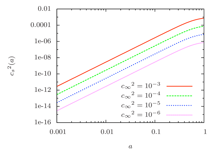
Figure 5: Sound speed ${c_{s}}^{2}(a)$ for different values of ${c_{\infty}}^{2}=10^{-6},10^{-5},10^{-4},10^{-3}$ from bottom to top (see [41]).

Figure 6: Normalized potentials $\Phi_{k}(a)/\Phi_{k}(0)$ are shown for $\Lambda$CDM (solid) and UDM (dot-dashed) (see [41]). The lower panel shows potentials at $k=0.001\,h\,\mathrm{Mpc}^{-1}$, the medium panel at $k=0.01\,h\,\mathrm{Mpc}^{-1}$ and the upper panel at $k=0.1\,h\,\mathrm{Mpc}^{-1}$. UDM curves are for ${c_{\infty}}^{2}=10^{-6},10^{-4},10^{-2}$ from top to bottom, respectively. At small $c_{\infty}$, $\Lambda$CDM and UDM curves are indistinguishable.

In Fig. 6 we present some Fourier components $\Phi_{k}(a)$ of the gravitational potential, normalized to unity at early times (see [41]). As we can note from this figure, the possible appearance of a sound speed significantly different from zero at late times corresponds to the appearance of a Jeans’ length under which the dark fluid does not cluster any more, causing a strong evolution in time of the gravitational potential. By increasing the sound speed, the potential starts to decay earlier in time, oscillating around zero afterwards. Moreover, at small scales, if the sound speed is small enough, UDM reproduces $\Lambda$CDM. This reflects the dependence of the gravitational potential on the effective Jeans’ length ${\lambda_{J}}(a)$ [32].

Finally, in Ref. [41] the authors show for this UDM model the lensing signal in linear theory as produced in $\Lambda$CDM and UDM; as sources, they consider the CMB and background galaxies, with different values of the peak and different shapes of their redshift distribution. For sound speed lower than $c_{\infty}=10^{-3}$, in the window of multipoles $l\gtrsim 10$ (Limber’s approximation) and where our ignorance on non–linear effects due to small scales dynamics become relevant, the power spectra of the cosmic convergence (or shear) in the flat–sky approximation in UDM and $\Lambda$CDM are similar. When the Jeans’ length $\lambda_{J}(a)$ increases, the Newtonian potential starts to decay earlier in time (at a fixed scale), or at greater scales (at a fixed epoch). This behaviour reflects on weak lensing by suppressing the convergence power spectra at high multipoles. They find that, for values of the sound speed between $c_{\infty}=10^{-3}$ and $c_{\infty}=10^{-2}$, UDM models are still comparable with $\Lambda$CDM, while for higher values of $c_{\infty}$ these models are ruled out because of the inhibition of structure formation. Moreover, they find that the dependence of the UDM weak lensing signal on the sound speed $c_{\infty}$ increases with decreasing redshift of the sources. They also show the errors for the fiducial $\Lambda$CDM signal for wide–field surveys like EUCLID or Pan–STARRS, and they find that one isin principle able to distinguish $\Lambda$CDM from UDM models when $c_{\infty}\gtrsim 10^{-2}$. Moreover, in Ref. [46] the authors calculate the 3D shear matrix $C^{\gamma\gamma}(k_{1},k_{2};\ell)$ in the flat-sky approximation for a large number of values of $c_{\infty}$. They see that, whilst the agreement with the $\Lambda$CDM model is good for small values of $c_{\infty}$, when one increases the sound speed parameter, the lensing signal appears more suppressed at small scales, and the 3D shear matrix shows bumps related to the oscillations of the gravitational potential. Moreover, they show that the expected evidence clearly shows that the survey data would unquestionably favour UDM models over the standard $\Lambda$CDM model, if its sound speed parameter exceed $10^{-4}$.

7.3 Prescription for UDM Models with a generic kinetic term

We now describe a general prescription to obtain a collection of models that reproduce a background similar to $\Lambda$CDM and have a suitable sound speed. Some comments about the master equation (108) are first necessary. The relation (108) enables to determine a connection between the scalar factor $a$ and the kinetic term $X$ on the manifold $\mathcal{M}_{\Lambda}$ and therefore a mapping between the cosmic time and the manifold $\mathcal{M}_{\Lambda}$.

Now it is easy to see that the LHS of Eq. (108), seen as a single function of $X$, must have at least a vertical asymptote and a zero, and the function must be continuous between the two. In particular, when $X$ is near the vertical asymptote the universe approaches the cosmological constant regime, whereas when $X$ is close to the zero of the function, the dark fluid behaves like dark matter. Therefore, if we define

$$f(\varphi(X))=\frac{\mathcal{F}(X)}{2X(\partial g(X)/\partial X)}$$ (119)

where, for example,

$$\mathcal{F}(X)=\frac{1}{\mu}\frac{X_{f}-X}{X-X_{i}}\;,$$ (120)

(where $\mu$ is an appropriate positive constant) the value of $X_{f}$ and $X_{i}$ are the zero and the asymptote mentioned above, namely, when $a\rightarrow 0$ we have $X\rightarrow X_{i}$ and when $a\rightarrow\infty$ we have $X\rightarrow X_{f}$. Moreover, if $X_{f}>X_{i}$ we have $dX/dN>0$, whereas if $X_{f}<X_{i}$ we have $dX/dN<0$. In other words, according to Eq.(108),

$$X(a)=X_{f}\frac{1+(X_{i}/X_{f})\Lambda\mu\nu~{}a^{-3}}{1+\Lambda\mu\nu~{}a^{-3}}\;.$$ (121)

Let us emphasize that the values of $X_{i}$ and $X_{f}$ are very important because they automatically set the range of values that the sound speed can assume at the various cosmic epochs.

Let us finally make another important comment. One can use this reconstruction of the UDM model in the opposite way. In fact, by imposing a cosmological background identical to $\Lambda$CDM, the observed CMB power spectrum, and the observed evolution of cosmic structures, one can derive the evolution of the sound speed $c_{s}^{2}$ vs. cosmic time. In this case, by assuming an appropriate kinetic term $g(X)$ through Eq. (105), we can derive $X(a)$ and, consequently, $\varphi(a)$ and $X(a(\varphi))=X(\varphi)$. Therefore, by using the relations (108) and $V(\varphi)=f(\varphi)g(X)+\Lambda$, one can determine the functional form of $f(\varphi)$ and $V(\varphi)$.

8 Generalized UDM Models

In this Section we consider several possible generalizations of the technique introduced in Section 7.1, with the aim of studying models where the background does not necessarily mimic the $\Lambda$CDM background (see [38, 49]).

Let us consider a scalar field Lagrangian $\mathcal{L}$ of the form

$$\mathcal{L}(X,\varphi)=p(\varphi,X)=f(\varphi)g(h(\varphi)X)-V(\varphi)\;.$$ (122)

Note that, introducing the three potentials $f(\varphi)$, $h(\varphi)$ and $V(\varphi)$, we follow an approach similar to the one studied in Ref. [38] in order to decouple the equation of state parameter $w$ and the sound speed $c_{\rm s}$. In order to reconstruct these potentials we need three dynamical conditions: $a)$ a choice for $p(N)$, $b)$ the continuity equation or, equivalently, the equation of motion (11), $c)$ a choice for $c_{s}^{2}(N)$ (see [49]).

Let us obtain the Lagrangian through two different simple approaches:

• By choosing $p(N)$. Indeed we get

  $$\frac{d\rho}{dN}+3\rho=-3p(N)\;,\quad\quad{\rm i.e.}\quad\quad\rho(N)=e^{-3N}\left[-3\int^{N}\left(e^{3N^{\prime}}p(N^{\prime})dN^{\prime}\right)+K\right]\;,$$ (123)

  where $K$ is an integration constant. By imposing the condition $\mathcal{L}(X,\varphi)=p(N)$ along the classical trajectories, we obtain $\varphi=\mathcal{L}^{-1}(X(N),p(N))\big{|}_{\mathcal{M}_{p(N)}}$. Thus, starting from a generic Lagrangian $\mathcal{L}=f(\varphi)g(h(\varphi)X)-V(\varphi)$ we get

  $$2X(N)\left[\frac{\partial g(h(\varphi[X,N])X)}{\partial X}\right](N)f(\varphi(X,N))=p(N)+e^{-3N}\left[-3\int^{N}\left(e^{3N^{\prime}}p(N^{\prime})dN^{\prime}\right)+K\right]\;.$$ (124)

  For example, if $p=-\Lambda$, $K=\rho(a=1)-\Lambda$. The freedom provided by the choice of $K$ is particularly relevant. In fact, by setting $K=0$, we can remove the term $\rho\propto a^{-3}$. Alternatively, when $K\neq 0$, we always have a term that behaves like presseure-less matter. We thus show that the single fluid of UDM models can mimic not only a cosmological constant but also any quintessence fluid.

  Thus, using Eq. (124) and following the procedure described in Section 7.1, one gets the relations $X\equiv\mathcal{G}_{p}(N)$, and consequently

  $$\varphi \equiv \mathcal{Q}_{p}(N)=\varphi_{0}$$ (125)

  $$\pm \int^{N}\left\{\mathcal{G}_{p}(N^{\prime})^{1/2}\left[-3e^{-3N}\int^{N}\left(e^{3N^{\prime}}p(N^{\prime})dN^{\prime}\right)+Ke^{-3N}\right]^{-1/2}dN^{\prime}\right\}\;.$$

  Therefore, with the functions $\mathcal{G}_{p}(N)$ and $\mathcal{Q}_{p}(N)$, one can write $f(X,N)=f(\mathcal{G}_{p}(N),N)=f(\mathcal{G}_{p}(\mathcal{Q}_{p}^{-1}(\varphi)),\mathcal{Q}_{p}^{-1}(\varphi))=f(\varphi)$. Thus, by starting from a Lagrangian whose behavior is given by $p(N)$, the speed of sound is determined by the appropriate choice of $g(h(\varphi)X)$, where $h(X,N)=h(\mathcal{G}_{p}(N),N)=h(\mathcal{G}_{p}(\mathcal{Q}_{p}^{-1}(\varphi)),\mathcal{Q}_{p}^{-1}(\varphi))=h(\varphi)$.

• By choosing the equation of state $w(N)$. Indeed

  $$\rho(N)=\rho_{0}e^{-3\int^{N}(w(N^{\prime})+1)dN^{\prime}}\;,$$ (126)

  where $\rho_{0}$ is a positive integration constant, and

  $$p(N)=\rho_{0}w(N)e^{-3\int^{N}(w(N^{\prime})+1)dN^{\prime}}\;.$$ (127)

  Therefore, still by imposing the condition $\mathcal{L}(X,\varphi)=p[w(N),N]$ along the classical trajectories, i.e. $\varphi=\mathcal{L}^{-1}[X(N),p(w(N),N)]\big{|}_{\mathcal{M}_{w(N)}}$, one gets

  $$2X\frac{\partial g(h(\varphi[X,N])X)}{\partial X}f(X,N)=\rho_{0}[w(N)+1]e^{-3\int^{N}(w(N^{\prime})+1)dN^{\prime}}\;.$$ (128)

  Therefore, on the classical trajectory we can impose, by using $w(N)$, a suitable function $p(N)$ and thus the function $\rho(N)$. The master equation Eq. (128) generalizes Eq. (108). Also in this case, by Eq. (128) and by following the argument described in Section 7.1, one can get the relations $X\equiv\mathcal{G}_{w}(N)$, and consequently

  $$\varphi\equiv\mathcal{Q}_{w}(N)=\pm\int^{N}\left\{\mathcal{G}_{w}(N^{\prime})^{1/2}\left[\rho_{0}e^{-3\int^{N^{\prime}}(w(N^{\prime\prime})+1)dN^{\prime\prime}}\right]^{-1/2}dN^{\prime}\right\}+\varphi_{0}\;.$$ (129)

  Thus, with the functions $\mathcal{G}_{w}(N)$ and $\mathcal{Q}_{w}(N)$, one can write $f(X,N)=f(\mathcal{G}_{w}(N),N)=f(\mathcal{G}_{w}(\mathcal{Q}_{w}^{-1}(\varphi)),\mathcal{Q}_{w}^{-1}(\varphi))=f(\varphi)$. Then we can find a Lagrangian whose behavior is determined by $w(N)$ and whose speed of sound is determined by the appropriate choice of $g(h(\varphi)X)$, where $h(X,N)=h(\mathcal{G}_{p}(N),N)=h(\mathcal{G}_{p}(\mathcal{Q}_{p}^{-1}(\varphi)),\mathcal{Q}_{p}^{-1}(\varphi))=h(\varphi)$.

Let us conclude that the $p(N)$ constraint on the equation of motion is actually a weaker condition than the $w(N)$ constraint. The larger freedom that the $p(N)$ constraint provides naturally yields an additive term in the energy density that decays like $a^{-3}$, i.e. like a matter term in the homogeneous background. Let us emphasize that this important result is a natural consequence of the $p(N)$ constraint and is not imposed a priori (see [38, 49]).

9 Halos of Unified Dark Matter Scalar Field

A complete analysis of UDM models should necessarily include the study of static solutions of Einstein’s field equations. This is complementary to the study of cosmological background solutions and would allow to impose further constraints to the Lagrangian of UDM models. The authors of Refs. [123] and [95] have studied spherically symmetric and static configuration for k-essence models. In particular, they studied models where the rotation velocity becomes flat (at least) at large radii of the halo. In these models the scalar field pressure is not small compared to the mass-energy density, similarly to what is found in the study of general fluids in Refs. [124, 125, 126, 127], and the Einstein’s equations of motion do not reduce to the equations of Newtonian gravity. Further alternative models have been considered, even with a canonical kinetic term in the Lagrangian, that describe dark matter halos in terms of bosonic scalar fields, see e.g. Refs. [128, 66, 67, 68, 21, 63, 64, 65, 129, 130].
In this Section we assume that our scalar field configurations only depend on the radial direction. Three main results are achieved. First, we are able to find a purely kinetic Lagrangian which allows simultaneously to provide a flat rotation curve and to realize a unified model of dark matter and dark energy on cosmological scales. Second, an invariance property of the expression for the halo rotation curve is found. This allows to obtain purely kinetic Lagrangians that reproduce the same rotation curves that are obtained starting from a given density profile within the standard Cold Dark Matter (CDM) paradigm. Finally, we consider a more general class of models with non-purely kinetic Lagrangians. In this case one can extend to the static and spherically symmetric spacetime metric the procedure used in Ref. [33] to find UDM solutions in a cosmological setting. Such a procedure requires that the Lagrangain is constant along the classical trajectories; we are thus able to provide the conditions to obtain reasonable rotation curves within a UDM model of the type discussed in Ref. [33].

9.1 Static solutions in Unified Dark Matter models

Let us consider a scalar field which is static and spatially inhomogeneous, i.e. such that $X<0$. In this situation the energy-momentum tensor is not described by a perfect fluid and its stress energy-momentum tensor reads

$$T^{\varphi}_{\mu\nu}=(p_{\parallel}+\rho)n_{\mu}n_{\nu}-\rho g_{\mu\nu}$$ (130)

where

$$\rho=-p_{\perp}=-\mathcal{L}\;,$$ (131)

$n_{\mu}=\nabla_{\mu}\varphi/\sqrt{-2X}$ and $p_{\parallel}=\mathcal{L}-2X\partial\mathcal{L}/\partial X$. In particular, $p_{\parallel}$ is the pressure in the direction parallel to $n_{\mu}$ whereas $p_{\perp}$ is the pressure in the direction orthogonal to $n_{\mu}$. It is simpler to work with a new definition of $X$. Indeed, defining $X=-\chi$ we have

$$n_{\mu}=\nabla_{\mu}\varphi/(2\chi)^{1/2}$$ (132)

$$p_{\parallel}=2\chi\frac{\partial\rho}{\partial\chi}-\rho\;.$$ (133)

Let us consider for simplicity the general static spherically symmetric spacetime metric i.e.

$$ds^{2}=-\exp{(2\alpha(r))}\;dt^{2}+\exp{(2\beta(r))}\;dr^{2}+r^{2}d\Omega^{2}\,,$$ (134)

where $d\Omega^{2}=d\theta^{2}+\sin^{2}\theta d\phi^{2}$ and $\alpha$ and $\beta$ are two functions that only depend upon $r$.
As the authors of Refs. [123, 95] have shown, it is easy to see that the non-diagonal term $T^{rt}$ vanishes. Therefore $\varphi$ could be either strictly static or depend only on time. In this section we study the solutions where $\varphi$ depends on the radius only.

In the following we will consider some cases where the baryonic content is not negligible in the halo. In this case we will assume that most of the baryons are concentrated within a radius $r_{b}$. If we define $M_{*}$ as the entire mass of the baryonic component then for $r>r_{b}$ we can simply assume that $M_{*}$ is concentrated in the center of the halo.

Considering, therefore, the halo for $r>r_{b}$, starting from the Einstein’s equations and the covariant conservation of the stress-energy (or from the equation of motion of the scalar field, Eq. (4)), we obtain

$$\frac{1}{r^{2}}\left\{1-\left[r\exp{\left(-2\beta\right)}\right]^{\prime}\right\}=\rho \Longleftrightarrow \frac{dM}{dr}=4\pi\rho r^{2}\;,$$ (135)

$$\frac{1}{r^{2}}\left\{\exp{\left[-2(\alpha+\beta)\right]}\left[r\exp{\left(2\alpha\right)}\right]^{\prime}-1\right\}=p_{\parallel} \Longleftrightarrow \alpha^{\prime}=\frac{\frac{M+M_{*}}{8\pi}+\frac{p_{\parallel}r^{3}}{2}}{r^{2}\left[1-\frac{M+M_{*}}{4\pi r}\right]}\;,$$

$$\frac{\exp{\left[-(\alpha+2\beta)\right]}}{r}\left\{\left[r\exp{\alpha}\right]^{\prime}\beta^{\prime}-\left[r\left(\exp{\alpha}\right)^{\prime}\right]^{\prime}\right\}=\rho\;,$$ (137)

$$\frac{dp_{\parallel}}{dR}=-(p_{\parallel}+\rho)$$ (138)

(which are the $00$, $rr$ and $\theta\theta$ components of Einstein’s equations and the $r$ component of the continuity equation respectively) where

$$\exp{(-2\beta(r))}=1-(M+M_{*})/(4\pi r)$$

and

$$R=\ln[r^{2}\exp(\alpha(r))]$$

, where a prime indicates differentiation with respect to the radius $r$.

A first comment is in order here. If i) $\beta^{\prime}=0$ and ii) $\left[r\left(\exp{\alpha}\right)^{\prime}\right]^{\prime}>0$, then we can immediately see that $\rho<0$. These conditions must therefore be avoided when trying to find a reasonable rotation curve. For example, neglecting the baryonic mass, the special case of $\rho=A/r^{2}$ and $\exp(\alpha)\sim r^{m}$, where $A$ and $m$ are constants, fall into this case. One thus recovers the no-go theorem derived in Ref. [95] under the assumption that the rotation curve $v_{c}\ll 1$ is constant for all $r$.
The value of the circular velocity $v_{c}$ is determined by the assumption that a massive test particle is also located at $\theta=\pi/2$. We define as massive test particle the object that sends out a luminous signal to the observer who is considered to be stationary and far away from the halo.

Considering the motion of a massive test particle, say a star, in a such a halo, its trajectory is then described by a curve $x^{\mu}=(t,r,\theta,\phi)$ parameterized by some affine parameter; here we use its proper time $\tau$. Its four velocity is then simply $u^{\mu}\equiv dx^{\mu}/d\tau$. Due to spherical symmetry, we can assume without loss of generality that the star’s ecliptic is located in the $\theta=\pi/2$ plane. Since the star is a massive particle, its norm is $u_{\mu}u^{\mu}=-1$, which becomes the constraint equation

$$\exp{(2\alpha)}\dot{t}^{2}-\exp{(2\beta)}\dot{r}^{2}-r^{2}\dot{\phi}^{2}=1,$$ (139)

where a dot denotes a derivative with respect to proper time $\tau$. Since the metric does not explicitly depend on $\theta$, the star’s angular momentum $l$ is conserved,

$$l=r^{2}\dot{\phi}.$$ (140)

Similarly, the metric does not explicitly depend on $t$, and there is a conserved energy $E$,

$$E=\exp{(2\alpha)}\dot{t}.$$ (141)

Substituting equations (141) and (140) into equation (139), one finds a first integral of motion for the star,

$$\frac{1}{2}\dot{r}^{2}+\mathcal{V}(r)=0,$$ (142)

where its effective potential is

$$\mathcal{V}(r)=\frac{1}{2}\exp{(-2\beta)}\left(1+\frac{l^{2}}{r^{2}}\right)-\frac{1}{2}E^{2}\exp{[-2(\alpha+\beta)]}.$$ (143)

Note that the potential explicitly depends on the energy. Stationary orbits at radius $r$ exist if $\mathcal{V}$ and $d\mathcal{V}/dr$ vanish at that radius. The former condition yields

$$1+\frac{l^{2}}{r^{2}}=E^{2}\exp{[-2\alpha(r)]},$$ (144)

whereas the latter gives us

$$-\beta^{\prime}\left(1+\frac{l^{2}}{r^{2}}\right)-\frac{l^{2}}{r^{3}}+E^{2}\left(\alpha^{\prime}+\beta^{\prime}\right)\exp{[-2\alpha(r)]}=0.$$ (145)

Substituting equation (144) into equation (145) and using the Eqs. (135), (9.1) and (4), we get the following equation

$$\frac{l^{2}/r^{2}}{1+l^{2}/r^{2}}=\frac{(M+M_{*})(r)}{8\pi r}+r^{2}\,\frac{p_{\parallel}(r)}{2},$$ (146)

which directly relates the angular momentum $l$ to the density profile of the halo.

In this case, through the definition of the star’s angular momentum $l$ and Eq. (146), the value of $v_{c}\equiv l/r$ can be rewritten as

$$v_{c}^{2}=\frac{p_{\parallel}r^{2}/2+(M+M_{*})/(8\pi r)}{1-\left[p_{\parallel}r^{2}/2+(M+M_{*})/(8\pi r)\right]}\;,$$ (147)

but when we consider the weak-field limit condition $(M+M_{*})/(8\pi r)\ll 1$ and since the rotation velocities of the halo of a spiral galaxy are typically non-relativistic, $v_{c}\ll 1$, Eq. (147) simplifies to [123]

$$v_{c}^{2}\approx\frac{M+M_{*}}{8\pi r}+\frac{p_{\parallel}r^{2}}{2}\;.$$ (148)

A second comment follows from the fact that the pressure is not small compared to the mass-energy density. In other words we do not require that general relativity reduces to Newtonian gravity (see also Refs. [124, 125, 126, 127]). Notice also that in the region where $v_{c}\approx{\rm const.}\ll 1$ it is easy to see that in general $\exp(\alpha)\approx{\rm const.}$ since from Eqs. (9.1) and (148) one obtains $r\alpha^{\prime}\approx v_{c}^{2}$.

Finally, let us point out one of the main results (see also Ref.  [38]). We can see that the relation (148) is invariant under the following transformation

$$\rho\longrightarrow\widetilde{\rho}=\rho+\sigma(r)\quad\quad\quad p_{\parallel}\longrightarrow\widetilde{p_{\parallel}}=p_{\parallel}+q(r)$$ (149)

if

$$3q(r)+rq(r)^{\prime}=-\sigma(r)\;,$$ (150)

up to a proper choice of some integration constants. Thanks to this transformation we can consider an ensemble of solutions that have the same rotation curve. Obviously, these solutions have to satisfy Einstein’s equations (135), (9.1) and (137), and the covariant conservation of the stress-energy (138). Moreover, we will require the validity of the weak energy conditions, $\rho\geq 0$ and $p_{\parallel}+\rho\geq 0$, i.e.

$$2\frac{\exp{\left(-2\beta\right)}}{r}(\alpha^{\prime}+\beta^{\prime})=2\chi\frac{\partial\rho}{\partial\chi}\geq 0\;.$$ (151)

9.2 Unified Dark Matter models with purely kinetic Lagrangians

Let us consider a scalar field Lagrangian $\mathcal{L}$ with a non-canonical kinetic term that depends only on $X$ or $\chi$. Moreover, in this section we assume that $M_{*}=0$ (or $M\gg M_{*}$).

First of all we must impose that $\mathcal{L}$ is negative when $X<0$, so that the energy density is positive. Therefore, we define a new positive function

$$g_{s}(\chi)\equiv-\mathcal{L}(X)\;.$$ (152)

As shown in Ref. [123], when the equation of state $p_{\parallel}=p_{\parallel}(\rho)$ is known, one can write the purely kinetic Lagrangian that describes this dark fluid with the help of Eqs. (131) and (133). Alternatively, using (138), one can connect $p_{\parallel}$ and $\rho$ in terms of $r$ through the variable $R$. Moreover, it is easy to see that starting from the field equation of motion (4), there exists another relation that connects $\chi$ (i.e. $X$) with $r$. This relation is

$$\chi\left[\frac{dg_{s}(\chi)}{d\chi}\right]^{2}=\frac{k}{\left[r^{2}\exp{\alpha(r)}\right]^{2}}$$ (153)

with $k$ a positive constant. If we add an additive constant to $g_{s}(\chi)$, the solution (153) remains unchanged. One can see this also through Eq. (138). Indeed, using Eqs. (131) and  (133) one immediately finds that Eq. (138) is invariant under the transformation $\rho\rightarrow\rho+K$   $p_{\parallel}\rightarrow p_{\parallel}-K$. In this way we can add the cosmological constant $K=\Lambda$ to the Lagrangian and we can describe the dark matter and the cosmological constant-like dark energy as a single dark fluid i.e. as Unified Dark Matter (UDM).

Let us notice that one can adopt two approaches to find reasonable rotation curves $v_{c}(r)$. A static solution can be studied in two possible ways:

• The first approach consists simply in adopting directly a Langrangian that provides a viable cosmological UDM model and exploring what are the conditions under which it can give a static solution with a rotation curve that is flat at large radii. This prescription has been already applied, for example, in Ref. [123].

• A second approach consists in exploiting the invariance property of Eq. (148), with respect to the transformation (149) (when the condition (150) is satisfied). Usually in the literature one reduces the problem to the Newtonian gravity limit, because one makes use of a CDM density profile, i.e. one assumes that in Eq. (148), $p_{\parallel}\ll M/(4\pi r^{3})$. We can therefore use Eqs. (149) and (150) to obtain energy density and pressure profiles $\rho(r)$ and $p_{\parallel}(r)$ that reproduce the same rotation curve in a model with non-negligible pressure. Next, we find an acceptable equation of state $p_{\parallel}=p_{\parallel}(\rho)$ such that we can reconstruct, through Eqs. (131) and (133), the expression for the Lagrangian $\mathcal{L}$. Such a procedure establishes a mapping between UDM and CDM solutions that predict the same halo rotation curve $v_{c}(r)$. As a starting point we could, of course, use very different CDM density profiles to this aim, such as the modified isothermal-law profile [131], the Burkert profile [132], the Moore profile [133], the Navarro-Frenk-White profile [134, 135] or the profile proposed by Salucci et al. (see for example [136, 137, 138, 139]).
  As we have already mentioned, the possible solutions one finds in this way have to satisfy the Einstein equations (135), (9.1) and (137), the conservation of stress-energy (138) and the weak energy conditions. Moreover, the resulting UDM scalar field Lagrangian must be able to provide cosmological solutions that yield an acceptable description of the cosmological background (see, e.g., Ref. [33]) and low effective speed of sound (see for example Refs. [70, 100, 32]) so that cosmic structure formation successfully takes place and CMB anisotropies fit the observed pattern [27, 31, 25, 28].

Below, using approach i), we provide a worked example of a UDM model with purely kinetic Lagrangian which is able to describe a flat halo rotation curve and then, using approach ii), we give a general systematic procedure to obtain a possible Lagrangian of UDM model starting from a given CDM density profile.

9.2.1 Approach i): The generalized Scherrer solution

Let us consider the generalized Scherrer solution models obtained in Ref. [33] (see also Sect. 4.3). These models are described by the following Lagrangian

$$\mathcal{L}=-\Lambda+g_{n}\left(X-\hat{X}\right)^{n}$$ (154)

where $g_{n}>0$ is a suitable constant and $n>1$. The case $n=2$ corresponds to the unified model proposed by Scherrer  [30]. If we impose that today $[(X-\hat{X})/\hat{X}]^{n}\ll 1$, the background energy density can be written as

$$\rho(a(t))=\rho_{\Lambda}+\rho_{\rm DM}\;,$$ (155)

where $\rho_{\Lambda}$ behaves like a “dark energy” component ($\rho_{\Lambda}={\rm const.}$) and $\rho_{\rm DM}$ behaves like a “dark matter” component i.e. $\rho_{\rm DM}\propto a^{-3}$, with $a(t)$ the scale factor.
A static solution for the generalized Scherrer model can be obtained in two possible ways:

• Starting from the analysis of Ref. [95], in the case of a barotropic Lagrangian for the homogeneous field. The authors of Ref. [95] indeed concluded that for $n\gg 1$ flat halo rotation curves can be obtained. In particular they studied spherically symmetric solutions with the following metric,

  $$ds^{2}=-\left(\frac{r}{r_{\star}}\right)^{b}dt^{2}+N(r)dr^{2}+r^{2}d\Omega^{2}.$$ (156)

  where $r_{\star}$ is a suitable length-scale and $b=2v_{c}^{2}$. In the trivial case where $N(r)$ is constant they find $\mathcal{L}(X)\propto X^{2/b}$ with $b\ll 1$. For $X\gg\hat{X}$ the Lagrangian $\mathcal{L}=-\Lambda+g_{n}(X-\hat{X})^{n}$ takes precisely this form.

• In the analysis of Ref. [123], solutions where $\varphi$ is only a function of the radius are considered. When the Lagrangian has the form $\mathcal{L}\propto X^{n}$, with $n\sim 10^{6}$ the halo rotation curve becomes flat at large radii. In this case $n$ must be an odd natural number, such that the energy density is positive. Our model is able to reproduce this situation when the matter density is large, i.e. when $|X|\gg\hat{X}$.

Alternatively, if we wish to avoid large $n$ (c.f. case 2) above) we can start from the following Lagrangian

$$\mathcal{L}=-\Lambda+\epsilon_{X}g_{n}\left(|X|-\hat{X}\right)^{n}$$ (157)

where $\epsilon_{X}$ is some differentiable function of $X$ that is $1$ when $X\geq\hat{X}$ and $-1$ when $X\leq-\hat{X}<0$. In this way when $X>\hat{X}>0$ we recover the Lagrangian of the generalized Scherrer solutions. When $X<0$ and $\chi=-X>\hat{X}$ we get

$$\mathcal{L}=-\Lambda-g_{n}\left(\chi-\hat{X}\right)^{n}$$ (158)

and, with the help of Eqs. (131) and (133), we obtain

$$\rho=-p_{\perp}=-\mathcal{L}\;,\quad\quad\quad p_{\parallel}=(2n-1)g_{n}\left(\chi-\hat{X}\right)^{n}+2ng_{n}\hat{X}\left(\chi-\hat{X}\right)^{n-1}-\Lambda\;.$$ (159)

Now, requiring that $\chi$ be close to $\hat{X}$ (i.e. $\left(\chi-\hat{X}\right)\ll\hat{X}$) and $2ng_{n}\hat{X}\left(\chi-\hat{X}\right)^{n-1}\gg O(\Lambda)$, and starting from the relation (153) that connects $\chi$ with $r$, we get

$$\left(\chi-\hat{X}\right)^{n-1}=\frac{k^{1/2}}{ng_{n}\hat{X}^{1/2}}\;\frac{1}{r^{2}\exp{(\alpha(r))}}\;.$$ (160)

Consistency with our approximations implies that we have to consider the following expressions for radial configurations with $r$ bigger than a minimum radius $r_{min}$. In this case $p_{\parallel}$ and $\rho$ become

$$p_{\parallel}=\frac{A}{r^{2}\exp{(\alpha(r))}}\;,\quad\quad\quad\rho=\frac{B}{[r^{2}\exp{(\alpha(r))}]^{n/(n-1)}}$$ (161)

where $A=2(k\hat{X})^{1/2}$ and $B=g_{n}\left[k^{1/2}/(ng_{n}\hat{X}^{1/2})\right]^{n/(n-1)}$.

Using Eqs. (135) and (9.1), one can calculate the values of the metric terms $\exp{(\alpha)}$ and $\exp{(\beta)}$ and, thus the value of $\rho$ and $p_{\parallel}$. Alternatively we know that when $v_{c}\approx{\rm const.\ll 1}$ at large radii, in a first approximation, we can set $\exp(\alpha(r))\approx C=$ const. Therefore for $n\neq 3$, we can write the function $M$ as

$$M(r)\approx\frac{4\pi B}{C^{n/(n-1)}}\left(\frac{n-1}{n-3}r^{\frac{n-3}{n-1}}+D\right)$$ (162)

where we could also set $D=0$ for $n>3$. Instead, when $1<n<3$, the second term has to be larger than the first one.

In these cases $v_{c}^{2}$ becomes

$$v_{c}^{2}(r)\approx\frac{A}{2C}+\frac{B}{2\;C^{n/(n-1)}}\left(\frac{n-1}{n-3}\frac{1}{r^{2/(n-1)}}+\frac{D}{r}\right)\;.$$ (163)

For $n=3$ we have

$$M(r)\approx\frac{4\pi B}{C^{3/2}}\ln\left(\frac{r}{\bar{r}}\right)+M(\bar{r})$$ (164)

where $r>\bar{r}$ and

$$v_{c}^{2}\approx\frac{A}{2C}+\frac{B}{2\;C^{3/2}}\frac{1}{r}\ln\left(\frac{r}{\bar{r}}\right)+\frac{M(\bar{r})}{8\pi r}\;.$$ (165)

In other words we see that the circular velocity becomes approximately constant for sufficiently large $r$.

However, let us stress that $\exp(\alpha(r))$ cannot be strictly constant, and that it should be chosen in such a way that the positivity of Eq. (137) is ensured.

This example can be generalized also to $M_{*}\neq 0$. Obviously, in such a case we have to assume that $r>r_{b}\geq r_{min}$. In this case $k$, $r_{min}$, $A$, $B$ (through $\exp(\beta(r))$) and $C$ depend on $M_{*}$.

The spherical top-hat solution for this model, which provides the link with the cosmological initial conditions, is described in the Sect. A.

9.3 Approach ii): A general prescription to obtain UDM Lagrangians starting from a profile of an energy density distribution of CDM

Defining the energy density distribution of CDM as $\rho_{\rm CDM}(r)$ (with $p_{\rm CDM}=0$), the transformation (149) becomes

$$\rho(r)=\rho_{\rm CDM}(r)+\sigma(r)\,,\quad\quad\quad p_{\parallel}(r)=q(r)\;.$$ (166)

Now, starting from a given CDM density profile, through Eqs. (135), (9.1), (138) and (150) we can determine $\exp{(\alpha)}$ ,  $\exp{(\beta)}$,  $\rho$  and  $p_{\parallel}$. In a second step we provide the conditions to ensure that the energy density is positive . In this case, after some simple but lengthy calculations, one finds

$$\mathcal{Q}^{\prime}(r)\left(r\frac{M_{\rm CDM}(r)}{4\pi}-2r\mathcal{Q}(r)\right) - 2\mathcal{Q}^{2}(r)$$

$$+\mathcal{Q}(r)\left(4r+3\frac{M_{\rm CDM}(r)}{4\pi}+4r^{3}\rho_{\rm CDM}\right) = \frac{rM_{\rm CDM}(r)}{4\pi}\left(4+3r^{2}\rho_{\rm CDM}\right)\;,$$

$$\mathcal{B}(r) = \mathcal{Q}(r)-\frac{M_{\rm CDM}(r)}{4\pi}\;,$$ (168)

$$\mathcal{A}(r) = \frac{\mathcal{Q}(r)+\mathcal{B}(r)}{2\mathcal{B}(r)}\;,$$ (169)

$$\sigma(r) = \frac{1-\mathcal{Q}^{\prime}(r)}{r^{2}}$$ (170)

where $\mathcal{Q}(r)=r(r^{2}q+1)$ ,  $\mathcal{B}(r)=r\exp{(-2\beta)}$ and $\mathcal{A}(r)=(r\alpha^{\prime}+1)$. Here we define $M_{\rm CDM}(r)=4\pi\int_{0}^{r}\tilde{r}^{2}\rho_{\rm CDM}(\tilde{r})~{}d\tilde{r}$. At this point it is easy to see that Eq. (9.3) does not admit a simple analytical solution for a generic $\rho_{\rm CDM}$. On the other hand we know that, through $\rho_{\rm CDM}$, all these functions depend on the velocity rotation curve $v_{c}(r)$. Moreover $v_{c}^{2}(r)\ll 1$. Therefore, defining $\bar{v}_{c}$ as the value that $v_{c}$ assumes when the rotation curve is flat at large radii or the maximum value of $v_{c}$ with a particular profile of $\rho_{\rm CDM}$, one can expand $\mathcal{Q}$, $\mathcal{A}$ and $\mathcal{B}$ as

$$\mathcal{Q}(r) = \mathcal{Q}_{(0)}(r)+\bar{v}_{c}^{2}\mathcal{Q}_{(1)}(r)+\frac{\left(\bar{v}_{c}^{2}\right)^{2}}{2!}\mathcal{Q}_{(2)}(r)+\dots\;,$$

$$\mathcal{A}(r) = \mathcal{A}_{(0)}(r)+\bar{v}_{c}^{2}\mathcal{A}_{(1)}(r)+\frac{\left(\bar{v}_{c}^{2}\right)^{2}}{2!}\mathcal{A}_{(2)}(r)+\dots\;,$$

$$\mathcal{B}(r) = \mathcal{B}_{(0)}(r)+\bar{v}_{c}^{2}\mathcal{B}_{(1)}(r)+\frac{\left(\bar{v}_{c}^{2}\right)^{2}}{2!}\mathcal{B}_{(2)}(r)+\dots\;.$$ (171)

Following this procedure one can determine $\rho$ and $p_{\parallel}$ in a perturbation way, i.e.

$$\rho(r)=\rho_{(0)}(r)+\bar{v}_{c}^{2}\rho_{(1)}(r)+\frac{\left(\bar{v}_{c}^{2}\right)^{2}}{2!}\rho_{(2)}(r)+\dots\;,$$ (172)

$$p_{\parallel}(r)=p_{\parallel\;(0)}(r)+\bar{v}_{c}^{2}p_{\parallel\;(1)}(r)+\frac{\left(\bar{v}_{c}^{2}\right)^{2}}{2!}p_{\parallel\;(2)}(r)+\dots\;.$$ (173)

Now, looking at the various CDM density profiles which have been proposed in the literature [131, 132, 133, 134, 135, 139], we see that one can always take $\rho_{\rm CDM}$ as

$$\rho_{\rm CDM}(r)=\bar{v}_{c}^{2}\rho_{{\rm CDM}\;(1)}(r)\;,$$ (174)

then

$$M_{\rm CDM}(r)=\bar{v}_{c}^{2}M_{{\rm CDM}\;(1)}(r)=4\pi~{}\bar{v}_{c}^{2}\int_{0}^{r}\tilde{r}^{2}\rho_{{\rm CDM}\;(1)}(\tilde{r})~{}d\tilde{r}\;.$$ (175)

For the zeroth-order terms one immediately obtains

$$\mathcal{Q}_{(0)} = r\;,$$

$$\mathcal{A}_{(0)} = 1\;,$$

$$\mathcal{B}_{(0)} = r\;.$$ (176)

At the first order one gets

$$\mathcal{Q}_{(1)} = \frac{2}{r}\int_{0}^{r}\tilde{r}^{3}\rho_{{\rm CDM}\;(1)}(\tilde{r})~{}d\tilde{r}\;,$$

$$\mathcal{A}_{(1)} = \frac{1}{2r}\frac{M_{{\rm CDM}\;(1)}(r)}{4\pi}\;,$$

$$\mathcal{B}_{(1)} = \frac{2}{r}\int_{0}^{r}\tilde{r}^{3}\rho_{{\rm CDM}\;(1)}(\tilde{r})~{}d\tilde{r}-\frac{M_{{\rm CDM}\;(1)}(r)}{4\pi}\;.$$ (177)

For completeness we write also the second order for $\mathcal{Q}$

$$\mathcal{Q}_{(2)}=\frac{1}{r}\int_{0}^{r}d\check{r}\frac{M_{{\rm CDM}\;(1)}(\check{r})}{4\pi}\left[\frac{2}{\check{r}}\mathcal{Q}_{(1)}({\check{r}})-{\check{r}}^{2}\rho_{{\rm CDM}\;(1)}({\check{r}})\right]\,.$$ (178)

Let us stress that if one considers also terms $O\left(\bar{v}_{c}^{4}\right)$, Eq. (147) instead of Eq. (148) should be used. In such a case, $v_{c}$ slightly changes with respect to the velocity rotation curve that one obtains using a CDM density profile.

For our purposes we can consider only the zeroth and the first-order terms. At this point, one can finally calculate the value of  $\rho$  and  $p_{\parallel}$. One gets

$$\rho(r)=\rho_{\rm CDM}(r)+\frac{1-\mathcal{Q}^{\prime}(r)}{r^{2}}=\bar{v}_{c}^{2}\left(\frac{2}{r^{4}}\int_{0}^{r}\tilde{r}^{3}\rho_{{\rm CDM}\;(1)}(\tilde{r})~{}d\tilde{r}-\rho_{\rm CDM\;(1)}(r)\right)\;,$$ (179)

$$p_{\parallel}(r)=\frac{\mathcal{Q}(r)-r}{r^{3}}=\bar{v}_{c}^{2}\frac{2}{r^{4}}\int_{0}^{r}\tilde{r}^{3}\rho_{{\rm CDM}\;(1)}(\tilde{r})~{}d\tilde{r}\;.$$ (180)

As far as the values of the metric terms $\exp{(\alpha)}$ and $\exp{(\beta)}$ are concerned, we obtain the following expressions

$$\exp{(2\alpha)}=\exp{(2\alpha(\hat{r}))}\exp{\left[\bar{v}_{c}^{2}\int_{\hat{r}}^{r}\frac{1}{\tilde{r}^{2}}\frac{M_{{\rm CDM}\;(1)}(\tilde{r})}{4\pi}~{}d\tilde{r}\right]}$$ (181)

$$\exp{(-2\beta)}=1+\frac{\bar{v}_{c}^{2}}{r^{2}}\left(2\int_{0}^{r}\tilde{r}^{3}\rho_{{\rm CDM}\;(1)}(\tilde{r})~{}d\tilde{r}-r\frac{M_{{\rm CDM}\;(1)}(r)}{4\pi}\right)\;.$$ (182)

Now, it is immediate to see that if we want a positive energy density we have to impose $2~{}\int_{0}^{r}\tilde{r}^{3}\rho_{{\rm CDM}\;(1)}(\tilde{r})~{}d\tilde{r}\geq r^{4}~{}\rho_{{\rm CDM}\;(1)}(r)$. From Eq. (135) we know that $M(r)=4\pi\int_{\hat{r}_{(0)}}^{r}\tilde{r}^{2}\rho(\tilde{r})+M(\hat{r}_{(0)})$ and $M_{\rm CDM}(r)=4\pi\int_{\bar{r}}^{r}\tilde{r}^{2}\rho_{{\rm CDM}}(\tilde{r})~{}d\tilde{r}+M_{{\rm CDM}}(\bar{r})$. Therefore we need to know what is the relation between $\bar{r}$ and $\hat{r}_{(0)}$. This condition is easily obtained if we make use of Eq. (148). Indeed, we get

$$\frac{M_{(1)}(\hat{r}_{(0)})-M_{{\rm CDM}\;(1)}(\bar{r})}{4\pi}+\frac{2}{\hat{r}_{(0)}}\int_{0}^{\hat{r}_{(0)}}\tilde{r}^{3}\rho_{{\rm CDM}\;(1)}(\tilde{r})~{}d\tilde{r}=\int_{\bar{r}}^{\hat{r}_{(0)}}\tilde{r}^{2}\rho_{{\rm CDM}\;(1)}(\tilde{r})~{}d\tilde{r}\;,$$ (183)

which finally guarantees the invariance of the rotation velocity with respect to the transformation in Eqs. (149) and (150).

Let us, to a first approximation, parametrize the various CDM density profiles, at very large radii (i.e. when we can completely neglect the baryonic component) as

$$\rho_{\rm CDM}=\frac{\kappa~{}\bar{v}_{c}^{2}}{r^{n}}$$ (184)

where $\kappa$ is a proper positive constant which depends on the particular profile that is chosen  [131, 132, 133, 134, 135, 139]. For example for many of the density profiles the slope is $n=3$ for large radii [132, 133, 134, 135, 139].

In this case a positive energy density $\rho>0$ requires $n\geq 2$. At this point let us focus on the case where $2\leq n<4$, since this gives rise to the typical slope of most of the density profiles studied in the literature. Therefore we obtain for $\rho(r)$ and $p_{\parallel}(r)$:

$$\rho(r)=\bar{v}_{c}^{2}~{}\kappa\,\frac{n-2}{4-n}\frac{1}{r^{n}}\;,\quad\quad\quad p_{\parallel}(r)=\bar{v}_{c}^{2}~{}\kappa\,\frac{2}{4-n}\frac{1}{r^{n}}\;.$$ (185)

In particular,

• for $n=2$, we get

  $$\rho(r)=0,\quad\quad\quad p_{\parallel}(r)=\rho_{\rm CDM}=\bar{v}_{c}^{2}~{}\kappa\,\frac{1}{r^{2}}\;,$$ (186)

  and for the relation between $\hat{r}_{(0)}$ and $\bar{r}$ one can choose, for example, $\hat{r}_{(0)}=\bar{r}=0$. In other words, for large radii we have that $\rho(r)\ll p_{\parallel}(r)$.

• Also for $2<n<3$ one can choose $\hat{r}_{(0)}=\bar{r}=0$.

• For $n=3$

  $$\rho(r)=\rho_{\rm CDM},\quad\quad\quad p_{\parallel}(r)=\bar{v}_{c}^{2}~{}\kappa\,\frac{2}{r^{3}}\;,$$ (187)

  and, through Eq. (183), we have to impose that

  $$\frac{M_{(1)}(\hat{r}_{(0)})-M_{{\rm CDM}\;(1)}(\bar{r})}{4\pi}=\ln{\left(\frac{\hat{r}_{(0)}}{\bar{r}}\right)}-2\;.$$ (188)

  Notice that the energy density profile is the same as the CDM one only for large radii so that $M_{(1)}(r)$ differs from $M_{{\rm CDM}\;(1)}(r)$.

• In addition, for $3<n<4$, also through Eq. (183), we have to impose that

  $$\frac{M_{(1)}(\hat{r}_{(0)})-M_{{\rm CDM}\;(1)}(\bar{r})}{4\pi}=\frac{\bar{r}^{3-n}}{n-3}-\frac{(n-2)}{(4-n)(n-3)}\hat{r}_{(0)}^{3-n}.$$ (189)

Now let us focus where $2<n<4$. Starting from Eq. (185) to express $p_{\parallel}=p_{\parallel}(\rho)$ we solve Eq. (133) to recover the Lagrangian for the scalar field

$$\rho(\chi)=-\mathcal{L}=k\chi^{\frac{n}{2(n-2)}}\;,\quad\quad\quad p(\chi)=\frac{2k}{(n-2)}\chi^{\frac{n}{2(n-2)}}$$ (190)

where $k$ is a positive integration constant. We can see that, for this range of $n$, the exponent is larger than $1$; thus there are no problems with a possible instability of the Lagrangian (see Refs. [123, 78, 77]). Therefore, through the transformation $\rho\rightarrow\rho+\Lambda$   $p_{\parallel}\rightarrow p_{\parallel}-\Lambda$, this Lagrangian can be extended to describe a unified model of dark matter and dark energy. Indeed, starting from the Lagrangian of the type (157), when $|X|\gg\hat{X}$ and if $k=g_{n}$, $\mathcal{L}$ takes precisely the form (190).

Finally, we want to stress that this prescription does not apply only to the case of an adiabatic fluid, such as the one provided by scalar field with a purely kinetic Lagrangian, but it can be also used for more general Lagrangians $\mathcal{L}(\varphi,X)$.

10 Conclusions

In this work we explored the possibility that the dynamics of a single scalar field can account for a unified description of the Dark Matter and Dark Energy sectors, leading to a Unified Dark Matter (UDM) model. In comparison with the standard DM + DE models (e.g. even the simplest model, with DM and a cosmological constant), in UDM models there are two simple but important aspects to consider: first, the fluid which triggers the accelerated expansion at late times is also the one which has to cluster in order to produce the structures we see today. Second, from the last scattering to the present epoch, the energy density of the Universe is dominated by a single dark fluid, and therefore the gravitational potential evolution is determined by the background and perturbation evolution of just such a fluid. As a result the general trend is that the possible appearance of a sound speed significantly different from zero at late times corresponds to the appearance of a Jeans length (or a sound horizon) under which the dark fluid does not cluster any more, causing a strong evolution in time of the gravitational potential (which starts to oscillate and decay). Specifically in this paper we have explored UDM models defined by Lagrangian of k-essence models. This allows to find suitable solutions around which the scalar field describes a mixture of Dark Matter and Dark Energy. Finally we also investigated the static and spherically symmetric solutions of Einstein’s equations for a scalar field with non-canonical kinetic term.

Appendix A Spherical collapse for generalized Scherrer solution models

Let we assume a flat, homogeneous Friedmann-Robertson-Walker background metric. In such a case, the background evolution of the Universe is characterized completely by the following equations

$$H^{2}=\frac{1}{3}\rho\,,$$ (191)

$$\dot{H}=-\frac{1}{2}(p+\rho)\,,$$ (192)

where the dot denotes differentiation w.r.t. the cosmic time $t$.
Now let us consider a top-hat spherical over-density with the purely kinetic model with the Lagrangian $\mathcal{L}=-\Lambda+g_{n}(X-\hat{X})^{n}$ and with $g_{n}>0$. For this particular case within the over-dense region we have a single dark fluid undergoing spherical collapse, which is described by the following equation

$$\frac{\ddot{R}}{R}=-\frac{1}{6}\left(\rho_{R}+3p_{R}\right)$$ (193)

where $R$, $\rho_{R}$ and $p_{R}$ are respectively the scale-factor, pressure and energy density of the over-dense region; $\rho_{R}$ and $p_{R}$ are defined by the following expressions

$$\rho_{R}=\Lambda+2ng_{n}\hat{X}(X_{R}-\hat{X})^{n-1}+(2n-1)g_{n}(X_{R}-\hat{X})^{n}$$ (194)

$$p_{R}=g_{R}=-\Lambda+g_{c}(X_{R}-\hat{X})^{n}$$ (195)

with $X_{R}=X(R)$ a function of time.

The equation of motion is

$$\left(\frac{\partial g_{R}}{\partial X_{R}}+2X\frac{\partial^{2}g_{R}}{\partial X_{R}^{2}}\right)\frac{dX_{R}}{dN_{R}}+3\left(2X_{R}\frac{\partial g_{R}}{\partial X_{R}}\right)=0\;.$$ (196)

where $dN_{R}=dR/R$. The solution of Eq. (196) (for $\partial g_{R}/\partial X_{R},X_{R}\neq 0$ ) is

$$X_{R}\left(\frac{\partial g_{R}}{\partial X_{R}}\right)^{2}=k_{R}R^{-6}$$ (197)

where we can choose $k_{R}=R_{ta}^{6}\left[X_{R}\left(\frac{\partial g_{R}}{\partial X_{R}}\right)^{2}\right]_{ta}$, with $R_{ta}$ the value of $R$ at turnaround. Replacing Eq. (195) in Eq. (197) we find

$$X_{R}\;\left[ng_{n}(X_{R}-\hat{X})^{n-1}\right]^{2}=k_{R}R^{-6}$$ (198)

Using now the explicit expressions for $\rho_{R}$ and $p_{R}$ we arrive at the following set of equations

$$\frac{\ddot{R}}{R}=-\frac{1}{3}\left[-\Lambda+ng_{n}\hat{X}(X_{R}-\hat{X})^{n-1}+(n+1)g_{n}(X_{R}-\hat{X})^{n}\right]$$ (199)

$$(X_{R}-\hat{X})^{2n-1}+\hat{X}(X_{R}-\hat{X})^{2(n-1)}=\frac{k_{R}}{n^{2}g_{n}^{2}}R^{-6}.$$ (200)

For $(X_{R}-\hat{X})/\hat{X}\ll 1$ Eq. (199) becomes

$$\frac{\ddot{R}}{R}=-\frac{1}{3}\left\{-\Lambda+ng_{n}|X_{R_{ta}}-\hat{X}|^{n-1}(X_{R_{ta}}\hat{X})^{\frac{1}{2}}\left(\frac{R}{R_{ta}}\right)^{-3}\right\}$$ (201)

We can now write all the equations that describe the spherical collapse

$$\left(\frac{\dot{a}}{a}\right)^{2} = \frac{1}{3}\left(\rho_{\Lambda}+\rho_{\rm DM}\right)$$ (202)

$$\rho_{\Lambda} = \Lambda$$ (203)

$$\rho_{\rm DM} = 2ng_{n}|X_{ta}-\hat{X}|^{n-1}(X_{ta}\hat{X})^{\frac{1}{2}}\left(\frac{a}{a_{ta}}\right)^{-3}$$ (204)

$$\frac{\ddot{R}}{R} = -\frac{1}{6}\left(\rho_{R_{DM}}-2\rho_{R_{\Lambda}}\right)$$ (205)

$$\rho_{R_{\rm DM}} = 2ng_{n}|X_{ta}-\hat{X}|^{n-1}(X_{R_{ta}}\hat{X})^{\frac{1}{2}}\left(\frac{R}{R_{ta}}\right)^{-3}$$ (206)

where $a_{ta}=a(t_{ta})$.

Following now the same procedure of Ref. [140] we can define $x$ and $y$

$$x \equiv \frac{a}{a_{ta}}$$ (207)

$$y \equiv \frac{R}{R_{ta}}\;.$$ (208)

In this way we can redefine $\rho_{\rm DM}$ and $\rho_{R_{\rm DM}}$ such that

$$\rho_{\rm DM} = \frac{3H_{ta}^{2}\Omega_{\rm DM}(x=1)}{x^{3}}$$ (209)

$$\rho_{R_{\rm DM}} = \zeta\frac{3H_{ta}^{2}\Omega_{\rm DM}(x=1)}{y^{3}}$$ (210)

where $\Omega_{\rm DM}$ is the (k-essence) dark matter density parameter, and $\zeta=(\rho/\rho_{\rm DM})|_{x=1}$. Then Eqs. (202) and (205) become

$$\frac{dx}{d\tau} = \left(x\Omega_{{}_{DM}}(x)\right)^{-\frac{1}{2}}\;,$$ (211)

$$\frac{d^{2}y}{d\tau^{2}} = -\frac{1}{2y^{2}}\left[\zeta-2y^{3}K_{\Lambda}\right]\;,$$ (212)

$$\Omega_{{}_{DM}}(x) = \left(1-\frac{1-\Omega_{{}_{DM}}(x=1)}{\Omega_{{}_{DM}}(x=1)}x^{3}\right)^{-1}\;,$$ (213)

where $d\tau=H_{ta}\sqrt{\Omega_{{}_{DM}}(x=1)}$ and $K_{\Lambda}=\rho_{{}_{\Lambda}}/[3H_{ta}^{2}\Omega_{{}_{DM}}(x=1)]$.

Defining $U$ as the potential energy of the over-density and using energy conservation between virialization and turnaround,

$$\left[U+\frac{R}{2}\frac{\partial U}{\partial R}\right]_{vir}=U_{ta}\;,$$ (214)

we obtain

$$(1+q)y-2qy^{3}=\frac{1}{2}$$ (215)

where

$$q=\left(\frac{\rho_{\Lambda}}{\rho}\right)_{y=1}=\frac{K_{\Lambda}}{\zeta}\;,$$ (216)

in full agreement with Ref. [141].

References

- [1] Supernova Cosmology Project Collaboration, S. Perlmutter et al., Measurements of Omega and Lambda from 42 High-Redshift Supernovae, Astrophys. J. 517 (1999) 565–586, [astro-ph/9812133].
- [2] Supernova Search Team Collaboration, A. G. Riess et al., Observational Evidence from Supernovae for an Accelerating Universe and a Cosmological Constant, Astron. J. 116 (1998) 1009–1038, [astro-ph/9805201].
- [3] A. G. Riess et al., BVRI Light Curves for 22 Type Ia Supernovae, Astron. J. 117 (1999) 707–724, [astro-ph/9810291].
- [4] R. Amanullah et al., Spectra and Light Curves of Six Type Ia Supernovae at 0.511 ¡ z ¡ 1.12 and the Union2 Compilation, Astrophys. J. 716 (2010) 712–738, [arXiv:1004.1711].
- [5] D. Larson et al., Seven-Year Wilkinson Microwave Anisotropy Probe (WMAP) Observations: Power Spectra and WMAP-Derived Parameters, arXiv:1001.4635.
- [6] E. Komatsu et al., Seven-Year Wilkinson Microwave Anisotropy Probe (WMAP) Observations: Cosmological Interpretation, arXiv:1001.4538.
- [7] S. Tsujikawa, Dark energy: investigation and modeling, arXiv:1004.1493.
- [8] E. J. Copeland, M. Sami, and S. Tsujikawa, Dynamics of dark energy, Int. J. Mod. Phys. D15 (2006) 1753–1936, [hep-th/0603057].
- [9] PAMELA Collaboration, O. Adriani et al., An anomalous positron abundance in cosmic rays with energies 1.5-100 GeV, Nature 458 (2009) 607–609, [arXiv:0810.4995].
- [10] O. Adriani et al., A new measurement of the antiproton-to-proton flux ratio up to 100 GeV in the cosmic radiation, Phys. Rev. Lett. 102 (2009) 051101, [arXiv:0810.4994].
- [11] DAMA Collaboration, R. Bernabei et al., Search for WIMP annual modulation signature: Results from DAMA / NaI-3 and DAMA / NaI-4 and the global combined analysis, Phys. Lett. B480 (2000) 23–31.
- [12] S. Weinberg, The cosmological constant problem, Rev. Mod. Phys. 61 (1989) 1–23.
- [13] L. Amendola and S. Tsujikawa, Dark energy: Theory and observations. Cambridge Univ. Press, Cambridge, 2010.
- [14] M. Baldi, Time dependent couplings in the dark sector: from background evolution to nonlinear structure formation, arXiv:1005.2188.
- [15] M. Baldi, V. Pettorino, G. Robbers, and V. Springel, N-body simulations of coupled dark energy cosmologies, Mon. Not. Roy. Astron. Soc. 403 (2010) 1684–1702, [arXiv:0812.3901].
- [16] J. Valiviita, E. Majerotto, and R. Maartens, Instability in interacting dark energy and dark matter fluids, JCAP 0807 (2008) 020, [arXiv:0804.0232].
- [17] G. Caldera-Cabral, R. Maartens, and L. A. Urena-Lopez, Dynamics of interacting dark energy, Phys. Rev. D79 (2009) 063518, [arXiv:0812.1827].
- [18] G. Caldera-Cabral, R. Maartens, and B. M. Schaefer, The Growth of Structure in Interacting Dark Energy Models, JCAP 0907 (2009) 027, [arXiv:0905.0492].
- [19] C. Quercellini, M. Bruni, A. Balbi, and D. Pietrobon, Late universe dynamics with scale-independent linear couplings in the dark sector, Phys. Rev. D78 (2008) 063527, [arXiv:0803.1976].
- [20] G. Leon and E. N. Saridakis, Phantom dark energy with varying-mass dark matter particles: acceleration and cosmic coincidence problem, arXiv:0904.1577.
- [21] V. Sahni and L.-M. Wang, A New cosmological model of quintessence and dark matter, Phys. Rev. D62 (2000) 103517, [astro-ph/9910097].
- [22] A. Y. Kamenshchik, U. Moschella, and V. Pasquier, An alternative to quintessence, Phys. Lett. B511 (2001) 265–268, [gr-qc/0103004].
- [23] N. Bilic, G. B. Tupper, and R. D. Viollier, Unification of dark matter and dark energy: The inhomogeneous Chaplygin gas, Phys. Lett. B535 (2002) 17–21, [astro-ph/0111325].
- [24] M. C. Bento, O. Bertolami, and A. A. Sen, Generalized Chaplygin gas, accelerated expansion and dark energy-matter unification, Phys. Rev. D66 (2002) 043507, [gr-qc/0202064].
- [25] D. Carturan and F. Finelli, Cosmological Effects of a Class of Fluid Dark Energy Models, Phys. Rev. D68 (2003) 103501, [astro-ph/0211626].
- [26] T. Padmanabhan and T. R. Choudhury, Can the clustered dark matter and the smooth dark energy arise from the same scalar field?, Phys. Rev. D66 (2002) 081301, [hep-th/0205055].
- [27] H. Sandvik, M. Tegmark, M. Zaldarriaga, and I. Waga, The end of unified dark matter?, Phys. Rev. D69 (2004) 123524, [astro-ph/0212114].
- [28] L. Amendola, F. Finelli, C. Burigana, and D. Carturan, WMAP and the Generalized Chaplygin Gas, JCAP 0307 (2003) 005, [astro-ph/0304325].
- [29] M. Makler, S. Quinet de Oliveira, and I. Waga, Observational Constraints on Chaplygin Quartessence: Background Results, Phys. Rev. D68 (2003) 123521, [astro-ph/0306507].
- [30] R. J. Scherrer, Purely kinetic k-essence as unified dark matter, Phys. Rev. Lett. 93 (2004) 011301, [astro-ph/0402316].
- [31] D. Giannakis and W. Hu, Kinetic unified dark matter, Phys. Rev. D72 (2005) 063502, [astro-ph/0501423].
- [32] D. Bertacca and N. Bartolo, ISW effect in Unified Dark Matter Scalar Field Cosmologies: an analytical approach, JCAP 0711 (2007) 026, [arXiv:0707.4247].
- [33] D. Bertacca, S. Matarrese, and M. Pietroni, Unified dark matter in scalar field cosmologies, Mod. Phys. Lett. A22 (2007) 2893–2907, [astro-ph/0703259].
- [34] D. Bertacca, N. Bartolo, and S. Matarrese, Halos of Unified Dark Matter Scalar Field, JCAP 0805 (2008) 005, [arXiv:0712.0486].
- [35] L. Chimento and M. Forte, Unified model of baryonic matter and dark components, Phys. Lett. B666 (2008) 205–211, [arXiv:0706.4142].
- [36] C. Quercellini, M. Bruni, and A. Balbi, Affine equation of state from quintessence and k-essence fields, Class. Quant. Grav. 24 (2007) 5413–5426, [arXiv:0706.3667].
- [37] A. Balbi, M. Bruni, and C. Quercellini, Lambda-alpha DM: Observational constraints on unified dark matter with constant speed of sound, Phys. Rev. D76 (2007) 103519, [astro-ph/0702423].
- [38] D. Bertacca, N. Bartolo, A. Diaferio, and S. Matarrese, How the Scalar Field of Unified Dark Matter Models Can Cluster, JCAP 0810 (2008) 023, [arXiv:0807.1020].
- [39] D. Pietrobon, A. Balbi, M. Bruni, and C. Quercellini, Affine parameterization of the dark sector: constraints from WMAP5 and SDSS, Phys. Rev. D78 (2008) 083510, [arXiv:0807.5077].
- [40] N. Bilic, G. B. Tupper, and R. D. Viollier, Cosmological tachyon condensation, Phys. Rev. D80 (2009) 023515, [arXiv:0809.0375].
- [41] S. Camera, D. Bertacca, A. Diaferio, N. Bartolo, and S. Matarrese, Weak lensing signal in Unified Dark Matter models, Mon. Not. Roy. Astron. Soc. 399 (2009) 1995–2003, [arXiv:0902.4204].
- [42] B. Li and J. D. Barrow, Does Bulk Viscosity Create a Viable Unified Dark Matter Model?, Phys. Rev. D79 (2009) 103521, [arXiv:0902.3163].
- [43] L. P. Chimento, R. Lazkoz, and I. Sendra, DBI models for the unification of dark matter and dark energy, Gen. Rel. Grav. 42 (2010) 1189–1209, [arXiv:0904.1114].
- [44] O. F. Piattella, D. Bertacca, M. Bruni, and D. Pietrobon, Unified Dark Matter models with fast transition, JCAP 1001 (2010) 014, [arXiv:0911.2664].
- [45] C. Gao, M. Kunz, A. R. Liddle, and D. Parkinson, Unified dark energy and dark matter from a scalar field different from quintessence, Phys. Rev. D81 (2010) 043520, [arXiv:0912.0949].
- [46] S. Camera, T. D. Kitching, A. F. Heavens, D. Bertacca, and A. Diaferio, Measuring Unified Dark Matter with 3D cosmic shear, arXiv:1002.4740.
- [47] E. A. Lim, I. Sawicki, and A. Vikman, Dust of Dark Energy, JCAP 1005 (2010) 012, [arXiv:1003.5751].
- [48] D. Bertacca, A. Raccanelli, O. Piattella, D. Pietrobon, N. Bartolo, S. Matarrese, T. Giannantonio, CMB-Galaxy correlations in Unified Dark Matter Scalar Field Cosmologies, .
- [49] D. Bertacca, M. Bruni, O. F. Piattella, and D. Pietrobon, Unified Dark Matter scalar field models with fast transition, arXiv:1011.6669.
- [50] O. Piattella and D. Bertacca, Gravitational potential evolution in Unified Dark Matter Scalar Field Cosmologies: An analytical approach, .
- [51] A. R. Liddle and L. A. Urena-Lopez, Inflation, dark matter and dark energy in the string landscape, Phys. Rev. Lett. 97 (2006) 161301, [astro-ph/0605205].
- [52] V. H. Cardenas, Inflation, Reheating and Dark Matter, Phys. Rev. D75 (2007) 083512, [astro-ph/0701624].
- [53] G. Panotopoulos, A brief note on how to unify dark matter, dark energy, and inflation, Phys. Rev. D75 (2007) 127301, [arXiv:0706.2237].
- [54] A. R. Liddle, C. Pahud, and L. A. Urena-Lopez, Triple unification of inflation, dark matter, and dark energy using a single field, Phys. Rev. D77 (2008) 121301, [arXiv:0804.0869].
- [55] N. Bose and A. S. Majumdar, A k-essence Model Of Inflation, Dark Matter and Dark Energy, Phys. Rev. D79 (2009) 103517, [arXiv:0812.4131].
- [56] F. Takahashi and T. T. Yanagida, Unification of dark energy and dark matter, Phys. Lett. B635 (2006) 57, [hep-ph/0512296].
- [57] R. Mainini and S. A. Bonometto, Dark matter and dark energy from the solution of the strong CP-problem, Phys. Rev. Lett. 93 (2004) 121301, [astro-ph/0406114].
- [58] R. Mainini, L. P. L. Colombo, and S. A. Bonometto, Dark matter and dark energy from a single scalar field and CMB data, Astrophys. J. 632 (2005) 691–705, [astro-ph/0503036].
- [59] R. Mainini and S. Bonometto, Dark Matter & Dark Energy from a single scalar field: CMB spectrum and matter transfer function, JCAP 0709 (2007) 017, [arXiv:0709.0174].
- [60] G. La Vacca, J. R. Kristiansen, L. P. L. Colombo, R. Mainini, and S. A. Bonometto, Do WMAP data favor neutrino mass and a coupling between Cold Dark Matter and Dark Energy?, JCAP 0904 (2009) 007, [arXiv:0902.2711].
- [61] G. Lukes-Gerakopoulos, S. Basilakos, and G. Contopoulos, Dynamics and chaos in the unified scalar field Cosmology, Phys. Rev. D77 (2008) 043521, [arXiv:0801.1199].
- [62] S. Basilakos and G. Lukes-Gerakopoulos, Dynamics and constraints of the Unified Dark Matter flat cosmologies, Phys. Rev. D78 (2008) 083509, [arXiv:0809.3113].
- [63] A. Arbey, J. Lesgourgues, and P. Salati, Cosmological constraints on quintessential halos, Phys. Rev. D65 (2002) 083514, [astro-ph/0112324].
- [64] A. Arbey, J. Lesgourgues, and P. Salati, Galactic Halos of Fluid Dark Matter, Phys. Rev. D68 (2003) 023511, [astro-ph/0301533].
- [65] A. Arbey, Dark fluid: A complex scalar field to unify dark energy and dark matter, Phys. Rev. D74 (2006) 043516, [astro-ph/0601274].
- [66] C. Wetterich, The Cosmon model for an asymptotically vanishing time dependent cosmological ’constant’, Astron. Astrophys. 301 (1995) 321–328, [hep-th/9408025].
- [67] C. Wetterich, Are galaxies cosmon lumps?, Phys. Lett. B522 (2001) 5–9, [astro-ph/0108411].
- [68] C. Wetterich, Cosmon dark matter?, Phys. Rev. D65 (2002) 123512, [hep-ph/0108266].
- [69] C. Armendariz-Picon, T. Damour, and V. F. Mukhanov, k-Inflation, Phys. Lett. B458 (1999) 209–218, [hep-th/9904075].
- [70] J. Garriga and V. F. Mukhanov, Perturbations in k-inflation, Phys. Lett. B458 (1999) 219–225, [hep-th/9904176].
- [71] T. Chiba, T. Okabe, and M. Yamaguchi, Kinetically driven quintessence, Phys. Rev. D62 (2000) 023511, [astro-ph/9912463].
- [72] R. de Putter and E. V. Linder, Kinetic k-essence and Quintessence, Astropart. Phys. 28 (2007) 263–272, [arXiv:0705.0400].
- [73] E. V. Linder and R. J. Scherrer, Aetherizing Lambda: Barotropic Fluids as Dark Energy, Phys. Rev. D80 (2009) 023008, [arXiv:0811.2797].
- [74] C. Armendariz-Picon, V. F. Mukhanov, and P. J. Steinhardt, A dynamical solution to the problem of a small cosmological constant and late-time cosmic acceleration, Phys. Rev. Lett. 85 (2000) 4438–4441, [astro-ph/0004134].
- [75] C. Armendariz-Picon, V. F. Mukhanov, and P. J. Steinhardt, Essentials of k-essence, Phys. Rev. D63 (2001) 103510, [astro-ph/0006373].
- [76] A. Vikman, Can dark energy evolve to the phantom?, Phys. Rev. D71 (2005) 023515, [astro-ph/0407107].
- [77] A. D. Rendall, Dynamics of k-essence, Class. Quant. Grav. 23 (2006) 1557–1570, [gr-qc/0511158].
- [78] E. Babichev, V. Mukhanov, and A. Vikman, k-Essence, superluminal propagation, causality and emergent geometry, JHEP 02 (2008) 101, [arXiv:0708.0561].
- [79] E. Babichev, Global topological k-defects, Phys. Rev. D74 (2006) 085004, [hep-th/0608071].
- [80] E. Babichev, Gauge k-vortices, Phys. Rev. D77 (2008) 065021, [arXiv:0711.0376].
- [81] G. Calcagni and A. R. Liddle, Tachyon dark energy models: Dynamics and constraints, Phys. Rev. D74 (2006) 043528, [astro-ph/0606003].
- [82] R. Akhoury, C. S. Gauthier, and A. Vikman, Stationary Configurations Imply Shift Symmetry: No Bondi Accretion for Quintessence / k-Essence, JHEP 03 (2009) 082, [arXiv:0811.1620].
- [83] C. Ahn, C. Kim, and E. V. Linder, Dark Energy Properties in DBI Theory, Phys. Rev. D80 (2009) 123016, [arXiv:0909.2637].
- [84] C. Ahn, C. Kim, and E. V. Linder, Cosmological Constant Behavior in DBI Theory, Phys. Lett. B684 (2010) 181–184, [arXiv:0904.3328].
- [85] F. Arroja and M. Sasaki, A note on the equivalence of a barotropic perfect fluid with a K-essence scalar field, Phys. Rev. D81 (2010) 107301, [arXiv:1002.1376].
- [86] S. Unnikrishnan and L. Sriramkumar, A note on perfect scalar fields, Phys. Rev. D81 (2010) 103511, [arXiv:1002.0820].
- [87] M. Makler, S. Quinet de Oliveira, and I. Waga, Constraints on the generalized Chaplygin gas from supernovae observations, Phys. Lett. B555 (2003) 1, [astro-ph/0209486].
- [88] M. d. C. Bento, O. Bertolami, and A. A. Sen, Generalized Chaplygin gas and CMBR constraints, Phys. Rev. D67 (2003) 063003, [astro-ph/0210468].
- [89] J. S. Alcaniz, D. Jain, and A. Dev, High-redshift objects and the generalized Chaplygin gas, Phys. Rev. D67 (2003) 043514, [astro-ph/0210476].
- [90] P. P. Avelino, L. M. G. Beca, J. P. M. de Carvalho, and C. J. A. P. Martins, The Limit of the Generalized Chaplygin Gas Scenario, JCAP 0309 (2003) 002, [astro-ph/0307427].
- [91] A. A. Sen and R. J. Scherrer, Generalizing the generalized Chaplygin gas, Phys. Rev. D72 (2005) 063511, [astro-ph/0507717].
- [92] F. C. Santos, M. L. Bedran, and V. Soares, On the thermodynamic stability of the generalized Chaplygin gas, Phys. Lett. B636 (2006) 86–90.
- [93] T. Giannantonio and A. Melchiorri, Chaplygin gas in light of recent integrated Sachs-Wolfe effect data, Class. Quant. Grav. 23 (2006) 4125–4132, [gr-qc/0606030].
- [94] V. Gorini, A. Y. Kamenshchik, U. Moschella, O. F. Piattella, and A. A. Starobinsky, Gauge-invariant analysis of perturbations in Chaplygin gas unified models of dark matter and dark energy, JCAP 0802 (2008) 016, [arXiv:0711.4242].
- [95] A. Diez-Tejedor and A. Feinstein, The homogeneous scalar field and the wet dark sides of the universe, Phys. Rev. D74 (2006) 023530, [gr-qc/0604031].
- [96] O. F. Piattella, The extreme limit of the generalized Chaplygin gas, JCAP 1003 (2010) 012, [arXiv:0906.4430].
- [97] A. Diez-Tejedor and A. Feinstein, Relativistic hydrodynamics with sources for cosmological K-fluids, Int. J. Mod. Phys. D14 (2005) 1561–1576, [gr-qc/0501101].
- [98] J. D. Brown, Action functionals for relativistic perfect fluids, Class. Quant. Grav. 10 (1993) 1579–1606, [gr-qc/9304026].
- [99] W. Hu, Structure Formation with Generalized Dark Matter, Astrophys. J. 506 (1998) 485–494, [astro-ph/9801234].
- [100] V. Mukhanov, Physical foundations of cosmology, . Cambridge, UK: Univ. Pr. (2005) 421 p.
- [101] V. F. Mukhanov, H. A. Feldman, and R. H. Brandenberger, Theory of cosmological perturbations. Part 1. Classical perturbations. Part 2. Quantum theory of perturbations. Part 3. Extensions, Phys. Rept. 215 (1992) 203–333.
- [102] S. Dodelson, Modern cosmology, . Amsterdam, Netherlands: Academic Pr. (2003) 440 p.
- [103] R. K. Sachs and A. M. Wolfe, Perturbations of a cosmological model and angular variations of the microwave background, Astrophys. J. 147 (1967) 73–90.
- [104] W. T. Hu, Wandering in the Background: A CMB Explorer, astro-ph/9508126.
- [105] L. A. Kofman and A. A. Starobinskii, Effect of the Cosmological Constant on Largescale Anisotropies in the Microwave Background, Soviet Astronomy Letters 11 (Sept., 1985) 271–+.
- [106] V. Gorini, A. Y. Kamenshchik, U. Moschella, and V. Pasquier, Tachyons, scalar fields and cosmology, Phys. Rev. D69 (2004) 123512, [hep-th/0311111].
- [107] V. Gorini, A. Kamenshchik, U. Moschella, V. Pasquier, and A. Starobinsky, Stability properties of some perfect fluid cosmological models, Phys. Rev. D72 (2005) 103518, [astro-ph/0504576].
- [108] Y. Urakawa and T. Kobayashi, A note on observational signatures in superluminal unified dark matter models, JCAP 1007 (2010) 027, [arXiv:0907.1191].
- [109] L. P. Chimento, Extended tachyon field, Chaplygin gas and solvable k- essence cosmologies, Phys. Rev. D69 (2004) 123517, [astro-ph/0311613].
- [110] R. Bean and O. Dore, Are Chaplygin gases serious contenders to the dark energy throne?, Phys. Rev. D68 (2003) 023515, [astro-ph/0301308].
- [111] L. P. Chimento and A. Feinstein, Power-law expansion in k-essence cosmology, Mod. Phys. Lett. A19 (2004) 761–768, [astro-ph/0305007].
- [112] K. N. Ananda and M. Bruni, Cosmo-dynamics and dark energy with non-linear equation of state: A quadratic model, Phys. Rev. D74 (2006) 023523, [astro-ph/0512224].
- [113] L. P. Chimento, M. I. Forte, and R. Lazkoz, Dark matter to dark energy transition in k-essence cosmologies, Mod. Phys. Lett. A20 (2005) 2075, [astro-ph/0407288].
- [114] M. Bruni, F. C. Mena, and R. K. Tavakol, Cosmic no-hair: Non-linear asymptotic stability of de Sitter universe, Class. Quant. Grav. 19 (2002) L23–L29, [gr-qc/0107069].
- [115] M. Bruni, S. Matarrese, and O. Pantano, A Local view of the observable universe, Phys. Rev. Lett. 74 (1995) 1916–1919, [astro-ph/9407054].
- [116] K. N. Ananda and M. Bruni, Cosmo-dynamics and dark energy with a quadratic EoS: Anisotropic models, large-scale perturbations and cosmological singularities, Phys. Rev. D74 (2006) 023524, [gr-qc/0603131].
- [117] C. M. Muller, Cosmological bounds on the equation of state of dark matter, Phys. Rev. D71 (2005) 047302, [astro-ph/0410621].
- [118] E. J. Copeland, A. R. Liddle, and D. Wands, Exponential potentials and cosmological scaling solutions, Phys. Rev. D57 (1998) 4686–4690, [gr-qc/9711068].
- [119] D. Edwards, Exact expressions for the properties of the zero-pressureFriedmann models, Mon. Not. Roy. Astron. Soc. 159 (1972) 51–+.
- [120] D. S. Salopek and J. M. Stewart, Hamilton-Jacobi theory for general relativity with matter fields, Class. Quant. Grav. 9 (1992) 1943–1968.
- [121] S. A. Bludman, What Drives Our Accelerating Universe?, astro-ph/0702085.
- [122] L. R. W. Abramo and F. Finelli, Cosmological dynamics of the tachyon with an inverse power-law potential, Phys. Lett. B575 (2003) 165–171, [astro-ph/0307208].
- [123] C. Armendariz-Picon and E. A. Lim, Haloes of k-Essence, JCAP 0508 (2005) 007, [astro-ph/0505207].
- [124] S. Bharadwaj and S. Kar, Modelling galaxy halos using dark matter with pressure, Phys. Rev. D68 (2003) 023516, [astro-ph/0304504].
- [125] K. Lake, Galactic Potentials, Phys. Rev. Lett. 92 (2004) 051101, [gr-qc/0302067].
- [126] T. Faber and M. Visser, Combining rotation curves and gravitational lensing: How to measure the equation of state of dark matter in the galactic halo, Mon. Not. Roy. Astron. Soc. 372 (2006) 136–142, [astro-ph/0512213].
- [127] T. Faber, Galactic halos and gravastars: Static spherically symmetric spacetimes in modern general relativity and astrophysics, gr-qc/0607029.
- [128] J.-w. Lee and I.-g. Koh, Galactic halos as boson stars, Phys. Rev. D53 (1996) 2236–2239, [hep-ph/9507385].
- [129] T. Matos and F. S. Guzman, Scalar fields as dark matter in spiral galaxies, Class. Quant. Grav. 17 (2000) L9–L16, [gr-qc/9810028].
- [130] N. Bilic, G. B. Tupper, and R. D. Viollier, Born-Infeld Phantom Gravastars, JCAP 0602 (2006) 013, [astro-ph/0503427].
- [131] I. King, The structure of star clusters. I. An Empirical density law, Astron. J. 67 (1962) 471.
- [132] A. Burkert, The Structure of dark matter halos in dwarf galaxies, IAU Symp. 171 (1996) 175, [astro-ph/9504041].
- [133] B. Moore, T. R. Quinn, F. Governato, J. Stadel, and G. Lake, Cold collapse and the core catastrophe, Mon. Not. Roy. Astron. Soc. 310 (1999) 1147–1152, [astro-ph/9903164].
- [134] J. F. Navarro, C. S. Frenk, and S. D. M. White, A Universal Density Profile from Hierarchical Clustering, Astrophys. J. 490 (1997) 493–508, [astro-ph/9611107].
- [135] J. F. Navarro et al., The Inner Structure of LambdaCDM Halos III: Universality and Asymptotic Slopes, Mon. Not. Roy. Astron. Soc. 349 (2004) 1039, [astro-ph/0311231].
- [136] P. Salucci, 10 pages, review for IAU Symposium 244, Dark Galaxies & Lost Baryons, arXiv:0707.4370.
- [137] P. Salucci et al., The universal rotation curve of spiral galaxies. II: The dark matter distribution out to the virial radius, Mon. Not. Roy. Astron. Soc. 378 (2007) 41–47, [astro-ph/0703115].
- [138] F. Shankar, A. Lapi, P. Salucci, G. De Zotti, and L. Danese, New Relationships between Galaxy Properties and Host Halo Mass, and the Role of Feedbacks in Galaxy Formation, Astrophys. J. 643 (2006) 14, [astro-ph/0601577].
- [139] P. Salucci and A. Burkert, Dark Matter Scaling Relations, Astrophys. J. 537 (2000) L9–L12, [astro-ph/0004397].
- [140] L.-M. Wang and P. J. Steinhardt, Cluster Abundance Constraints on Quintessence Models, Astrophys. J. 508 (1998) 483–490, [astro-ph/9804015].
- [141] O. Lahav, P. B. Lilje, J. R. Primack, and M. J. Rees, Dynamical effects of the cosmological constant, Mon. Not. Roy. Astron. Soc. 251 (1991) 128–136.