Universal few-body physics in a harmonic trap

Abstract

Few-body systems with resonant short-range interactions display universal properties that do not depend on the details of their structure or their interactions at short distances. In the three-body system, these properties include the existence of a geometric spectrum of three-body Efimov states and a discrete scaling symmetry. Similar universal properties appear in 4-body and possibly higher-body systems as well. We set up an effective theory for few-body systems in a harmonic trap and study the modification of universal physics for 3- and 4-particle systems in external confinement. In particular, we focus on systems where the Efimov effect can occur and investigate the dependence of the 4-body spectrum on the experimental tuning parameters.

Résumé Physique universelle de quelques corps dans un piège harmonique

Des systèmes à quelques corps avec des interactions resonantes aux courtes distances montrent des propriétés universelles qui ne dependent pas des détails de leur structure ou de leurs interactions aux courtes distances. Dans des systèmes à trois corps, cettes propriétés incluent l’existence d’un spectre géométrique d’états d’Efimov à trois corps et une symétrie d’echelle discrète. Des propriétés universelles similaires se trouvent dans des systèmes à quatre corps et possiblement dans des systèmes à davantage corps aussi. Nous construisons une théorie effective pour des systèmes à quelques corps dans un piège harmonique et étudions la modification de la physique universelle des systèmes à trois et quatre corps dans un confinement extérieur. En particulier, nous nous concentrons sur les systèmes où l’effet d’Efimov peut apparaître et nous examinons la dépendance du spectre à quatre corps aux paramètres experimentels ajustables.

Physics/Header

, ,

Received *****; accepted after revision +++++

1 Introduction

Few-body systems close to the unitary limit show interesting universal properties. In the 2-body system, the scattering amplitude saturates the unitarity bound from conservation of probability. Such systems are characterized by a scattering length $a$ that is much larger than the typical range of the interaction $r_{0}$ and $a$ is the only relevant length scale at low energies. If $a$ is positive, two particles of mass $m$ form a shallow dimer with energy $E_{2}\approx-{\hbar^{2}}/{(ma^{2})}\,$, independent of the mechanism responsible for the large scattering length. Examples for such shallow dimer states are the deuteron in nuclear physics, the ⁴He dimer in atomic physics, cold atoms close to a Feshbach resonance, and possibly the new charmonium state $X(3872)$ in particle physics [1, 2].

In the 3-body system, an additional length scale $1/\kappa_{*}$ is generated by the Efimov effect [3]. If at least two of the three pairs of particles have a large scattering length $|a|\gg r_{0}$, the Efimov effect can occur. In the limit $1/a\to 0$, there are infinitely many 3-body bound states with an accumulation point at the 3-body scattering threshold. These Efimov states or trimers have a geometric spectrum [3]:

$$E^{(n)}_{3}=-(e^{-2\pi/s_{0}})^{n-n_{*}}\hbar^{2}\kappa^{2}_{*}/m,$$ (1)

which is specified by the binding momentum $\kappa_{*}$ of the Efimov trimer labeled by $n_{*}$. This spectrum is a consequence of a discrete scaling symmetry with discrete scaling factor $e^{\pi/s_{0}}$. In the case of identical bosons, $s_{0}\approx 1.00624$ and the discrete scaling factor is $e^{\pi/s_{0}}\approx 22.7$. The scaling symmetry becomes also manifest in the log-periodic dependence of scattering observables on the scattering length $a$ [4]. The consequences of discrete scale invariance and “Efimov physics” can be calculated in an effective field theory for short-range interactions, where the Efimov effect appears as a consequence of a renormalization group limit cycle [5].

While the Efimov effect was established theoretically already in 1970, the first experimental evidence for an Efimov trimer in a trapped gas of ultracold Cs atoms was provided only recently by its signature in the 3-body recombination rate [6]. It could be unravelled by varying the scattering length $a$ over several orders of magnitude using a Feshbach resonance and testing the predictions for the line shape of the loss resonance. Since this pioneering experiment, there was significant experimental progress in observing Efimov physics in ultracold quantum gases. More recently, evidence for Efimov trimers in 3-body recombination was also obtained in a balanced mixture of atoms in three different hyperfine states of ⁶Li [7, 8], in a mixture of Potassium and Rubidium atoms [9], and in an ultracold gas of ⁷Li atoms [10]. In another experiment with Potassium atoms [11], two bound trimers were observed, whose energies are consistent with the predicted scaling relation. Efimov states can also be observed as resonances in atom-dimer scattering. Such resonances have been seen using atom-dimer mixtures of Cs atoms [12] and of ⁶Li atoms [13, 14]. The first direct observation of Efimov trimers of ⁶Li atoms created by radio frequency association was recently reported by the Heidelberg group [15].

One of the most exciting recent developments in universal few-body physics involves universal tetramer states. There is a pair of universal tetramer states associated with every Efimov trimer [16, 17]. The tetramer states above the ground state trimer acquire a width from the possible decay into a trimer and an atom. Deltuva has calculated these widths and found them to be small and universal: They are 0.3% of the binding energy for the deeper state and 0.02% of the binding energy for the shallower state [18]. The resonant enhancement of 4-body recombination provides a signature for these tetramers similar to the trimers [17]. Loss resonances from both tetramers were subsequently observed in an ultracold gas of ¹³³Cs atoms [19]. In ⁷Li atoms, even two sets of tetramers that are close to the corresponding Efimov trimers could be observed [20]. Moreover, there is some theoretical evidence of even higher-body universal states [21].

These experiments were carried out in a regime where the influence of the trap on the few-body spectra could be neglected. However, the trap also offers new possibilities to modify the properties of few-body systems. In particular, a narrow harmonic confinement changes the spectrum and can lead to interesting new phenomena. The 2-body problem in an isotropic harmonic trap was solved analytically by Busch et al. [22]. The corresponding 3-body problem for spinless bosons was first solved by Jonsell et al. [23], while the case of two-component fermions was considered by Tan [24]. In the unitary limit of infinite scattering length, Werner and Castin calculated the complete 3-body spectrum for two-component fermions and bosons and provided an analytic solution [25]. There are also a number of numerical studies of few-body systems with three and more particles in harmonic confinement. Most of this work, however, has focused on the problem of two component fermions in or near the unitary limit [26, 27, 28, 29, 30, 31, 32, 33, 34, 35, 36].

In this work, we investigate universal few-body physics in harmonic confinement for three and four particles. Our strategy follows Stetcu et al. [37], where an effective theory for short-range forces in the framework of the no-core shell model was formulated. The effective interactions were defined within a finite model space with a cutoff $N$ on the basis functions. This strategy was also applied to atomic systems of three and four spin-1/2 fermions in a trap [29]. In [34, 35], they found that using different cutoffs for systems with different number of particles leads to improved convergence of perturbative higher-order corrections. This is because the spectator particles in a many-body system can carry some of the excitation energy, leaving less available to an interacting pair. For sufficiently large cutoffs, however, the convergence problems disappear. Here, we stay at leading order in the effective theory and calculate the spectra of 2-, 3- and 4-particle systems in a harmonic trap. We focus on systems displaying the Efimov effect and perform a systematic study of universal bound state properties. In particular, we investigate how the bound state spectrum depends on the 2- and 3-body energies required as input. Some preliminary results of our study were already reported in [38].

The paper is organized as follows. In the next section, we give a brief overview of our effective theory for few-body systems with large scattering lengths in an external confinement. In Sec. 3, we present our results for 3-body systems in the unitary limit and compare with the analytical solution of Werner and Castin [25]. Moreover, we calculate the energies of the first two $L^{P}=0^{+}$ states for a 3-body system of ⁶Li in the lowest two spin states. In Sec. 4, we present our results for 3- and 4-body systems away from the unitary limit in the form of an extended Efimov plot. We consider systems of two identical fermions with two other distinguishable particles as well as systems of identical bosons. The paper then ends with a summary and conclusions.

2 Effective theories for trapped systems

In this section, we formulate our effective theory for particles with large $S$-wave scattering length in a harmonic trap. Following Ref. [37], we identify the ultraviolet cutoff of the effective theory with the model space cutoff on the harmonic oscillator basis functions. Since the trap only modifies the infrared properties of the system, the renormalization in the ultraviolet remains the same and we require both a 2- and a 3-body interaction at leading order in the large scattering length [5]. The leading corrections are due to the range $R$ of the underlying interaction. For typical momenta $\kappa\sim\sqrt{m|E|}$ of order $1/a$, these corrections are suppressed by $R/a$. For broad enough Feshbach resonances, one can take $R$ to be equal to the van der Waals length $l_{vdW}$. In the trap there are also corrections of order $R/\beta$, where $\beta$ is the oscillator length defined below. If large energies are involved, there are also corrections of order $R\sqrt{m|E|}$. The explicit consideration of these corrections will be left for a future publication. For a discussion of higher order corrections for fermions with two spin states, see Refs. [34, 35].

For $A$ bodies with equal masses in an isotropic harmonic oscillator potential (HOP), the energy spectrum is determined by the Hamiltonian

$$H=\sum_{i=1}^{A}\left(\frac{\bigl{|}\vec{p}_{i}\bigr{|}^{2}}{2m}+\frac{1}{2}m\omega^{2}\bigl{|}\vec{x}_{i}\bigr{|}^{2}\right)+\sum_{i<j}^{A}V_{ij}+\sum_{i<j<k}^{A}W_{ijk}\>,$$ (2)

where $\omega$ is the trapping frequency and $V_{ij}$ and $W_{ijk}$ are 2- and 3-particle contact interactions between bodies $i$,$j$, and $k$. Since the interactions only depend on relative coordinates, Jacobi coordinates $\vec{s}_{i}$ are introduced and the dynamics of the centre of mass separate. As in free space, the ultraviolet behavior of this Hamiltonian has to be regularised. Thus the Hilbert space is restricted by delimiting the basis functions with a regulator $N$. For $A$ bodies in the HOP it is convenient to use the tensor product of harmonic oscillator functions (HOF) $\phi_{n_{i}l_{i}m_{i}}\left(\vec{s}_{i}\right)$ as a basis. Then the model space for a given $N$ is the linear hull of HOF with the requirement $\sum_{i=1}^{A-1}\left(2n_{i}+l_{i}\right)\leq N$ [37]. This means, the basis consists of states with an unperturbed eigenenergy less or equal to $E_{N}=\sum_{i=1}^{A-1}(2n_{i}+l_{i}+3/2)\hbar\omega$. In this sense, the regulator $N$ corresponds to an energy cutoff. We identify this cutoff with the ultraviolet cutoff of our effective theory. Since the model space is finite, the Hamilton matrix is finite, too. Thus the energy eigenvalues in the model space can be calculated by a numerical diagonalisation of the Hamilton matrix. Note that in free space one usually uses a momentum cutoff $\Lambda$ to regularize the resulting integral equations [1, 5]. For large values of $N$, $\Lambda$ is proportional to $\sqrt{N}$. We note that the 3-body spectrum is bounded from below even in the presence of the Efimov effect because of the finite cutoff $N$. If $N$ was increased, lower and lower energy states would appear, but they would be outside of the range of applicability of our effective theory which cannot describe states with $\sqrt{m|E|}\stackrel{{\scriptstyle>}}{{{}_{\sim}}}1/R$, where $R$ is the range of the underlying interaction.

2.1 Two bodies

In the 2-body sector the elements of the Hamilton matrix are

$$\bigl{<}nlm\bigl{|}H^{\left(2\right)}\bigr{|}n^{\prime}l^{\prime}m^{\prime}\bigr{>}=\hbar\omega\left(2n+l+\frac{3}{2}\right)\delta_{n,n^{\prime}}\delta_{l,l^{\prime}}\delta_{m,m^{\prime}}+\frac{v}{\pi^{\frac{3}{2}}}f_{n}f_{n^{\prime}}\delta_{l,0}\delta_{l^{\prime},0}\>$$ (3)

with $f_{n}=\sqrt{\frac{\left(2n+1\right)!!}{n!2^{n}}}$. The running coupling constant $v(N)$ is renormalised by the requirement that the ground state energy in the model reproduces a given value. The separability of the interaction allows one to find the relation between the ground state energy $E_{0}^{(2)}=\epsilon^{\left(2\right)}\>\hbar\omega$, the cutoff parameter $N$ and the running coupling constant $v(N)$:

$$-\frac{\pi^{\frac{3}{2}}\hbar\omega}{v}=\sum_{n=0}^{\frac{N}{2}}\frac{\left|f_{n}\right|^{2}}{2n+\frac{3}{2}-\epsilon^{\left(2\right)}}\>.$$ (4)

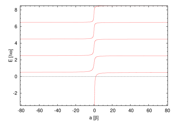
Figure 1: Energy spectrum for two particles in a harmonic trap as a function of the scattering length $a$ in units of the oscillator parameter $\beta$ according to [22].

The energy spectrum of the 2-body system in an isotropic harmonic trap is known exactly [22]. In Fig. 1, we show the energy spectrum as a function of the scattering length $a$ in free space measured in units of the oscillator length $\beta=\sqrt{\hbar/(m\omega)}$. In the unitary limit, the ground state energy approaches $\hbar\omega/2$.

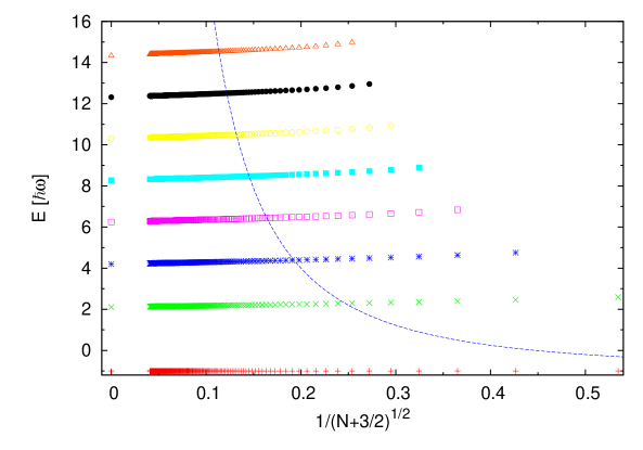
Figure 2: Energy spectrum for two particles in a harmonic trap as a function of the cutoff $N$ and exact results from [22] at $N\rightarrow\infty$ for $E_{0}=-\hbar\omega$. The dashed line indicates the value of the cutoff $N$ at which $N\approx 5E/(\hbar\omega)$.

We compare our numerical results to the exact solution in order to test the accuracy of our method. In Fig. 2, we show the results for the calculated spectra for $\epsilon^{\left(2\right)}=-1$ and cutoff parameters $N\leq 600$. The exact results [22] are added at $N\rightarrow\infty$. Already for finite values of the cutoff $N$ with $N\hbar\omega$ large compared to a calculated energy, we observe good agreement with the exact solution. The exact values can be reproduced numerically by extrapolating the results in the model spaces. We note, however, that this extrapolation is not strictly necessary if we interpret Eq. (2) as an effective Hamiltonian that is only accurate up to errors of order $\sqrt{E/(N\hbar\omega)}$. The dashed line indicates the value of the cutoff $N$ at which $N\approx 5E/(\hbar\omega)$. If this value of $N$ is reached, the effects from the finite cutoff are small and the extrapolation is usually not required. If more bodies are considered, however, it is computationally more expensive to go to large values of $N$ and extrapolation becomes necessary. In order to test the accuracy of our method, we have tried different extrapolations of our results for the 2-body energies and compared to the exact solution. The leading corrections from the finite cutoff $N$ scale as $1/\sqrt{N+3/2}$. A linear extrapolation of our results in $1/\sqrt{N+3/2}$ works very well. If only the points with $N>80$ are taken into account, linear and polynomial extrapolations give errors well below 1%.

2.2 Three and more bodies

In order to extend this procedure to the three and higher-body sector, two additional tools are needed: the Talmi-Moshinsky-Transformation (TMT) [39] and Wigner 6j symbols [40]. In the 3-body sector the finite model space is the linear hull of the tensor products $\phi_{n_{1}l_{1}m_{1}}\left(\vec{s}_{1}\right)\otimes\phi_{n_{2}l_{2}m_{2}}\left(\vec{s}_{2}\right)$ with the restriction $2\left(n_{1}+n_{2}\right)+l_{1}+l_{2}\leq N$. There are three 2-body contact interactions $V_{i}$ ($i=1,2,3$) and a 3-body contact interaction $V^{\left(3\right)}_{\textrm{cont}}$. The contributions of these interactions are most conveniently calculated in Jacobi coordinates $\vec{s}^{\left(i\right)}_{1}$ and $\vec{s}^{\left(i\right)}_{2}$, $i=1,2,3$). There are three different sets which are labelled by the coordinate $i$ not appearing in the definition of $\vec{s}^{\left(i\right)}_{1}$. The set $\vec{s}^{\left(3\right)}_{1}$, $\vec{s}^{\left(3\right)}_{2}$ is given by

$$\vec{s}^{\left(3\right)}_{1} =\frac{1}{\sqrt{2}}\left(\vec{x}_{1}-\vec{x}_{2}\right)\>,$$

$$\vec{s}^{\left(3\right)}_{2} =\frac{1}{\sqrt{6}}\left(\vec{x}_{1}+\vec{x}_{2}-2\vec{x}_{3}\right)\>,$$

and the other two combinations can be obtained by cyclically permuting the indices. In order to transform the matrix elements between different sets of coordinates the TMT is used. The Talmi-Transformation transforms a set of coordinates ($\rho$, $\lambda$) to a set ($\rho^{\prime}$, $\lambda^{\prime}$) via

$$\begin{pmatrix}\vec{\rho^{\prime}}\\ \vec{\lambda^{\prime}}\\ \end{pmatrix}=\underbrace{\begin{pmatrix}\sqrt{\frac{1}{1+d}}&-\sqrt{\frac{d}{1+d}}\\ \sqrt{\frac{d}{1+d}}&\sqrt{\frac{1}{1+d}}\\ \end{pmatrix}}_{M}\cdot\begin{pmatrix}\vec{\rho}\\ \vec{\lambda}\\ \end{pmatrix}\>,$$

where $d\geq 0$ is a real number. In our case, we need the transformation from one set of Jacobi coordinates to another set of Jacobi coordinates. The Talmi transformation with $d=3$ transforms the set ($\vec{s}^{\left(3\right)}_{1}$, $\vec{s}^{\left(3\right)}_{2}$) to the set ($-\vec{s}^{\left(1\right)}_{1}$, $-\vec{s}^{\left(1\right)}_{2}$) and the set ($\vec{s}^{\left(3\right)}_{1}$, $-\vec{s}^{\left(3\right)}_{2}$) to the set ($-\vec{s}^{\left(2\right)}_{1}$, $\vec{s}^{\left(2\right)}_{2}$), respectively. The corresponding expansion of the coupled oscillator functions depending on one set of Jacobi coordinates in oscillator functions depending on another set terminates after a finite number of terms, since the total oscillator energy, the total angular momentum, and the parity are conserved:

$$\left[\phi_{n_{\vec{\rho}}l_{\vec{\rho}}}\left(\vec{\rho}\right)\otimes\phi_{n_{\vec{\lambda}}l_{\vec{\lambda}}}\left(\vec{\lambda}\right)\right]^{L}_{M_{L}}=\sum\limits_{n^{\prime}_{\rho^{\prime}}l^{\prime}_{\rho^{\prime}}n^{\prime}_{\lambda^{\prime}}l^{\prime}_{\lambda^{\prime}}}\left<n^{\prime}_{\rho^{\prime}}l^{\prime}_{\rho^{\prime}},n^{\prime}_{\lambda^{\prime}}l^{\prime}_{\lambda^{\prime}};L|n_{\rho}l_{\rho},n_{\lambda}l_{\lambda}\right>_{d}\\ \left[\phi^{\beta}_{n^{\prime}_{\vec{\rho}\,^{\prime}}l^{\prime}_{\vec{\rho}\,^{\prime}}}\left(\vec{\rho}\,^{\prime}\right)\otimes\phi^{\beta}_{n^{\prime}_{\vec{\lambda}^{\prime}}l^{\prime}_{\vec{\lambda}^{\prime}}}\left(\vec{\lambda}^{\prime}\right)\right]^{L}_{M_{L}}\>.$$

The expansion coefficients $\left<n^{\prime}_{\rho^{\prime}}l^{\prime}_{\rho^{\prime}},n^{\prime}_{\lambda^{\prime}}l^{\prime}_{\lambda^{\prime}};L|n_{\rho}l_{\rho},n_{\lambda}l_{\lambda}\right>_{d}$ are the Brody-Moshinsky-Brackets.

The coupling constants of the 2-body interactions are determined by Eq. (4) for a given 2-body energy. The coupling constant $v^{\left(3\right)}$ of $V^{\left(3\right)}_{\textrm{cont}}$ is determined so that a given 3-body energy $\epsilon^{\left(3\right)}$ is reproduced. Using the separability of $V^{\left(3\right)}_{\textrm{cont}}$ one finds for the running coupling constant $v^{\left(3\right)}(N)$:

$$-\frac{\hbar\omega\pi^{3}}{v^{\left(3\right)}}=\sum_{k}\frac{\bigl{|}\sum\limits_{n_{\vec{s}_{1}},n_{\vec{s}_{2}}}Z\left(k;n_{\vec{s}_{1}}0,n_{\vec{s}_{2}}0,0\right)f_{n_{\vec{s}_{1}}}f_{n_{\vec{s}_{2}}}\bigr{|}^{2}}{D\left(k\right)-\epsilon^{\left(3\right)}}$$ (5)

with the eigenvector

$$\left|k\right>=\sum\limits_{n^{\prime}_{\vec{s}_{1}}l^{\prime}_{\vec{s}_{1}},n^{\prime}_{\vec{s}_{2}}l^{\prime}_{\vec{s}_{2}},L}^{N}Z\left(k;n^{\prime}_{\vec{s}_{1}}l^{\prime}_{\vec{s}_{1}},n^{\prime}_{\vec{s}_{2}}l^{\prime}_{\vec{s}_{2}},L\right)\left|n^{\prime}_{\vec{s}_{1}}l^{\prime}_{\vec{s}_{1}},n^{\prime}_{\vec{s}_{2}}l^{\prime}_{\vec{s}_{2}},L\right>\>,$$ (6)

corresponding to the eigenvalue problem $D(k)\left|k\right>=\left(\frac{H^{\left(2\right)}_{\textrm{osc}}+V_{1}+V_{2}+V_{3}}{\hbar\omega}\right)\left|k\right>$.

Analogous to the 3-body sector, the model space for four bodies is the linear hull of tensor products of HOF with $2\left(n_{1}+n_{2}+n_{3}\right)+l_{1}+l_{2}+l_{3}\leq N$. In order to determine all contributions of the interactions in one set of Jacobi-coordinates, the TMT is used again. The transformation is defined for coupled wave functions

$$\left[\left[\phi_{n_{1}l_{1}}\left(\vec{s}_{1}\right)\otimes\phi_{n_{2}l_{2}}\left(\vec{s}_{2}\right)\right]^{L_{12}}\otimes\phi_{n_{3}l_{3}}\left(\vec{s}_{3}\right)\right]^{L}_{M}\>.$$

For the TMT related to the mapping $\{\vec{s}_{2},\vec{s}_{3}\}\rightarrow\{\vec{s^{\prime}}_{2},\vec{s^{\prime}}_{3}\}$, the wave functions must at first be recoupled to

$$\left[\phi_{n_{1}l_{1}}\left(\vec{s}_{1}\right)\otimes\left[\phi_{n_{2}l_{2}}\left(\vec{s}_{2}\right)\otimes\phi_{n_{3}l_{3}}\left(\vec{s}_{3}\right)\right]^{L_{23}}\right]^{L^{\prime}}_{M^{\prime}}\>.$$

The overlap between these wave functions is given by the 6j symbols [40].

$$\bigl{<}\left[\left[\phi_{n_{1}l_{1}}\otimes\phi_{n_{2}l_{2}}\right]^{L_{12}}\otimes\phi_{n_{3}l_{3}}\right]^{L}_{M}\bigr{|}\left[\phi_{n_{1}l_{1}}\otimes\left[\phi_{n_{2}l_{2}}\otimes\phi_{n_{3}l_{3}}\right]^{L_{23}}\right]^{L^{\prime}}_{M^{\prime}}\bigr{>}=\\ \delta_{L,L^{\prime}}\delta_{M,M^{\prime}}\left(-1\right)^{l_{1}+l_{2}+l_{3}+L}\sqrt{\left(2L_{12}+1\right)\left(2L_{23}+1\right)}\begin{Bmatrix}l_{1}&l_{2}&L_{12}\\ l_{3}&L&L_{23}\end{Bmatrix}\>.$$

This construction of the model space can be generalised to $n$ bodies in a straightforward way.

3 Results for the 3-body sector

3.1 Unitary limit

We are now in the position to apply this effective theory to the 3- and 4-body sector. First, we focus on the 3-body sector in the unitary limit in order to test our method against the exact analytical solution [25]. The corresponding ground state energy for the 2-body system is $\epsilon^{\left(2\right)}=1/2$ [22]. Since the three coupling constants $v^{\left(2\right)}_{i}$ are identical, the Hamiltonian is invariant under permutation of the bodies. It follows that the Hamilton matrix is block diagonal in different symmetries of the wave functions. Typical values of the cutoff $N$ reached in our study for the 3-body problem are $N\approx 40...70$.

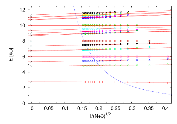
Figure 3: Energy spectrum for mixed antisymmetric states of three particles in a harmonic trap with $L^{P}=1^{-}$ as a function of $N$ and exact analytical results from [25]. The solid lines indicate the linear extrapolation to $N=\infty$ while the dashed line indicates the value of the cutoff $N$ at which $N\approx 5E/(\hbar\omega)$.

For mixed antisymmetric states, which are antisymmetric under exchange of the first two particles, $V^{\left(3\right)}_{\textrm{cont}}$ does not contribute. As an example, Fig. 3 presents the spectrum of states with angular momentum and parity $L^{P}=1^{-}$ depending on the cutoff $N$ in the unitary limit. Again, the exact results are added at $N\rightarrow\infty$. The dashed line indicates the value of the cutoff $N$ at which $N\approx 5E/(\hbar\omega)$. It is clear that for the higher excited states an extrapolation in $N$ is required. The spectrum can be extrapolated linearly in $1/\sqrt{N+3}$ as indicated by the solid lines.

For completely symmetric wave functions, however, the 3-body interaction $V^{\left(3\right)}_{\textrm{cont}}$ does contribute. Such wave functions can occur for systems of three identical bosons or three distinguishable particles which both display the Efimov effect. In Fig. 4, we show the spectrum for positive parity and $L=0$ as a function of the cutoff $N$. As a typical example, the 3-body interaction was adjusted such that the 3-body ground state has energy $E_{0}^{(3)}\equiv\epsilon^{\left(3\right)}\hbar\omega=-\hbar\omega$. In principle, any value could be taken for $\epsilon^{(3)}$. However, the renormalization energies $\epsilon^{(3)}$ and $\epsilon^{(2)}$ should be well within the energy range given by the finite cutoff $N$ in order to avoid large errors from the finite cutoff. As shown by Werner and Castin [25], there are two different types of states. On the one hand, there are states independent of $V^{\left(3\right)}$ (crosses). On the other hand, there are states which depend on $V^{\left(3\right)}$ (squares) and are called Efimov-like. These Efimov-like states are the analog of Efimov states in the trap. The exact results [25] are given at $N\rightarrow\infty$. The dashed line indicates the value of the cutoff $N$ at which $N\approx 5E/(\hbar\omega)$. Again, for the higher excited states an extrapolation is required. For the non-Efimov-like states a linear extrapolation is appropriate. The Efimov-like states, however, show a curvature. In this case, a quadratic term has to be included in the extrapolation. Typical extrapolation errors for Efimov-like states are of order 2-3% and less than 1% for the other states.

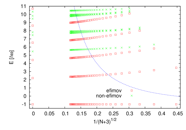
Figure 4: Energy spectrum for completely symmetric states of three particles in a harmonic trap with $L^{P}=0^{+}$ as a function of $N$ and exact analytical results from [25]. Efimov-like states are indicated by squares, other states are indicated by crosses. The dashed line indicates the value of the cutoff $N$ at which $N\approx 5E/(\hbar\omega)$.

3.2 Application to ⁶Li atoms

As an example application, we consider a system consisting of three fermionic ⁶Li atoms in a HOP with a low external magnetic field. Our calculations apply to experiments with a few fermions per site in optical lattices. The scattering lengths for the three lowest hyperfine states labelled by their hyperfine quantum numbers $|f,m_{f}\rangle$, or by integers: $|1\rangle=|1/2,+1/2\rangle$, $|2\rangle=|1/2,-1/2\rangle$ and $|3\rangle=|3/2,-3/2\rangle$ have been calculated by Julienne [41]. The Feshbach resonances occur for magnetic fields near $834$ G, $811$ G and $690$ G. The corresponding renormalisation energies are determined by the relation between the ground state energy $\epsilon^{\left(2\right)}$ and the scattering length $a$ in the 2 particle sector (See Fig.1). The range of interactions for ultracold atoms is the van der Waals length $l_{\textrm{vdW}}$, which is approximately $62.5\,a_{B}$ for ⁶Li, where $a_{B}=0.529\,$Å is the Bohr radius. Thus the effective theory is only reliable for regions, where $a\stackrel{{\scriptstyle>}}{{{}_{\sim}}}2l_{\textrm{vdW}}$. A discussion of Efimov physics in ⁶Li atoms with the three spin states $|1\rangle$, $|2\rangle$, and $|3\rangle$ without trap was given in Refs. [42, 43, 44, 45, 46]. As an example, we calculate the 3-body spectrum for the system $|1\rangle\otimes|1\rangle\otimes|2\rangle$ which contains two like atoms in the trap. Because of the Pauli principle, there are no Efimov-like states and $V^{\left(3\right)}_{\textrm{cont}}$ does not contribute. The energy spectrum of two-component fermions in a trap as a function of the scattering length $a$ was previously studied in Refs. [26, 27, 28, 29, 30, 31, 32, 33, 34, 35, 36]. Figure 5 shows the extrapolated energies of the first two states with $L^{P}=0^{+}$ as a function of the magnetic field (circles and pluses). The oscillator length is taken as $\beta\approx 65\,a_{B}$.

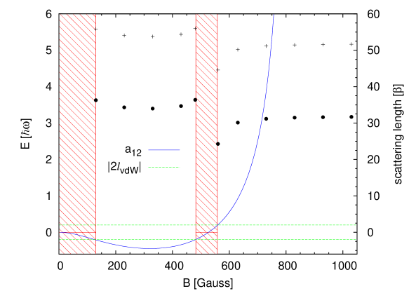
Figure 5: The energies of first two $0^{+}$ states in the 3-body system $|1\rangle\otimes|1\rangle\otimes|2\rangle$ indicated by circles and pluses (left scale) as function of the magnetic field. The solid and dashed lines give the scattering length $a_{12}$ from [41] and the van der Waals length $l_{\textrm{vdW}}$ (right scale).

The solid and dashed lines give the scattering length $a_{12}$ from [41] and the van der Waals length $l_{\textrm{vdW}}$ (right scale). The hatched areas indicate where the scattering length can not be considered large and our theory is not applicable. Outside of the hatched areas, our calculation should be accurate up to corrections of order $l_{\textrm{vdW}}/a_{12}$ and $l_{\textrm{vdW}}/\beta$. The magnetic field dependence of both states is very weak despite the strong variation of the scattering length $a_{12}$. The energies of the ground and first excited state are of order $3.2\hbar\omega$ and $5.2\hbar\omega$, respectively.

4 Results for the 4-body sector

We now turn to the 4-body system. We consider two types of 4-body systems both of which can display Efimov physics and focus on the systematics of the bound state spectrum. First, we consider two identical fermions with two other distinguishable particles. Because of the two identical fermions involved, this system is calculationally simpler than the 4-boson system which we calculate in the second step. Typical values of the cutoff $N$ reached in our study for the 4-body problem are $N\approx 20...30$.

4.1 Two identical fermions and two distinguishable particles

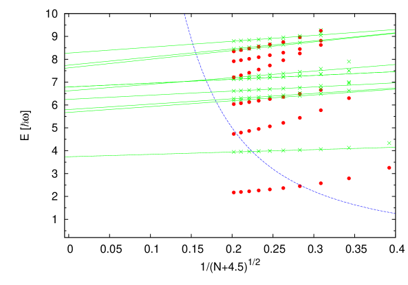
Figure 6: Energy spectrum for two identical fermions and two distinguishable particles with $L^{P}=0^{+}$ in a harmonic trap as a function of $N$. The system is in the unitary limit and $\epsilon^{\left(3\right)}=-0.5$. Efimov-like states are indicated by circles while universal states not sensitive to $\epsilon^{(3)}$ are given by crosses. The solid lines indicate the linear extrapolation to $N=\infty$ while the dashed line marks the value of the cutoff $N$ at which $N\approx 5E/(\hbar\omega)$.

We start with the case of two identical fermions with two other distinguishable particles. Thus, the wave function is antisymmetric under permutation of the identical fermions. Altogether, there are five 2-particle contact interactions and two 3-particle contact interactions. The contributions of some interactions are pairwise identical because two of the particles are identical. Analogous to the 3-body sector, the four coupling constants of the 2-particle interactions are renormalised by Eq. (4) and the two coupling constants of the 3-particle interactions by Eq. (5) for given ground state energies $\epsilon^{\left(2\right)}$ and $\epsilon^{\left(3\right)}$. We find both Efimov-like states which are sensitive to the value of $\epsilon^{\left(3\right)}$ and universal states which are independent of $\epsilon^{\left(3\right)}$. At higher energies, we also find non-interacting eigenstates which are not sensitive to both $\epsilon^{\left(2\right)}$ and $\epsilon^{\left(3\right)}$. As in the 2- and 3-body sector, the universal states can be extrapolated linearly while the Efimov-like states require a quadratic extrapolation. Here we require that no minimum exists for $1/N>0$ in order to get stable results. In Fig. 6, we show our results for the spectrum states with $L^{P}=0^{+}$ in the unitary limit and for $\epsilon^{\left(3\right)}=-0.5$. The dashed line indicates the value of the cutoff $N$ at which $N\approx 5E/(\hbar\omega)$. For all but the lowest two states the condition $N\stackrel{{\scriptstyle>}}{{{}_{\sim}}}5E/(\hbar\omega)$ is not satisfied for the values of $N$ reached in this calculation. As a consequence, a stable extrapolation for $N\to\infty$ is required to obtain reliable results. Since the exact results are not known, we estimate the uncertainty from the extrapolation conservatively as being equal to the energy shift from the last calculated value to the extrapolated value. This procedure should give an upper bound on the extrapolation uncertainty.

In order to understand the systematics of the trapped spectra, we investigate the 4-body spectrum as a function of the input parameters $\epsilon^{\left(2\right)}$ and $\epsilon^{\left(3\right)}$ analogous to the Efimov plot in free space [3]. In Fig. 7, the extrapolated spectra for two identical fermions with two other distinguishable particles in the unitary limit are shown for various ground state energies $\epsilon^{\left(3\right)}$ by the circles. Additionally, the exact results for the Efimov-like states in the 3-body sector are shown (squares). Both the 3- and the 4-body states depend on $\epsilon^{\left(3\right)}$ approximately linearly in this region but the slope of the 4-body states is typically larger.

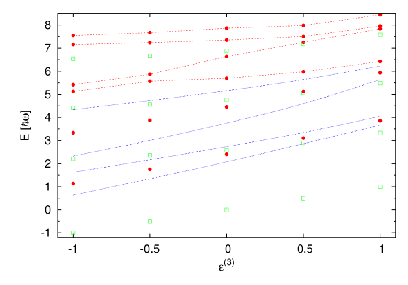
Figure 7: Extrapolated spectra for Efimov-like $0^{+}$ states in the 4-body sector of two identical fermions with two other distinguishable particles (circles) and in the 3-body sector (squares) for various $\epsilon^{\left(3\right)}$ in the unitary limit. The dotted lines give our upper bound on the extrapolation error for the two lowest states. The dashed lines are guides to the eye.

The dotted lines give our upper bound on the extrapolation error for the two lowest 4-body states. For the higher states the extrapolation error is similar. The higher excited states are connected by dashed lines to guide the eye. Note that the 4-body ground state is above the 3-body ground state in this case. Around $\epsilon^{\left(3\right)}\approx 0.25$, the trajectories of lowest two and of the 4th 4-body state cross the next higher 3-body state. In free space, the corresponding 4-body state would become unstable to decay into the trimer and another particle, but in the trap this behavior can in principle be observed experimentally. The other 4-body states are different in nature and move parallel with the nearest 3-body state and never cross.

4.2 Four identical bosons

We now turn to the system of four identical bosons with $L^{P}=0^{+}$. This system is of high experimental interest and the behavior of the states in free space is well known [16, 17]. Figure 8 shows the calculated spectrum in the unitary limit as a function of $N$ for $\epsilon^{\left(3\right)}=-1$.

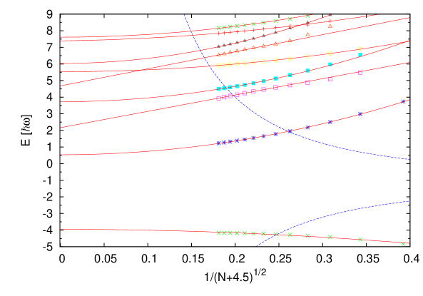
Figure 8: Spectrum for symmetric $0^{+}$ states of four identical bosons in the unitary limit for $\epsilon^{\left(3\right)}=-1$ as a function of $N$. The solid lines indicate the extrapolation to $N=\infty$ while the dashed line indicates the value of the cutoff $N$ at which $N\approx 5E/(\hbar\omega)$.

The dashed line indicates the value of the cutoff $N$ at which $N\approx 5E/(\hbar\omega)$. For most of the states, the condition $N\stackrel{{\scriptstyle>}}{{{}_{\sim}}}5E/(\hbar\omega)$ is not satisfied and we therefore have to rely on the extrapolation. Again, we find both Efimov-like states which are sensitive to the value of $\epsilon^{\left(3\right)}$ and universal states which are independent of $\epsilon^{\left(3\right)}$. At higher energies, we also find non-interacting eigenstates which are insensitive to both $\epsilon^{\left(2\right)}$ and $\epsilon^{\left(3\right)}$. In the following, we focus on the Efimov-like states. They are extrapolated with a quadratic polynomial. Some of the extrapolations are shown by the solid lines in Fig. 8. Again, we estimate the uncertainty from the extrapolation conservatively as being equal to the energy shift from the last calculated value to the extrapolated value.

We are now in the position to study the structure of the 3- and 4-body spectra for the Efimov-like states. In the original Efimov plot, the 3-body spectrum is studied for fixed 3-body interaction $V^{\left(3\right)}$ while the 2-body energy is varied [1, 3]. Since there is no 4-body interaction at leading order, this plot can be extended to the 4-body system and has been studied extensively in free space [16, 17]. We will compare our spectra with the free space results. In Fig. 9, the extrapolated spectra of the symmetric $0^{+}$ 4-body states for various $\epsilon^{\left(2\right)}$ are shown by the circles. The 3-body interaction is fixed by the requirement, that the 3-body ground state lies at $\epsilon^{\left(3\right)}=-1$ in the unitary limit. Additionally, the 3-body Efimov-like states are shown as squares.

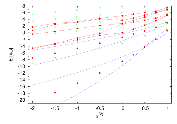
Figure 9: Extrapolated spectra of the symmetric 4-body states $0^{+}$ for various $\epsilon^{\left(2\right)}$ (circles) and 3-body Efimov-like states (squares). The 3-body interaction is fixed such that $\epsilon^{\left(3\right)}=-1$ in the unitary limit. The dotted lines give our upper bound on the extrapolation error for the two lowest states. The dashed lines are guides to the eye.

As before, the dotted lines give our upper bound on the extrapolation error for the two lowest 4-body states. The higher excited states are connected by dashed lines to guide the eye. Their extrapolation error is similar but not shown explicitly. The harmonic confinement has a strong effect on the spectrum. Compared to free space, it is no longer true that two 4-body states are attached to each trimer state. Moreover, the levels appear to interact strongly. There are various avoided crossings of 4-body states, e.g. between the 4th and 5th state around $\epsilon^{\left(2\right)}\approx 0$ and possibly also between the second and third state. These avoided crossings could be studied experimentally by varying $\epsilon^{\left(2\right)}$ using Feshbach resonances.

The dependence on $\epsilon^{\left(2\right)}$ can be translated into a dependence on the scattering length $a$ using Fig. 1. For $\epsilon^{\left(2\right)}$ between minus two and zero, the scattering length is essentially zero. When $\epsilon^{\left(2\right)}$ is varied from zero to one, however, the scattering length grows to become infinite at $\epsilon^{\left(2\right)}=1/2$, jumps to minus infinity and approaches a negative value close to zero at $\epsilon^{\left(2\right)}=1$. This is the most interesting region from the point of universality and corresponds to the usual Efimov plot in free space. In this region, the scattering length is much larger than all other length scales and our effective theory is expected to describe systems of real atoms with van der Waals interactions. The discrete scale invariance of the 3- and 4-body spectra in free space has disappeared in Fig. 9. It would be interesting to approach the free space limit by making the trap wider and wider but keeping the scattering length $a$ and the 3-body interaction fixed. This corresponds to looking at the same physical system in a wider trap in order to see how the discrete scaling symmetry is restored. In the theoretical calculation, taking this limit is computationally very expensive since the absolute value of the energy cutoff for fixed $N$ vanishes as $\beta\to\infty$. Cold atom experiments could serve as a quantum simulator to study this question.

In Fig. 10, we show a different variant of this plot. The extrapolated spectra for 4-body $0^{+}$ states are given for various 2-body energies $\epsilon^{\left(2\right)}$ (circles). The 3-body interaction is renormalised with the requirement, that the 3-body ground state energy lies at $\epsilon^{\left(3\right)}=-1$ for each chosen $\epsilon^{\left(2\right)}$. Further, the Efimov-like 3-body states are added as squares.

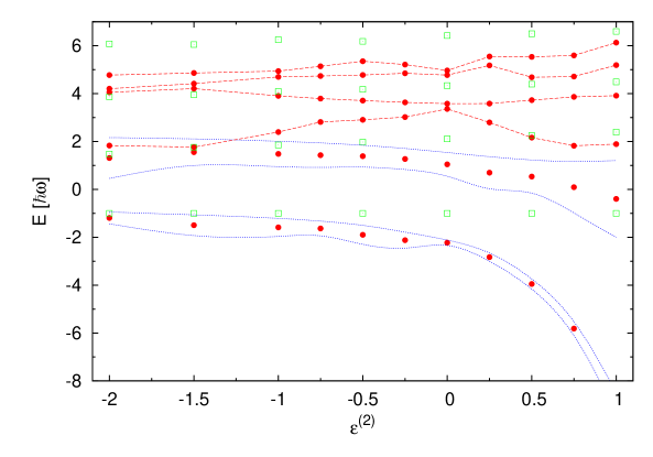
Figure 10: Extrapolated spectra of the symmetric 4-body (circles) and 3-body Efimov-like (squares) states $0^{+}$ for various $\epsilon^{\left(2\right)}$. For each $\epsilon^{\left(2\right)}$ the 3-body interaction is renormalised with the requirement, that the 3-body ground state lies at $\epsilon^{\left(3\right)}=-1$. The dotted lines give our upper bound on the extrapolation error for the two lowest states. The dashed lines are guides to the eye.

The extrapolation error estimates for the lowest two states are again given by the dotted lines. There are also avoided crossings for the higher states near $\epsilon^{\left(2\right)}\approx 0$. In general, the spectrum is very different since the 3-body ground state is forced to be at $\epsilon^{\left(3\right)}=-1$. Experimentally, this situation is currently not accessible. It would require a second “3-body” Feshbach resonance that can be used to keep the 3-body ground state energy constant.

5 Summary and Conclusions

In this work, we have studied the universal properties of few-body systems with large scattering length in a harmonic trap. We have used an effective theory for short-range interactions and identified the cutoff on the harmonic oscillator basis functions with the cutoff of the effective theory [37]. The effective theory is then formulated directly in the model space and the low-energy constants are fixed by matching to few-body observables in the trap. The few-body states in the trap are then obtained by diagonalization of the finite Hamiltonian matrix. After renormalization, the spectrum is independent of the cutoff up to small corrections. If the cutoff can not be taken sufficiently large, it is possible to extrapolate to larger values.

Our work has focused on systems where the Efimov effect occurs. In this case, a 3-body interaction already enters at leading order and the corresponding low-energy constant has to be fixed by a 3-body observable. We have checked our numerical method against exact analytical results for the 3-body system in the unitary limit and found good agreement. Using the magnetic field dependence of the ⁶Li scattering lengths calculated by Julienne [41], we have predicted the lowest two states in a two-state mixture as an example.

The main part of the work focused on the 4-body system in a harmonic trap. We considered two types of 4-body systems both of which can display Efimov physics. First, we considered two identical fermions with two other distinguishable particles. Second, we calculated the spectrum for four identical bosons. In both cases, we found both Efimov-like states which are sensitive to the value of $\epsilon^{\left(3\right)}$ and universal states which are independent of $\epsilon^{\left(3\right)}$. At higher energies, there are also non-interacting eigenstates which are insensitive to both $\epsilon^{\left(2\right)}$ and $\epsilon^{\left(3\right)}$. We found a number of interesting features in the spectra, such as avoided crossings of 4-body states and 4-body states crossing 3-body states if the 2- or 3-body energies are increased. It would be very interesting to observe these features experimentally. The trap introduces the oscillator length $\beta$ as a new scale and breaks the discrete scaling symmetry from free space. In the calculated spectra no remnants of the discrete scaling symmetry were observed.

The extrapolation error of the calculated energies has been estimated conservatively from the difference of the last calculated value and the extrapolated value of the energy. These errors could be improved by going to larger values of $N$. However, it would also be desirable to understand the leading corrections from the finite model space in more detail. Similar studies in free space have been carried out [47].

In general, the trap has a strong influence on the overall structure of the spectrum. In particular, the discrete scaling symmetry and the connection of two 4-body states to each trimer state known from free space could not be observed. In the future it would be interesting to understand this modification in more detail by varying the size of the trap. Moreover, the extension to more bodies would allow to study the transition from few- to many-body systems. While this is in principle straightforward, the computational effort grows substantially.

References

- [1] E. Braaten and H.-W. Hammer, Phys. Rept. 428, 259 (2006).
- [2] H.-W. Hammer and L. Platter, Ann. Rev. Nucl. Part. Sci. 60, 207 (2010).
- [3] V. Efimov, Phys. Lett. 33B, 563 (1970).
- [4] V. Efimov, Sov. J. Nucl. Phys. 29, 546 (1979).
- [5] P.F. Bedaque, H.-W. Hammer, and U. van Kolck, Phys. Rev. Lett. 82, 463 (1999). Nucl. Phys. A 646, 444 (1999).
- [6] T. Kraemer, M. Mark, P. Waldburger, J.G. Danzl, C. Chin, B. Engeser, A.D. Lange, K. Pilch, A. Jaakkola, H.-C. Nägerl, and R. Grimm, Nature 440, 315 (2006).
- [7] T. B. Ottenstein, T. Lompe, M. Kohnen, A. N. Wenz, S. Jochim, Phys. Rev. Lett. 101, 203202 (2008).
- [8] J. H. Huckans, J. R. Williams, E. L. Hazlett, R. W. Stites, K. M. O’Hara, Phys. Rev. Lett. 102, 165302 (2009).
- [9] G. Barontini, C. Weber, F. Rabatti, J. Catani, G. Thalhammer, M. Inguscio, F. Minardi, Phys. Rev. Lett. 103, 043201 (2009).
- [10] N. Gross, Z. Shotan, S. Kokkelmans, L. Khaykovich, Phys. Rev. Lett. 103, 163202 (2009).
- [11] M. Zaccanti, B. Deissler, C. D’Errico, M. Fattori, M. Jona-Lasinio, S. Müller, G. Roati, M. Inguscio, G. Modugno, Nature Physics 5, 586 (2009).
- [12] S. Knoop, F. Ferlaino, M. Mark, M. Berninger, H. Schoebel, H.-C. Naegerl, R. Grimm, Nature Physics 5, 227 (2009).
- [13] T. Lompe, T. B. Ottenstein, F. Serwane, K. Viering, A. N. Wenz, G. Zürn, S. Jochim, Phys. Rev. Lett. 105, 103201 (2010).
- [14] S. Nakajima, M. Horikoshi, T. Mukaiyama, P. Naidon and M. Ueda, Phys. Rev. Lett. 105, 023201 (2010).
- [15] T. Lompe, T.B. Ottenstein, F. Serwane, A.N. Wenz, G. Zürn, S. Jochim, arXiv:1006.2241 [cond-mat.quant-gas].
- [16] H.-W. Hammer and L. Platter, Eur. Phys. J. A 32, 113 (2007).
- [17] J. von Stecher, J. P. D’Incao, and C. H. Greene, Nature Physics 5, 417 (2009).
- [18] A. Deltuva, arXiv:1009.1295 [physics.atm-clus].
- [19] F. Ferlaino, S. Knoop, M. Berninger, W. Harm, J. P. D’Incao, H.-C. Nägerl, R. Grimm, Phys. Rev. Lett. 102, 140401 (2009).
- [20] S. Pollack, D. Dries, and R. Hulet, Science 326, 1683 (2009).
- [21] J. von Stecher, J. Phys. B: At. Mol. Opt. Phys. 43, 101002 (2010).
- [22] T. Busch, B.-G. Englert, K. Rzazewski and M. Wilkens, Found. Phys. 28, 549 (1998).
- [23] S. Jonsell, H. Heiselberg and C. J. Pethick, Phys. Rev. Lett. 89, 250401 (2002).
- [24] S. Tan, arXiv:cond-mat/0412764.
- [25] F. Werner and Y. Castin, Phys. Rev. Lett. 97, 150401 (2006).
- [26] S.Y. Chang and G.F. Bertsch, Phys. Rev. A 76, 021603 (2007).
- [27] J. von Stecher and C.H. Greene, Phys. Rev. Lett. 99, 090402 (2007).
- [28] D. Blume, J. von Stecher, and C.H. Greene, Phys. Rev. Lett. 99, 233201 (2007).
- [29] I. Stetcu, B. R. Barrett, U. van Kolck and J. P. Vary, Phys. Rev. A 76, 063613 (2007).
- [30] J.P. Kestner and L.-M. Duan, Phys. Rev. A 76, 033611 (2007).
- [31] T. Luu and A. Schwenk, Phys. Rev. Lett. 98, 103202 (2007).
- [32] J. von Stecher, C.H. Greene and D. Blume, Phys. Rev. A 77, 043619 (2008).
- [33] Y. Alhassid, G.F. Bertsch, and L. Fang, Phys. Rev. Lett. 100, 230401 (2008).
- [34] I. Stetcu, J. Rotureau, B. R. Barrett and U. van Kolck, Ann. Phys. 325, 1644 (2010).
- [35] J. Rotureau, I. Stetcu, B. R. Barrett, M. C. Birse and U. van Kolck, arXiv:1006.3820 [cond-mat.quant-gas].
- [36] X.-J. Liu, H. Hu, P.D. Drummond, Phys. Rev. A 82, 023619 (2010).
- [37] I. Stetcu, B. R. Barrett and U. van Kolck, Phys. Lett. B 653, 358 (2007).
- [38] S. Tölle, H.-W. Hammer and B.C. Metsch, EPJ Web of Conferences 3, 02004 (2010).
- [39] T. A. Brody, Tablas de Paréntesis de Transformación, Universidad Nacional Autonoma de Mexiko (1960).
- [40] D. A. Varshalovich, et al., Quantum Theory of Angular Momentum, 2nd Edition, World Scientific Publishing (1988).
- [41] P.S. Julienne, private communication.
- [42] E. Braaten, H.-W. Hammer, D. Kang and L. Platter, Phys. Rev. A 81, 013605 (2010).
- [43] S. Nakajima, M. Horikoshi, T. Mukaiyama, P. Naidon and M. Ueda, Phys. Rev. Lett. 105, 023201 (2010).
- [44] E. Braaten, H.-W. Hammer, D. Kang and L. Platter, Phys. Rev. Lett. 103, 073202 (2009).
- [45] P. Naidon and M. Ueda, Phys. Rev. Lett. 103, 073203 (2009).
- [46] S. Floerchinger, R. Schmidt and C. Wetterich, Phys. Rev. A 79, 053633 (2009).
- [47] C. Ji, D. Phillips and L. Platter, Europhys. Lett. 92, 13003 (2010), and references therein.