Abundance analyses of helium-rich subluminous B stars

Abstract

The connection between helium-rich hot subdwarfs of spectral types O and B (He-sdB) has been relatively unexplored since the latter were found in significant numbers in the 1980’s. In order to explore this connection further, we have analysed the surface composition of six He-sdB stars, including LB 1766, LB 3229, SB 21 (= Ton-S 137 = BPS 29503-0009), BPS 22940–0009, BPS 29496–0010, and BPS 22956–0094. Opacity-sampled line-blanketed model atmospheres have been used to derive atmospheric properties and elemental abundances. All the stars are moderately metal-poor compared with the Sun ([Fe/H]$\approx-0.5$). Four stars are nitrogen-rich, two of these are carbon-rich, and at least four appear to be neon-rich. The data are insufficient to rule out binarity in any of the sample. The surface composition and locus of the N-rich He-sdBs are currently best explained by the merger of two helium white dwarfs, or possibly by the merger of a helium white dwarf with a post-sdB white dwarf. C-rich He-sdBs require further investigation.

1 Introduction

Subdwarf B stars are low-mass core-helium burning stars with extremely thin hydrogen envelopes. They behave as helium main-sequence stars of roughly half a solar mass. Their atmospheres are generally helium deficient; radiative levitation and gravitational settling combine to make helium sink below the hydrogen-rich surface (Heber, 1986).

However, almost 5$\%$ of the total subdwarf population comprise stars with helium-rich atmospheres (Green et al., 1986; Ahmad & Jeffery, 2006). The optical spectra of these stars are characterised by strong neutral helium lines and weak Heii lines; they exhibit a wide range of helium abundance and effective temperatures ($T_{\rm eff}$) similar to both sdB and sdO stars. They have been variously classified as sdOB, sdOC and sdOD (Green et al., 1986) stars, but more recently as He-sdB and He-sdO stars (Moehler et al., 1990; Ahmad & Jeffery, 2004). The spectroscopic division concerns the relative strengths of Hei 4471, Heii 4541 and H$\gamma$ (itself a blend of H and Heii). Roughly speaking, the division occurs for stars with $T_{\rm eff}\approx 38\,000\,{\rm K}$ Drilling et al. (2003).

In general, He-sdB stars have lower surface gravities ($g$) than normal hydrogen-rich sdB stars (Heber, 2009) and have spectral characteristics intermediate between extreme helium (EHe) stars (Jeffery, 1996) and He-sdO stars (Napiwotzki, 2008).

Most He-sdB stars show strong nitrogen (Nii and Niii) lines in their optical spectrum; these are referred to as N-rich by Drilling et al. (2003). A few also showing strong carbon (Cii and Ciii) lines are labelled C-rich.

The question posed by these stars is that of their evolutionary status. Do He-sdB and He-sdO stars form a single sequence? Why are there C-rich and N-rich stars? Why is there such a large range in hydrogen abundance? How are they related to other classes of evolved star, including normal sdB stars? Is there a connection with any of the extreme helium stars (Jeffery, 2008a, b)?

Possible origins include: a late core flash of a single post-giant-branch helium star evolving toward the white dwarf sequence (Lanz et al., 2004; Miller Bertolami et al., 2008); the merger of two helium white dwarfs (Iben, 1990; Saio & Jeffery, 2000); and the merger of a helium white dwarf with a post-sdB star (Justham et al., 2010). All of these scenarios are likely to produce hot subdwarfs with He-rich and N-rich surfaces. The second has also been argued to lead to helium-poor “normal” sdB stars. All predict evolution tracks that commence with shell helium-ignition in a white dwarf. They take the star to a yellow-giant on a thermal time-scale and then to the helium main-sequence on a nuclear timescale. The details of the tracks differ in respect of their initial conditions and the micro-physics adopted. Whether carbon is exposed is not clear.

The goal is, if possible, to distinguish clearly the various types of observed He-sdB (and He-sdO) stars and to connect each to one of these diverse origins.

The surface abundances of elements other than hydrogen and helium are therefore important indicators of previous evolution. But first it is necessary to establish in what ranges these abundances lie, and hence to identify whether distinct groups exist. The challenge is that the numbers of He-sdB and He-sdO stars bright enough for fine analysis has hitherto been small, and very few, so far, have been found to be spectroscopically similar. The first of our studies was of PG1544+488, which surprisingly turned out to be a short-period binary containing two helium-rich sdB stars (Ahmad & Jeffery, 2004). The second was for JL 87 (Ahmad et al., 2007), a relatively bright and only moderately helium-rich ($n_{\rm He}/n_{\rm H}\approx 0.4$) and carbon-rich subdwarf. Far-ultraviolet spectra of these, and of LB 1766, were previously analyzed by Lanz et al. (2004), with quite different results to our own. Ahmad et al. (2007) demonstrated the importance of establishing $T_{\rm eff}$, $\log g$ and carbon abundances from optical spectra of Hei lines, i.e. relatively unblended lines with well-understood broadening theory, before extracting abundances of subordinate species.

We are therefore systematically acquiring high-resolution high signal-to-noise optical spectroscopy of He-sdB stars. § 2 describes the observations used in this paper. These data are used to carry out detailed abundance analyses, making use of the latest generation of fully line-blanketed model atmospheres for appropriate mixtures (§,3). § 4 presents the results for our programme stars, which are discussed in terms of the evolution models and analyses of related objects in § 5.

Table 1: AAT/UCLES Observing Log

Star		$\alpha\leavevmode\nobreak\ \leavevmode\nobreak\ \leavevmode\nobreak\ (2000)\leavevmode\nobreak\ \leavevmode\nobreak\ \leavevmode\nobreak\ \delta$		$m_{\rm V}$
UT (Start)	Seeing	$t_{\rm exp}$ (s)	S/N
BPS CS 22940–0009		20 30 20	–59 50 50	13.8
2005 08 26 09:25:40	1.4”	1800	10
2005 08 26 09:56:33	1.4”	1800	10
2005 08 26 10:27:29	1.4”	1800	12
2005 08 26 10:58:22	1.4”	1800	10
Mean			21
LB 1766		04 59 19	–53 52 52	12.3
2005 08 26 17:22:30	2.0”	1800	35
2005 08 26 17:53:23	2.0”	1800	35
2005 08 29 16:00:55	1.7”	1800	20
2005 08 29 16:31:49	1.7”	1800	20
Mean			61
BPS CS 22956–0094		22 16 56	–64 31 51	–
2005 08 27 11:42:19	1.5”	1800	17
2005 08 27 12:13:13	1.5”	1800	13
2005 08 27 12:44:07	1.5”	1800	20
Mean			28
BPS CS 29496–0010		23 34 02	–28 51 38	14.7
2005 08 27 14:07:52	1.8”	1800	10
2005 08 27 14:38:46	1.8”	1800	10
2005 08 27 15:09:40	1.8”	1800	10
2005 08 27 15:40:37	1.5”	1800	10
2005 08 27 16:21:17	1.5”	1800	10
2005 08 27 16:52:10	1.5”	1800	10
2005 08 27 17:23:04	1.5”	1800	10
2005 08 27 17:54:36	1.5”	1800	10
Mean			25
LB 3229 = JL 261		01 47 17	–51 33 39	13.6
2005 08 27 18:29:28	1.5”	1800	17
2005 08 27 19:00:23	1.5”	1800	18
Mean			25
SB 21 = PHL 645 = Ton-S 137 = BPS CS 29503–0009
		00 04 31	–24 26 18	13.9
2005 08 28 14:46:45	1.2”	1800	20
2005 08 28 15:17:39	1.2”	1800	20
2005 08 28 15:48:33	1.2”	1800	20
2005 08 28 16:19:27	1.2”	1800	19
2005 08 28 16:50:21	1.2”	1800	18
2005 08 28 17:21:15	1.2”	1800	18
2005 08 28 17:52:09	1.2”	1800	15
2005 08 28 18:24:53	1.4”	1800	17
Mean			52

2 Observations

Spectra of several hydrogen-deficient stars were obtained with the University College London Echelle Spectrograph on the Anglo-Australian Telescope (AAT) in August 2005. These included a number of He-sdB stars, namely LB 1766, LB 3229, SB 21 (= Ton-S 137 = BPS 29503-0009), BPS 22940–0009, BPS 29496–0010, and BPS 22956–0094. An extract from the observing log is shown in Table 1, which also indicate the signal-to-noise ratio of the combined spectra used here. UCLES was configured with the 31.6 lines mm^-1 grating, the EEV2 detector, and a slit width of 1.09 mm. A central wavelength of 4340.02 Å gives complete spectral coverage between 3820 and 5200 Å, and a nominal resolution with this slit width $R\approx 32\,000$. Exposures were broken into 1800 s segments in order to minimise cosmic-ray contamination.

A preliminary analysis of three of these stars (LB 1766, SB 21, and BPS 22940-0009) using the same data was given by (Naslim et al., 2010). SB 21 was originally identified as an extremely helium-rich subdwarf (Hunger & Kudritzki, 1980); Hunger et al. (1981) found this star to be comparable with the helium-rich hot subdwarfs, CPD$-31^{\circ}1701$ and TON-S 103. Abundances for LB 1766 were previously obtained from a far-ultraviolet (FUV) spectrum (Lanz et al., 2004); experience has demonstrated that an analysis of the FUV spectrum alone can lead to systematic errors (Ahmad et al., 2007). Our AAT spectra show LB 1766 and SB 21 to be nearly identical. Note that the original analyses (Lanz et al., 2004; Hunger & Kudritzki, 1980) suggest these two stars to be quite different; thus a detailed contemporary comparison is important.

BPS 22940–0009 and BPS 29496–0010 were identified as He-sdB stars and BPS 22956–0094 as an sdB star in the survey of Beers et al. (1992). Our spectra show BPS 22940–0009 and BPS 22956–0094 to be carbon-rich He-sdB stars with strong Cii, Ciii, Nii, Niii, and Hei lines. In contrast, LB 1766, SB 21, BPS 29496–0010 and LB 3229 are carbon poor He-sdB stars, but with strong Nii, Niii, and Hei lines.

The observations were reduced using a combination of ECHOMOP routines (Mills et al., 2006) and bespoke échelle reduction software (SŞahìn, 2008). The sky-subtracted wavelength-calibrated spectrum was extracted to a 2-d format with each order represented by a single row. Continuum normalization was achieved by smoothing the 2-d spectrum to form a 2-d envelope spectrum, and then dividing by said envelope to remove most of the échelle blaze function. The smoothing procedure was adjusted to ensure that strong lines (Balmer or Hei 4471 for example) were avoided when producing the normalisation function. Order merging was carried out using the same 2-d envelope to provide the weights at each wavelength in each overlap interval. A final normalisation step was carried out in which the merged 1-d spectrum was divided by a low-order polynomial fitted to a set of continuum points defined manually.

We found no radial velocity shifts amongst the repeat spectra of individual stars, but only the data for LB 1766 were spread over a significant time interval (3 days).

In order to obtain a spectrum with the highest possible signal-to-noise ratio, all of the individual spectra for each object were merged together, weighted appropriately for the signal-to-noise ratio in each spectrum. The combined spectra were velocity-shifted to the rest frame.

In an iterative process, we successfully identified all of the significant absorption lines visible in the combined spectra. Where observations allow (e.g. LB 1766 and SB 21), all known permitted and forbidden lines of Hei can be identified (cf. HD144941: Underhill, 1966; Harrison & Jeffery, 1997; Beauchamp & Wesemael, 1998). Heii4686 is present in all targets. Hydrogen Balmer lines are evident in BPS 22956–0094. Heii4541 and other Heii Pickering lines are present in LB 3229 and BPS 29496–0010. In the remainder, an H$\beta$/Heii4859 blend is present; it is not obvious from H$\gamma$ or Heii4541 which is dominant. In addition to Nii,iii, the target spectra variously show lines due to Cii,iii, Oii, Neii, Mgii, Aliii, Siiiii,iv and Siii. Identification charts are given in Figs. 6 – 11 (online only).

Figure 1: Theoretical model fits to Hei 4471 in LB 3229 for model atmospheres with $n_{\rm He}=0.989$, $T_{\rm eff}=40\,000\,{\rm K}$ and $\log g=4.0(0.5)6.0$.

Figure 2: The loci of ionization equilibria for Nii/Niii and Heii, the profile fits to Hei lines, and the adopted solution for LB 3229.

3 Physical parameters of He-sdBs

The goal was to measure atmospheric physical parameters $T_{\rm eff}$, $\log g$ and elemental abundances for each star. We adopted two methods to determine $T_{\rm eff}$ and $\log g$. In the first we used ionisation equilibria of prominent ions to determine $T_{\rm eff}$ and the profiles of Stark-broadened Hei lines to determine $\log g$. In the second we used the $\chi^{2}$-minimization package SFIT (Ahmad & Jeffery, 2003) to determine $T_{\rm eff}$ and $\log g$ simultaneously.

3.1 Model atmospheres, line formation and spectral synthesis

Grids of model atmospheres for hydrogen-deficient stars were calculated using the LTE line-blanketed code STERNE (Behara & Jeffery, 2006) which uses Opacity Project data for the continuous opacities, and treats line-blanketing through opacity sampling in a database of some $10^{8}$ atomic transitions. In this case, we adopted grids with 1/10 solar metallicity, relative helium abundances $n_{\rm He}=0.50$, 0.70, 0.90, 0.95, 0.989 and 0.999 by number, and assumed micro-turbulent velocities $v_{\rm t}=5$ and $10\,{\rm km\,s^{-1}}$.

The choice of the 1/10 solar metallicity grid was adopted primarily because we were unable to obtain satisfactory fits for solar abundance models. The average abundances of Si and Mg, which are unlikely to have been affected by evolution, are sub-solar by $\approx 0.5$ dex (see below).

Given a model atmosphere, the LTE radiative-transfer code SPECTRUM (Jeffery et al., 2001) may be used to compute a) individual line profiles and equivalent widths for given abundances and $v_{\rm t}$, b) synthetic spectra for given wavelength ranges given the same information, and c) the abundances of ions from individual lines of given equivalent width and $v_{\rm t}$.

For all of the programme stars except BPS CS 22956–0094, the Balmer lines were either weak or undetectable. Consequently we initially assumed a helium abundance $n_{\rm He}=0.999$ ($n_{\rm H}=0.0$) and model atmospheres with $v_{\rm t}=5\,{\rm km\,s^{-1}}$ as a starting approximation.

3.2 Micro-turbulent velocity

Using approximate values for $T_{\rm eff}$ and $\log g$, we measured the micro-turbulent velocity from the equivalent widths of seventeen Nii lines in LB 1766 and SB 21. Nitrogen abundances were calculated for micro-turbulent velocities in the range $v_{\rm t}=0\,(5)\,20\,{\rm km\,s^{-1}}$ using SPECTRUM. The micro-turbulent velocity determined by minimizing the scatter in the nitrogen abundance was $v_{\rm t}=10\pm 4\,{\rm km\,s^{-1}}$. We used the measured value of $v_{\rm t}$ in subsequent formal solution calculations for the ionisation equilibrium and abundance measurements. For the instrumental profile, we adopted a Gaussian with FWHM = 2 resolution elements, corresponding to 0.1 Å or $R\approx 45\,000$. Additional broadening was attributed to rotation broadening and measured as part of the SFIT solution.

3.3 Ionisation equilibrium and Hei fitting

Using model atmospheres with $v_{\rm t}=10\,{\rm km\,s^{-1}}$, the ionisation equilibrium was established by balancing the abundances determined from Nii and Niii lines in each star, as well as by fitting the equivalent width of Heii 4686. Values of $T_{\rm eff}$ were determined for several fixed values of $\log g$. Ideally, all ionisation equilibria and profile fits should converge at a single point in parameter space. In practice they rarely do, possibly because of departures from LTE, which become increasingly important at $T_{\rm eff}>30\,000$ K especially in certain strong Hei and Heii lines, possibly because of errors in equivalent width measurement, atomic data, or some other reason.

Similarly, for a series of fixed values of $T_{\rm eff}$, we determined the value of $\log g$ by finding the best-fit theoretical profile for the Hei lines 4471, 4388 and 4922 Å (Fig. 1). The non-diffuse line Hei 4121 is blended with nearby lines, and so was excluded from our analysis.

The coincidence of Hei profile fits and the ionisation equilibria was used to determine the overall solution illustrated in Fig. 2. Since the Heii 4686 and Nii/iii temperatures do not coincide, and since the systematics of these two diagnostics are not yet clear, we have chosen an unweighted mean to determine the ionization temperature. The error in this mean is given by the quadratic mean of the formal error in the Heii 4686 temperature and the standard deviation in the Nii/iii temperature.

In practice, this procedure requires making a choice for the helium abundance. An estimate for $n_{\rm He}$ was obtained as described in the following section, and the grid helium abundance closest to that estimate was adopted.

Table 2: Atmospheric parameters

Star	$T_{\rm eff}(\rm K)$	$\log g$	$n_{\rm He}$	$v_{\rm t}$	$v\sin i$	Source
				$({\rm km\,s^{-1}})$	$({\rm km\,s^{-1}})$
BPS CS 22940–0009	$33\,700\pm 800$	$4.7\pm 0.2$	0.993		$4\pm 3$	SFIT
	$34\,150\pm 1\,700$	$4.8\pm 0.2$				Ionization equilibrium
	$34\,000$	$4.5$	0.999	10		Adopted model
BPS CS 22956–0094	$34\,280\pm 800$	$5.63\pm 0.2$	0.622		$2\pm 1$	SFIT
	$34\,100\pm 2000$	$5.52\pm 0.2$				Ionization equilibrium
	$34\,000$	$5.5$	0.699	5		Adopted model
SB 21	$35\,960\pm 500$	$5.4\pm 0.2$	0.997		$12\pm 2$	SFIT
	$36\,500\pm 1\,500$	$5.6\pm 0.2$				Ionization equilibrium
	$36\,000$	$5.5$	0.999	10		Adopted model
	$35\,000$	$5.4$				Hunger et al. (1981)
LB 1766	$36\,340\pm 500$	$5.19\pm 0.1$	0.997		$20\pm 3$	SFIT
	$35\,600\pm 2\,100$	$5.15\pm 0.25$				Ionization equilibrium
	$36\,000$	$5.0$	0.999	10		Adopted model
	$38\,000\pm 500$	$5.5\pm 0.3$				Ahmad & Jeffery (2003)
	$40\,000$	$6.3$				Lanz et al. (2004)
BPS CS 29496–0010	$39\,150\pm 1000$	$5.65\pm 0.2$	0.996		$2\pm 1$	SFIT
	$39\,770\pm 2300$	$5.8\pm 0.2$				Ionization equilibrium
	$40\,000$	$5.5$	0.999	10		Adopted model
LB 3229	$40\,000\pm 500$	$5.15\pm 0.2$	0.988		$8.5\pm 2$	SFIT
	$39\,800\pm 1700$	$5.34\pm 0.4$				Ionization equilibrium
	$40\,000$	$5.0$	0.989	10		Adopted model

Table 3: Chemical abundances

Star	Ref	H	He	C	N	O	Ne
LB 1766		$<8.5$	11.54	$7.10\pm 0.23$	$8.29\pm 0.25$	$7.13\pm 0.30$	$8.62\pm 0.42$
SB 21		$<8.5$	11.54	$6.73\pm 0.18$	$8.24\pm 0.22$	$7.25\pm 0.27$	$8.49\pm 0.47$
BPS CS 29496–0010		$<8.5$	11.54	$6.88\pm 0.20$	$8.48\pm 0.24$
BPS CS 22940–0009		$9.1\pm 0.2$	11.54	$8.94\pm 0.35$	$8.46\pm 0.22$	$7.11\pm 0.34$	$8.27\pm 0.45$
LB 3229		$9.3\pm 0.2$	11.54	$7.51\pm 0.27$	$8.66\pm 0.28$		$8.62\pm 0.38$
BPS CS 22956–0094		$11.1\pm 0.2$	11.40	$8.52\pm 0.35$	$8.33\pm 0.24$
LB1766	1	$9.53$	11.53	$7.06$	$8.77$
BX Cir	2	8.1	11.5	9.02	8.26	8.04
V652 Her	3	9.38	11.54	7.14	8.93	7.54	8.38
JL 87	4	11.62	11.26	8.83	8.77	8.60	8.31
LS IV$-14^{\circ}116$	5	11.95	11.23	8.47	8.23
Sun	6,7	12.00	[10.93]	8.52	7.92	8.83	[8.08]
Star	Ref	Mg	Al	Si	S
LB 1766		$7.17\pm 0.09$	$6.20\pm 0.18$	$7.03\pm 0.18$	$6.71\pm 0.20$
SB 21		$7.24\pm 0.10$	$6.22\pm 0.10$	$6.98\pm 0.26$	$6.54\pm 0.13$
BPS CS 29496–0010		$7.80\pm 0.19$		$7.05\pm 0.23$	$6.65\pm 0.15$
BPS CS 22940–0009		$7.27\pm 0.18$	$6.12\pm 0.15$	$7.23\pm 0.24$	$6.45\pm 0.15$
LB 3229		$8.21\pm 0.15$		$7.38\pm 0.22$
BPS CS 22956–0094		$7.22\pm 0.13$		$6.82\pm 0.14$	$6.96\pm 0.10$
BX Cir	2	7.17	6.04	6.91	6.67
V652 Her	3	7.76	6.49	7.49	7.44
JL 87	4	7.36	6.28	7.22	6.88
LS IV$-14^{\circ}116$	5	6.95		6.63
Sun	6	7.58	6.47	7.55	7.33

References: 1. Lanz et al. (2004), 2. Drilling et al. (1998) 3. Jeffery et al. (1999) , 4. Ahmad et al. (2007), 5. Naslim et al. (2010), 6. Grevesse & Sauval (1998), 7. Dziembowski (1998) [the solar helium abundance is the asteroseismic value for the outer convection zone, the solar neon abundance is the meteoritic value; other solar abundances are for the solar photosphere].

3.4 $\chi^{2}$-minimization

We measured the physical parameters $T_{\rm eff}$, $\log g$ and hydrogen abundance $n_{\rm H}$ using the package SFIT which finds the best-fit solution within a grid of synthetic spectra. Although $n_{\rm He}$ is a parameter of the model grid, at high helium abundances it is actually a proxy for $n_{\rm H}=1-\Sigma_{i>1}n_{i}$; the Hei lines are insensitive to abundance whilst, unusually for B stars, the Balmer lines vary strongly with abundance. SFIT works by fitting as many parameters and regions of spectrum simultaneously as the user chooses. Thus it measures $T_{\rm eff}$ from the relative strengths of helium lines, the ionization equilibria of all elements in the spectrum (e.g. Hei/ii, Nii/iii), $n_{\rm He}$ (or $n_{\rm H}$) from the strengths of hydrogen and helium lines and $\log g$ from profiles of Stark-broadened lines. In our analysis, spectral regions blueward of 4050 Å  where the broad wings of Hei lines merge with one another, have been excluded because normalisation is difficult.

The model grid used for the analysis of each star was a subset of a larger model grid in which $T_{\rm eff}=32\,000-40\,000,50,000\,{\rm K}$, $\log g=4.00-6.00$, $v_{\rm t}=10\,{\rm km\,s^{-1}}$, and $n_{\rm He}=0.949,0.989,0.999$, except in the case of BPS 22956–0094, where $n_{\rm He}=0.500,0.699,0.899$ was used. The grid spacings were $\delta T_{\rm eff}=2000\,{\rm K}$ and $\delta\log g=0.5$. Since no grid was available for $n_{\rm He}=0.949$ with $v_{\rm t}=10\,{\rm km\,s^{-1}}$, we replaced this with a grid having $v_{\rm t}=5\,{\rm km\,s^{-1}}$. The spectral fitting was done iteratively. In the initial iteration SFIT was run with three free parameters; $T_{\rm eff}$, $\log g$ and $n_{\rm He}$. The value of $n_{\rm He}$ was noted and fixed. In the final iteration $T_{\rm eff}$ and $\log g$ were solved simultaneously.

3.5 Atmospheric parameters

The atmospheric parameters of each star measured separately using SFIT and ionisation equilibrium are given in Table 2. Both sets of results agree with one another to within the formal errors. In the case of LB 1766, $T_{\rm eff}$ is lower than in both previous studies, but close to that for SB 21, as would be indicated by the spectral similarity of these two stars. The model atmospheres are substantially improved, incorporating more appropriate line blanketing than in any previous studies, and this does account for significant shifts in $T_{\rm eff}$ in hydrogen-deficient atmospheres (Behara & Jeffery, 2006).

3.6 Chemical abundances

Having measured $T_{\rm eff}$, $\log g$ and $n_{\rm He}$ for each star using two different methods, we chose the grid model atmosphere closest to these measured values (labelled “Model” in Table 2). We measured equivalent widths of all C, N, O, Ne, Mg, Al, Si, and S lines for which we had atomic data. SPECTRUM can compute a curve of growth for any given spectral line; given an equivalent width it will then return the elemental abundances for that line. Table 4 gives the adopted oscillator strengths ($gf$), measured equivalent widths, and line abundances. Abundances are given in the form $\epsilon_{i}=\log n_{i}+c$ where $\log\Sigma_{i}a_{i}n_{i}=\log\Sigma_{i}a_{i}n_{i\odot}=12.15$ and $a_{i}$ are atomic weights. This form conserves values of $\epsilon_{i}$ for elements whose abundances do not change, even when the mean atomic mass of the mixture changes substantially.

Mean abundances for each element are reported in Table 3; in general, the errors represent the standard deviation of the line abundances about the mean. However, for Mg, Al, and S, the error also includes the error on the equivalent width measurement estimated from the continuum noise. The errors in abundance $\delta\epsilon_{i}$ due to a representative systematic change in $\delta T_{\rm eff}$ or $\delta\log g$ are shown, for three stars, in Table 5.

The hydrogen abundances adopted previously were further refined by starting with a model spectrum for each star defined by the best model (Table 2) and abundances (Table 3), and by using SFIT to solve for the hydrogen abundance by fitting the Balmer lines only. In practice, only an upper limit of $n_{\rm H}<0.001$ could be established for three stars, while the remaining three have the abundances shown in Table 3.

Table 3 compares the elemental abundances thus derived with those previously published for LB 1766, with those of more H-rich “He-sdB” stars JL 87 and LS IV$-14^{\circ}116$, two extreme helium stars V652 Her and BX Cir, and the Sun. These will be discussed in the next section.

Theoretical spectra computed using the adopted grid atmosphere “Model” (Table 2) and the adopted mean abundances (Table 3) are shown over-plotted on the observed spectra in Figs. 6 – 11.

We note the following:
1) Using silicon (five to eight lines), magnesium (one line), aluminium (two lines) and sulphur (two - three lines) as proxies for overall metallicity, the group is metal poor by $\approx 0.5\pm 0.2$ dex compared with the Sun. We have not yet identified any iron lines in the optical spectra or analysed the FUSE spectrum of LB 1766.
2) The majority are hydrogen-deficient. The Balmer lines may be blended with weak Heii lines. The hydrogen abundances are measured by $\chi^{2}$ minimisation in the model grid; errors are estimated. The exception is BPS CS 22956–0094.
3) All stars are nitrogen-rich ($+0.46\pm 0.11$ dex) compared with the Sun, and significantly so ($\approx+1$ dex) after allowing for their low metallicity.
4) After correcting for metallicity, the group ranges from very carbon-rich (BPS 22940–0009 and BPS 22956–0094: $\approx+0.8$ dex) to very carbon-poor (SB 21 and BPS CS 22496–0010: $\approx-1.2$ dex).
5) In the two C-rich stars, the broad absoprtion at 4618Å is not satisfactorily reproduced in the model. This anomalous line was first identified in H-deficient spectra by Klemola (1961), and discussed most recently by Leuenhagen et al. (1996).
6) In all stars (four out of six) where it can be measured, neon appears to be significantly overabundant.
7) The Hei line fits are not uniformly satisfactory. In many cases, the observed line cores are substantially stronger than in the theoretical profiles. Here we suspect possible non-LTE effects. In a few cases, particularly where the S/N ratio is low, one or both of the observed line wings lies below the theoretical profile. Here we suspect difficulties with the normalisation – which has always been as conservative as possible.

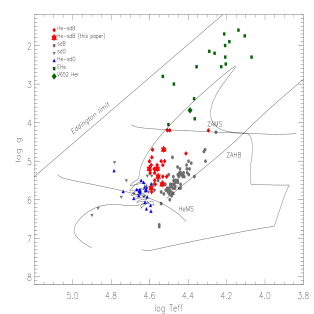
Figure 3: Comparison of hot helium-rich subdwarfs and extreme helium stars with the evolution of a helium white dwarf with $Z=0.001$ following a late helium core flash (Miller Bertolami et al., 2008). The locations of normal sdB’s (Edelmann et al., 2003) He-sdO’s (Ströer et al., 2007), He-sdB’s (Ahmad & Jeffery, 2003), EHe’s (Pandey et al., 2006) and the stars discussed in this paper (N He-sdB) are identified separately (see key). For the latter, we adopt the SFIT results cited in Table 3.

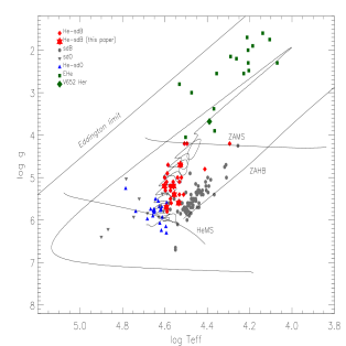
Figure 4: Comparison of hot helium-rich subdwarfs and extreme helium stars with the evolution of a $M_{i}=0.3\,{\rm M_{\odot}}$ helium white dwarf following the accretion of $0.2\,{\rm M_{\odot}}$ helium to represent a double He-WD merger (Saio & Jeffery, 2000). Other symbols as for Fig. 3

4 Evolutionary status of He-sdBs

The evolutionary status of He-sdB and He-sdO stars has been discussed for some three decades. The location of these stars on and above the helium main-sequence points to low-mass helium stars which are either currently in a helium-core burning phase (the helium main sequence), or are approaching or leaving such a phase.

There has been a tendency to analyze and interpret He-sdO (Ströer et al., 2007; Napiwotzki, 2008) and He-sdB stars (Lanz et al., 2004; Ahmad & Jeffery, 2006) separately. This is partly due to the increasing importance of NLTE effects in sdO stars, and hence the adoption of different model atmospheres; a more self-consistent treatment of the two groups would be valuable. The apparent separation of the two groups in $T_{\rm eff}-\log g$ space (Fig. 3) may simply be a consequence of a significant range of $T_{\rm eff}$ within a group of stars having comparable luminosities. Nevertheless, it is clear that extremely helium-rich subdwarfs mark out a clear locus in this diagram, and that they are more luminous than the extended horizontal branch where hydrogen-rich sdB stars are generally found. In addition, there are a small number of cooler helium-rich stars, including V652 Her and BX Cir which may be closely linked to the helium-rich subdwarfs (He-sd’s).

The question of binarity is unresolved. The prototype He-sdB star PG1544+488 is a binary consisting of two He-sdB stars (Ahmad et al., 2004). Only one other binary He-sd, the double He-sdO star HE 0301–3039 (Lisker et al., 2004) has been reported. In such cases the extreme surface composition is a clear consequence of a close binary interaction, probably following a common-envelope phase, in which the entire hydrogen-rich envelope has been ejected. The question is then what differentiates the production of an He-rich subdwarf from a conventional H-rich sdB star in a close binary. Justham et al. (2010) propose a possible evolution following a double-core common-envelope phase involving intermediate mass stars.

In the case of a close binary where envelope ejection exposes CNO-processed helium, the enhancement of nitrogen is easily explained by the conversion, and hence depletion, of carbon and oxygen in the CNO-cycle. A similar abundance pattern is exhibited by the low-luminosity EHe star V652 Her (Jeffery et al., 1999).

N-rich He-sd’s are less easy to explain in the absence of a binary companion. Equally problematic is C-enrichment in either the single- or binary-star cases, since it requires the addition of carbon from $3\alpha$-burning. The low-$L$ EHe star BX Cir (Drilling et al., 1998) provides a C-rich analogy to V652 Her. Neon is normally produced by $\alpha$-captures onto ¹⁴N. Since both are plentiful in CNO-processed helium, a high-temperature episode in the formation of the He-sd might naturally give rise to an overabundance of neon.

Three evolutionary models have been proposed to address these questions for single He-sd’s.

4.1 The late hot flasher

Brown et al. (2001) proposed that single star evolution with enhanced mass loss close to the tip of the RGB will produce a star that suffers its helium-core flash late on the white dwarf cooling track. Since the flash occurs off-center and when the outer layers are compact, flash-driven convection leads to mixing of the remnant H-envelope with the helium core, and possibly also with some carbon from the He-flash itself. The star initially expands to become a yellow giant, and then contracts towards the He main sequence as the helium-burning layers migrates to the center of the star. Subsequent calculations have examined a number of variants of this model (Miller Bertolami et al., 2008) (Fig. 3). The result is either a N-rich or a C-rich He-sdB.

4.2 The double helium white dwarf merger

The merger of two helium white dwarfs has been proposed variously to account for both normal and helium-rich hot subdwarfs (Webbink, 1984; Iben, 1990; Tutukov & Yungel’Son, 1990; Saio & Jeffery, 2000). The progenitors are considered to be short-period systems from which most of the hydrogen and angular momentum has been ejected during a common-envelope phase. The surviving mass of hydrogen is very small relative to the total mixed mass (i.e. that of the disrupted white dwarf) $m_{\rm He}/m_{\rm mixed}\gtrsim 1.4\times 10^{-4}/0.296$ Iben & Tutukov (1986), where the hydrogen mass fraction would probably increase for lower mass white dwarfs.

Saio & Jeffery (2000) investigated the evolution of a helium white dwarf which rapidly accretes helium, i.e. as a result of merger with another helium white dwarf. Following off-center helium ignition, the star expands to become a yellow giant, and then contracts as the helium shell burns inward through a series of mild flashes. The stable end-state of such an evolution would most probably be an He-sdB or He-sdO star. The surface layers of such a star should be dominated by the nitrogen-enriched helium from the disrupted helium white dwarf. Saio & Jeffery (2000) found no evidence for surface carbon enrichment since each shell flash produces very little carbon and the subsequent flash-driven convection reaches the surface only after the first He-shell flash. The evolutionary track from one such model is shown in Fig. 4. Saio & Jeffery (2000) found that one such model would successfully account for the observed properties of the pulsating EHe star V652 Her, which must be in the shell-flashing phase.

4.3 The helium white dwarf plus hot subdwarf merger

Justham et al. (2010) have proposed a model in which a close binary containing a post-sdB star and a helium white dwarf merge. The post-sdB star is essentially a $0.46\,{\rm M_{\odot}}$ hybrid white dwarf containing a small ($\approx 0.3\,{\rm M_{\odot}}$) carbon-oxygen core and a helium envelope. The addition of fresh helium reignites the helium shell, and returns the star close to the helium main-sequence with a helium-rich surface. Population synthesis calculations yield a $T_{\rm eff}-\log g$ distribution similar to that of the He-sdO stars of Ströer et al. (2007).

4.4 Evolutionary status of He-sdB stars

Comparison of the locus of He-sdB stars analysed here and by Ahmad & Jeffery (2003) with the evolutionary calculations discussed above (Figs. 3 and 4) suggests that only the double helium white dwarf merger model successfully accounts for the distribution and surface composition of the N-rich He-sdBs. However, the evolution of both late hot flashers and white dwarf mergers is affected strongly by the metallicity, mass and envelope hydrogen content. Further exploration of the parameter space and of population statistics will be necessary to explain the origins of these evolved stars.

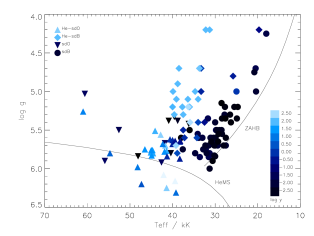
Figure 5: Distribution of helium abundance versus $T_{\rm eff}$ and $\log g$. The helium abundance $\log y=\log(n_{\rm He}/n_{\rm H})$ is indicated by colour (or grey-scale) as shown in the key. The data shown include the He-sdB, He-sdO, sdB and sdO atars from Figs. 3 and 4.

4.5 Surface-chemistry evolution in He-sdB stars

In all of the above evolutionary models, the initial surface composition might be assumed to be determined by the mean mass fractions obtained by combining several layers of stellar material.

For example, the surface of the double helium white-dwarf merger would comprise any surviving hydrogen on the progenitor white dwarfs mixed with the helium core of the less massive component. The surface hydrogen to helium ratio (by mass) would then correspond roughly to the mass ratio of the hydrogen and helium layers in the latter, i.e. $\approx 5\times 10^{-4}$ (see above, $\equiv 2\times 10^{-3}$ by number). Meanwhile the CNO abundances would lie somewhere between a fully CNO-cycled mixture (i.e. carbon and oxygen converted to nitrogen) and a primordial mixture (i.e. carbon, nitrogen and oxygen scaled to the iron abundance), depending on the helium to hydrogen fraction. Additional carbon might be present if 3$\alpha$ burning occurs during the merger.

The surface of a late-flasher will also be represented by CNO-processed helium, doped by whatever envelope hydrogen remained on the surface of the giant before hydrogen-burning was extinguished. This may be anywhere in the ranges $n_{\rm H}/n_{\rm He}\approx 0.001-0.01$ (shallow mixing) or $10^{-5}-10^{-6}$ (deep mixing) (Miller Bertolami et al., 2008). Carbon-enrichment may occur if flash-driven convection can drive material to the surfce after $3\alpha$ ignition, and if the helium-envelope mass is small compared with the amount of carbon available for mixing (Cassisi & Vink, 2003; Lanz et al., 2004).

The question is then what happens to this mixture as the star contracts towards the helium main sequence. It is well known that in a radiative stellar atmosphere having a sufficiently high surface gravity, an imbalance between the relative radiative and gravitational forces on individual ions leads to chemical separation of atomic species by the process of diffusion. Diffusion in subdwarf B stars, with $\log g>5.5$ and $25\,000\lesssim T_{\rm eff}/{\rm K}\lesssim 40\,000$ (Heber, 1992) causes hydrogen to float and helium to sink so that observed helium abundances are typically in the range $0.001<n_{\rm He}/n_{\rm H}<0.01$.

At least two factors moderate the instantaneous conversion of a contracting He-sd into a normal H-rich sdB star. The first is that the diffusion timescale is relatively long $\approx 10^{5}$y (Unglaub & Bues, 2001, no stellar wind). The evolution timescale essentially the thermal timescale for the envelope and is $\approx 10^{6}$y for a merger involving a $0.2{\rm M_{\odot}}$ white dwarf (Saio & Jeffery, 2000), or $\approx 10^{4}$y for a late flasher with a $0.02{\rm M_{\odot}}$ remnant envelope (Miller Bertolami et al., 2008).

The second factor is that a stellar wind acts to slow the diffusion process to give a timescale $\approx 10^{6}$y (Unglaub, 2005, 2008). Since winds in hot subdwarfs are radiatively driven, they are luminosity sensitive. Hence diffusion becomes more effective at low luminosity (high gravity). Helium depletion in the photosphere will accelerate as a star contracts towards the zero-age horizontal branch.

In the absence of winds, and if all He-sd’s were formed in the same way with identical envelope masses, one might expect to see a helium abundance gradient along the observed sequence, or at least to see the helium abundance drop as a helium-rich subdwarf contracts across the “wind-line” – some critical luminosity below which diffusion becomes effective at reducing photospheric helium. The fact that the most hydrogen-rich “He-sds” (i.e. BPS CS 22956-0094, JL 87, LS IV$-14^{\circ}116$) are also those closest to the sdB domain might be important in this regard.

To explore such an hypothesis, Fig. 5 shows the distribution of hot subdwarfs as a function of helium abundance $\log y=\log(n_{\rm He}/n_{\rm H})$; the sample is exclusively that given in Figs. 3 and 4. These observations indicate a substantial majority of normal sdB stars with negligible helium, a significant number of extremely He-rich stars on the pre-subdwarf cooling track and a continuum of hot subdwarfs with relatively high gravities and intermediate helium abundances ($-1<\log y<+1$). In numerical terms, there are roughly 100 normal sdBs for every ten helium-rich plus intermediate-helium subdwarfs (Green et al., 1986), and eighteen helium-rich He-sdBs for nine intermediate He-sdBs (Fig. 5); better statistics would be valuable.

Hot subdwarfs with intermediate helium abundances might then represent stars in which diffusion has started to operate, but in which some helium remains visible. The ratio of intermediate helium subdwarfs to normal subdwarfs should then be given approximately by the ratio of the diffusion timescale ($\approx 10^{6}$ y) to the sdB nuclear timescale ($\approx 10^{8}$ y) times the fraction of sdB stars formed through channels which involve a helium-rich progenitor ($\lesssim 0.5$), leading to a total of roughly one intermediate helium subdwarf in one hundred, slightly fewer than observed.

One problem with this argument, and there are many, is that helium-rich sdB stars may simply become helium-rich sdO stars on the helium main sequence and may not evolve into helium-poor sdB stars. A more detailed examination of surface abundances of other species, including iron, in several helium-rich hot subdwarfs will be necessary.

One observation, however, is instructive. Amongst the helium-rich subdwarfs studied by Ahmad & Jeffery (2006), Ströer et al. (2007) and ourselves, stars with intermediate helium abundances lie predominantly at the boundary between the He-poor and He-rich subdwarfs in the $\log g-T_{\rm eff}$ diagram. There are virtually no He-poor subdwarfs significantly above the horizontal branch (Fig. 5), i.e. with $T_{\rm eff}>30\,000{\rm K}$ and $\log g<5.3$. This observation is supported by low-resolution classification surveys (Winter et al., 2006; Drilling et al., 2003). Thus, if subdwarfs evolve onto either the helium main sequence or the extended horizontal branch by contracting from a more expanded configuration, then the only ones which are currently observed to be doing so are helium rich.

5 Conclusion

As part of an extended study of the surface abundances of extremely helium-rich hot subdwarfs, high-resolution optical échelle spectra of the He-sdB stars LB 1766, SB 21, BPS CS 22940–0009, BPS CS 29496–001, BPS CS 22956–0094 and LB 3229 have been presented. Opacity-sampled line-blanketed model atmospheres have been used to derive atmospheric properties and surface abundances.

All the stars analysed are moderately metal poor compared with the Sun ([Fe/H]$\approx$–0.5). LB 1766 and SB 21, BPS CS 29496–001 and LB 3229 are nitrogen-rich He-sdBs, while BPS CS 22940–0009 and BPS CS 22956–0094 are carbon-rich He-sdBs. The former have a surface composition and $L/M$ ratio comparable with the extreme helium star V652 Her, while the latter might be more directly compared with the extreme helium star BX Cir.

The evolutionary status of He-sdB’s has been discussed in the context of i) close-binary star evolution, ii) a late helium flash in a post-RGB star, iii) the merger of two helium white dwarfs, and iv) the merger of a helium white dwarf with a post-sdB star. The surface composition and locus of single N-rich He-sdBs are currently best explained by the merger of two helium white dwarfs, although this may not necessarily be an unique solution. The merger of a helium white dwarf with a post-sdB white dwarf offers an interesting alternative. C-rich He-sdBs require further investigation; the origin of surface carbon is difficult to explain without mixing $3\alpha$ products to the surface and so far, only the late flasher model seems capable of this. An over-abundance of neon requires further explanation.

On the basis of any of these evolution tracks, the EHe stars V652 Her and BX Cir are likely to evolve to become He-sdB stars. He-sdB stars are likely to evolve to become He-sdO stars.

Appendix A Online Material

Table 4: Oscillator strength ($\log gf$), measured equivalent width ($w_{\lambda}$) and derived elemental abundance $\epsilon_{i}$ for each line measured in the six programme stars.

Ion		LB 1766		SB 21		BPS 22940–0009		BPS 29496–0010		BPS 22956–0094		LB 3229
$\lambda({\rm\AA})$	$\log gf$	$w_{\lambda}({\rm m\AA})$	$\epsilon_{i}$	$w_{\lambda}({\rm m\AA})$	$\epsilon_{i}$	$w_{\lambda}({\rm m\AA})$	$\epsilon_{i}$	$w_{\lambda}({\rm m\AA})$	$\epsilon_{i}$	$w_{\lambda}({\rm m\AA})$	$\epsilon_{i}$	$w_{\lambda}({\rm m\AA})$	$\epsilon_{i}$
C ii
4267.02	0.559$\rceil$					490	9.21			398	8.74
4267.27	0.734$\rfloor$
4074.52	0.408$\rceil$					276	9.13			123	8.49
4074.85	0.593$\rfloor$
4075.94	-0.076$\rceil$					350	8.90			200	8.47
4075.85	0.756$\rfloor$
4074.48	0.204					291	9.19			123	8.49
4374.27	0.634					169	9.05			75	8.52
C iii
4647.42	0.072	100	7.27	31	6.61	380	9.04	65	6.97	189	8.35	90	7.22
4650.25	-0.149	52	6.94	33	6.86	262	8.71	35	6.80	136	8.16	83	7.37
4651.47	-0.625					256	9.15			121	8.51	80	7.82
4067.94	0.827					231	8.30			73	7.64
4068.91	0.945					171	7.94
4070.26	1.037					194	8.97			153	8.99
4186.90	0.924					252	9.16			222	9.15	64	7.64
4156.74	0.8421					170	8.65			140	8.96
4162.87	0.218					140	8.99			170	9.60
N ii
3995.00	0.225	125	8.14	110	7.94	146	8.25	189	8.91	124	8.18	84	8.67
4041.31	0.830	103	8.07	134	8.19	109	8.10	150	8.48	136	8.35	80	8.71
4043.53	0.714	76	7.94	107	8.11	108	8.21	81	8.13	85	8.07	46	8.46
4056.90	-0.461	28	8.51	31	8.50
4073.05	-0.160	53	8.56	77	8.72
4171.59	0.281	48	8.09	70	8.24	70	8.30	49	8.28	41	8.06
4176.16	0.600	79	8.09	85	8.05	119	8.43	65	8.12	80	8.15	70	8.86
4236.98	0.567	139	8.66	135	8.51	126	8.55	143	8.74	161	8.82	63	8.83
4241.78	0.728	179	8.78	83	7.95	101	8.17	128	8.49	98	8.21	105	9.06
4447.03	0.238	59	7.85	65	7.88	100	8.21	94	8.47	118	8.53	85	8.98
4530.40	0.671	84	8.17	83	8.08	122	8.49	128	8.60	100	8.36
4643.09	-0.385	78	8.37	80	8.35	117	8.66			74	8.39
4630.54	0.093	96	8.07	103	8.11	139	8.37	63	8.02	97	8.15
4621.29	-0.483	74	8.42	64	8.27					73	8.48
4613.87	-0.607	71	8.51	74	8.50	91	8.63	57	8.64	82	8.69
4601.48	-0.385	83	8.41	70	8.24	126	8.74	66	8.52	98	8.63
4607.16	-0.483	83	8.41	85	8.50	122	8.80	62	8.57	64	8.38
N iii
4097.33	-0.066	169	8.15	144	8.14	211	8.42	229	8.51	110	7.97	187	8.09
4103.43	-0.377	133	8.14	112	8.16	216	8.77	225	8.80			243	8.86
4640.64	0.140	162	8.40	104	8.15	200	8.58	155	8.30	113	8.38	227	8.51
4634.14	-0.108	135	8.45	110	8.47	170	8.64	174	8.70	63	8.11	186	8.50
4195.762	-0.018	83	8.82	72	8.88							109	8.74
4200.102	0.241	92	8.67	89	8.84					65	8.73	85	8.24
4641.85	-0.815											95	8.44
O  ii
4649.14	0.342	31	7.08	44	7.26	24	6.87
4414.90	0.210	30	7.25	38	7.34
4072.15	0.552	21	7.06	24	7.09	40	7.35
4416.973		61	7.92	55	7.82
4075.86				49	7.33
Ne ii
4219.76	-0.150	40	8.65	75	9.03	55	8.82					40	9.16
4231.60	-0.450	39	8.94	39	8.95
4430.90	-0.609	43	9.22	28	9.00	24	8.87
4397.94	-0.160	35	8.63	36	8.66
4409.29	0.680	55	8.08	55	8.08	53	8.03					35	8.30
4413.20	0.550	35	7.94	34	7.94	48	8.10
4290.37	0.920$\rceil$	100	8.77	63	8.13	45	7.91					58	8.50
4290.60	0.830$\rfloor$

$gf$ values: Cii Yan et al. (1987), Ciii Hibbert (1976); Hardorp. & Scholz (1970); Bockasten (1955), Nii Becker & Butler (1990), Niii Butler (1984), Oii Becker & Butler (1988), Neii Wiese et al. (1966)

Notes: 1: empirical oscillator strength to match observed line; not used in mean. 2: blended with Nii; not used in mean, except for LB 3229 where Nii is weak. 3: possibly blended; not used in mean.

Table 4: contd.

Ion		LB 1766		SB 21		BPS 22940–0009		BPS 29496–0010		BPS 22956–0094		LB 3229
$\lambda({\rm\AA})$	$\log gf$	$w_{\lambda}({\rm m\AA})$	$\epsilon_{i}$	$w_{\lambda}({\rm m\AA})$	$\epsilon_{i}$	$w_{\lambda}({\rm m\AA})$	$\epsilon_{i}$	$w_{\lambda}({\rm m\AA})$	$\epsilon_{i}$	$w_{\lambda}({\rm m\AA})$	$\epsilon_{i}$	$w_{\lambda}({\rm m\AA})$	$\epsilon_{i}$
Mg ii
4481.13	0.568	61	7.17	77	7.24	88	7.27	135	7.80	76	7.22	114	8.21
Al iii
4512.54	0.405	40	6.34	34	6.21	29	6.10
4529.20	0.660	38	6.05	54	6.22	49	6.14
Si iii
4552.62	0.283	114	6.96	114	6.88	164	7.25	75	6.99	104	6.90
4567.82	0.061	82	6.91	69	6.71	138	7.28	67	7.14	75	6.87
4574.76	-0.416	59	7.16	60	7.09	98	7.43			39	6.94
4828.96	0.924	64	7.07
4819.72	0.814	68	7.22
4813.30	0.702	53	7.18
Si iv
4088.85	0.199	143	6.70	123	6.72	237	7.35	139	6.77	97	6.58	250	7.71
4116.10	-0.103	147	7.04	129	7.09	136	6.82	167	7.32	89	6.80	157	7.26
4654.14	1.486			159	7.41							155	7.32
4212.41	0.804											71	7.24
S  iii
4253.59	0.233	78	6.78	51	6.46	60	6.47	31	6.55	82	6.91
4284.99	-0.046	33	6.52	32	6.48	31	6.38	25	6.74	60	6.97
4332.71	-0.393	31	6.83	25	6.70	20	6.50			36	7.00

$gf$ values: Siiii Becker & Butler (1989); Hardorp. & Scholz (1970), Siiv Becker & Butler (1989); Kurucz & Petryemann (1975), Mgii Wiese et al. (1966), Oii Becker & Butler (1988), Aliii Canuto, & Mendoza (1969); McEachran & Cohen (1983), Siii Wiese et al. (1969); Hardorp. & Scholz (1970)

Table 5: Abundance errors $\delta\epsilon_{i}$ due to errors in $T_{\rm eff}$ and $\log g$.

Star	$\delta\epsilon_{i}$
	C	N	O	Ne	Mg	Al	Si	S
BPS 22940–0009
$\delta T_{\rm eff}=1000\,\rm K$	+0.03	+0.06	+0.11	+ 0.05	+0.08	+0.10	+0.08	+0.14
$\delta\log g=0.2$	+0.008	+0.004	–0.02	+0.01	–0.03	–0.02	+0.02	–0.02
LB 1766
$\delta T_{\rm eff}=1000\,\rm K$	–0.07	+0.09	+0.11	+0.05	+0.08	+0.09	+0.10	+0.14
$\delta\log g=0.2$	+0.10	+0.004	–0.03	+0.008	–0.04	–0.04	–0.02	–0.03
LB 3229
$\delta T_{\rm eff}=1000\,\rm K$	+0.10	+0.16		+0.17	+0.19		+0.11
$\delta\log g=0.2$	–0.04	–0.09		–0.10	–0.12		–0.04

Figure 6: The AAT spectrum of LB 1766 along with the best-fit model of $T_{\rm eff}=36\,000\,{\rm K}$, $\log g=5.0$, $n_{\rm He}=0.999$, $v\sin i=20\,{\rm km\,s^{-1}}$, and $v_{\rm t}=10\,{\rm km\,s^{-1}}$. Abundances are as in Table 3.

Figure 7: The AAT spectrum of SB 21 along with the best-fit model of $T_{\rm eff}=36\,000\,{\rm K}$, $\log g=5.5$, $n_{\rm He}=0.999$, $v\sin i=12\,{\rm km\,s^{-1}}$, and $v_{\rm t}=10\,{\rm km\,s^{-1}}$. Abundances are as in Table 3.

Figure 8: The AAT spectrum of LB 3229 along with the best-fit model of $T_{\rm eff}=40\,000\,{\rm K}$, $\log g=5.0$, $n_{\rm He}=0.989$, $v\sin i=8.5\,{\rm km\,s^{-1}}$, and $v_{\rm t}=10\,{\rm km\,s^{-1}}$. Abundances are as in Table 3.

Figure 9: The AAT spectrum of BPS 22940–0009 along with the best-fit model of $T_{\rm eff}=34\,000\,{\rm K}$, $\log g=4.5$, $n_{\rm He}=0.989$, $v\sin i=4\,{\rm km\,s^{-1}}$, and $v_{\rm t}=10\,{\rm km\,s^{-1}}$. Abundances are as in Table 3.

Figure 10: The AAT spectrum of BPS 22956–0094 along with the best-fit model of $T_{\rm eff}=34\,000\,{\rm K}$, $\log g=5.5$, $n_{\rm He}=0.699$, $v\sin i=2\,{\rm km\,s^{-1}}$, and $v_{\rm t}=5\,{\rm km\,s^{-1}}$. Abundances are as in Table 3.

Figure 11: The AAT spectrum of BPS 29496–0010 along with the best-fit model of $T_{\rm eff}=40\,000\,{\rm K}$, $\log g=5.5$, $n_{\rm He}=0.999$, $v\sin i=2\,{\rm km\,s^{-1}}$, and $v_{\rm t}=10\,{\rm km\,s^{-1}}$. Abundances are as in Table 3.

References

- Ahmad et al. (2007) Ahmad A., Behara N. T., Jeffery C. S., Sahin T., Woolf V. M., 2007, A&A, 465, 541
- Ahmad & Jeffery (2003) Ahmad A., Jeffery C. S., 2003, A&A, 402, 335
- Ahmad & Jeffery (2004) Ahmad A., Jeffery C. S., 2004, Ap&SS, 291, 253
- Ahmad & Jeffery (2006) Ahmad A., Jeffery C. S., 2006, Baltic Astronomy, 15, 139
- Ahmad et al. (2004) Ahmad A., Jeffery C. S., Fullerton A. W., 2004, A&A, 418, 275
- Beauchamp & Wesemael (1998) Beauchamp A., Wesemael F., 1998, ApJ, 496, 395
- Becker & Butler (1988) Becker S. R., Butler K., 1988, A&A, 209, 244
- Becker & Butler (1989) Becker S. R., Butler K., 1989, A&A, 201, 232
- Becker & Butler (1990) Becker S. R., Butler K., 1990, A&A, 235, 326
- Beers et al. (1992) Beers T. C., Doinidis S. P., Griffin K. E., Preston G. W., Shectman S. A., 1992, AJ, 103, 267
- Behara & Jeffery (2006) Behara N. T., Jeffery C. S., 2006, A&A, 451, 643
- Bockasten (1955) Bockasten K., 1955, Ark. Fys., 9, 457
- Brown et al. (2001) Brown T. M., Sweigart A. V., Lanz T., Landsman W. B., Hubeny I., 2001, ApJ, 562, 368
- Butler (1984) Butler K., 1984, PhD Thesis, University College London
- Canuto, & Mendoza (1969) Canuto, W., Mendoza C., 1969, Mexicana Astron. Astrofis, 23, 107
- Cassisi & Vink (2003) Cassisi S., Vink J. S., 2003, in G. Piotto, G. Meylan, S. G. Djorgovski, & M. Riello ed., New Horizons in Globular Cluster Astronomy Vol. 296 of Astronomical Society of the Pacific Conference Series, Mass Loss Predictions for Hot Horizontal Branch Stars. pp 201–+
- Drilling et al. (1998) Drilling J. S., Jeffery C. S., Heber U., 1998, A&A, 329, 1019
- Drilling et al. (2003) Drilling J. S., Moehler S., Jeffery C. S., Heber U., Napiwotzki R., 2003, in R. O. Gray, C. J. Corbally, & A. G. D. Philip ed., The Garrison Festschrift Spectral Classification of Hot Subdwarfs. pp 27–+
- Dziembowski (1998) Dziembowski W. A., 1998, Space Science Reviews, 85, 37
- Edelmann et al. (2003) Edelmann H., Heber U., Hagen H., Lemke M., Dreizler S., Napiwotzki R., Engels D., 2003, A&A, 400, 939
- Green et al. (1986) Green R. F., Schmidt M., Liebert J., 1986, ApJS, 61, 305
- Grevesse & Sauval (1998) Grevesse N., Sauval A. J., 1998, Space Science Reviews, 85, 161
- Hardorp. & Scholz (1970) Hardorp. Scholz 1970, Astrophys.J.Supp, 19, 193
- Harrison & Jeffery (1997) Harrison P. M., Jeffery C. S., 1997, A&A, 323, 177
- Heber (1986) Heber U., 1986, A&A, 155, 33
- Heber (1992) Heber U., 1992, in U. Heber & C. S. Jeffery ed., The Atmospheres of Early-Type Stars Vol. 401 of Lecture Notes in Physics, Berlin Springer Verlag, Hot subluminous stars (review). pp 233–+
- Heber (2009) Heber U., 2009, ARA&A, 47, 211
- Hibbert (1976) Hibbert A., 1976, J.Phys.B, 9, 2805
- Hunger et al. (1981) Hunger K., Gruschinske J., Kudritzki R. P., Simon K. P., 1981, A&A, 95, 244
- Hunger & Kudritzki (1980) Hunger K., Kudritzki R. P., 1980, A&A, 88, L4
- Iben & Tutukov (1986) Iben Jr. I., Tutukov A. V., 1986, ApJ, 311, 742
- Iben (1990) Iben I. J., 1990, ApJ, 353, 215
- Jeffery (1996) Jeffery C. S., 1996, in Jeffery C. S., Heber U., eds, Hydrogen Deficient Stars Vol. 96 of Astronomical Society of the Pacific Conference Series, Surface properties of extreme helium stars. p. 152
- Jeffery (2008a) Jeffery C. S., 2008a, in Werner A., Rauch T., eds, Hydrogen-Deficient Stars Vol. 391 of Astronomical Society of the Pacific Conference Series, Hydrogen-Deficient Stars: An Introduction. p. 3
- Jeffery (2008b) Jeffery C. S., 2008b, Information Bulletin on Variable Stars, 5817, 1
- Jeffery et al. (1999) Jeffery C. S., Hill P. W., Heber U., 1999, A&A, 346, 491
- Jeffery et al. (2001) Jeffery C. S., Woolf V. M., Pollacco D. L., 2001, A&A, 376, 497
- Justham et al. (2010) Justham S., Podsiadlowski P., Han Z., Wolf C., 2010, Ap&SS, p. 116
- Klemola (1961) Klemola A. R., 1961, ApJ, 134, 130
- Kurucz & Petryemann (1975) Kurucz R., Petryemann E., 1975, SAO Spec.Rep, 362
- Lanz et al. (2004) Lanz T., Brown T. M., Sweigart A. V., Hubeny I., Landsman W. B., 2004, ApJ, 602, 342
- Leuenhagen et al. (1996) Leuenhagen U., Hamann W.-R., Jeffery C. S., 1996, A&A, 312, 167
- Lisker et al. (2004) Lisker T., Heber U., Napiwotzki R., Christlieb N., Reimers D., Homeier D., 2004, Ap&SS, 291, 351
- McEachran & Cohen (1983) McEachran R., Cohen M., 1983, J.Phys.B, 16, 3125
- Miller Bertolami et al. (2008) Miller Bertolami M. M., Althaus L. G., Unglaub K., Weiss A., 2008, A&A, 491, 253
- Mills et al. (2006) Mills D., Webb J., Clayton W., 2006, Starlink User Note, 152
- Moehler et al. (1990) Moehler S., Richtler T., de Boer K. S., Dettmar R. J., Heber U., 1990, A&AS, 86, 53
- Napiwotzki (2008) Napiwotzki R., 2008, in Werner A., Rauch T., eds, Hydrogen-deficient stars Vol. 391 of Astron. Soc. Pac. Conf. Ser., The Origin of Helium-Rich Subdwarf O Stars. p. 257
- Naslim et al. (2010) Naslim N., Jeffery C., Hibbert A., Behara N., 2010, MNRAS, In preparation
- Naslim et al. (2010) Naslim N., Jeffery C. S., Ahmad A., Behara N., Şahın T., 2010, Ap&SS, p. 89
- Pandey et al. (2006) Pandey G., Lambert D. L., Jeffery C. S., Rao N. K., 2006, ApJ, 638, 454
- Saio & Jeffery (2000) Saio H., Jeffery C. S., 2000, MNRAS, 313, 671
- SŞahìn (2008) SŞahìn T., 2008, PhD thesis, Queens University Belfast
- Ströer et al. (2007) Ströer A., Heber U., Lisker T., Napiwotzki R., Dreizler S., Christlieb N., Reimers D., 2007, A&A, 462, 269
- Tutukov & Yungel’Son (1990) Tutukov A. V., Yungel’Son L. R., 1990, Astron.Zh., 67, 109
- Underhill (1966) Underhill A., 1966, The Early Type Stars. D. Reidel, Dordrecht, Holland
- Unglaub (2005) Unglaub K., 2005, in D. Koester & S. Moehler ed., 14th European Workshop on White Dwarfs Vol. 334 of Astronomical Society of the Pacific Conference Series, The Upward Diffusion of Hydrogen in Helium-Rich Subdwarf B Stars. pp 297–+
- Unglaub (2008) Unglaub K., 2008, A&A, 486, 923
- Unglaub & Bues (2001) Unglaub K., Bues I., 2001, A&A, 374, 570
- Webbink (1984) Webbink R. F., 1984, ApJ, 277, 355
- Wiese et al. (1966) Wiese W., Smith M., Glennon 1966, National Bureau of Standards (USA) Publs, I-II
- Wiese et al. (1969) Wiese W., Smith M., Miles B., 1969, National Bureau of Standards (USA) Publs
- Winter et al. (2006) Winter C., Jeffery C. S., Ahmad A., Morgan D. R., 2006, Baltic Astronomy, 15, 69
- Yan et al. (1987) Yan C., Taylor K., Seaton M., 1987, J.Phys.B, 20, 6399