Waves in pulsar winds

Abstract

The radio, optical, X-ray and gamma-ray nebulæ that surround many pulsars are thought to arise from synchrotron and inverse Compton emission. The energy powering this emission, as well as the magnetic fields and relativistic particles, are supplied by a “wind” driven by the central object. The inner parts of the wind can be described using the equations of MHD, but these break down in the outer parts, when the density of charge carriers drops below a critical value. This paper reviews the wave properties of the inner part (striped wind), and uses a relativistic two-fluid model (cold electrons and positrons) to re-examine the nonlinear electromagnetic modes that propagate in the outer parts. It is shown that in a radial wind, two solutions exist for circularly polarised electromagnetic modes. At large distances one of them turns into a freely expanding flow containing a vacuum wave, whereas the other decelerates, corresponding to a confined flow.

1 Introduction

The size and quality of the observational database relating to pulsar wind nebulæ has increased dramatically in the past five years, stimulating research into both the modelling of their spectra and the theory of the winds themselves (for recent reviews see [1, 2]). The basic idea of the pulsar wind as a mix of particles, fields and waves, was outlined over thirty years ago [3]. Close to the pulsar, the wind moves outwards at relativistic speed. When the the ram-pressure drops to approximately that of the surroundings, a “termination shock” occurs, and strong synchrotron and inverse Compton radiation is emitted in the relatively slowly moving plasma in the surrounding “nebula”. However, although progress has been made on understanding the structure of the nebula, [4, 5, 6] there are still difficulties associated with the propagation of the wind. For example, the questions of where and how the Poynting flux that it carries is dissipated into particles remains open [7, 8, 9, 10, 11]. This paper, does not present a solution to these problems, but concerns itself with an analysis of two simple, nonlinear waves that propagate in the wind, and are likely to play a crucial role in shaping the global solution.

A rotating magnetised neutron star can be expected to emit predominantly linearly polarised waves in the equatorial plane, and circularly polarised waves along the rotation axis. In addition, the waves in the equatorial region may carry a non-vanishing phase-averaged component of the magnetic field component. At intermediate latitudes, the waves will, in general, be elliptically polarised and may also carry a non-oscillatory component. A linear analysis of these waves is clearly inadequate, since the characteristic quiver frequency of an electron at points interior to the termination shock front is many orders of magnitude larger than the rotation frequency of the star. A nonlinear analysis, however, is feasible only for a few simple modes.

The first mode we select for analysis is a linearly polarised wave — the striped wind — which has vanishing phase-averaged magnetic field. This wave can be thought of as an entropy wave or, alternatively, a rotational discontinuity. It requires a minimum plasma density in order to propagate, and so can exist only up to some maximum distance from the pulsar. Its subluminal phase velocity equals its group velocity, and the field is essentially magnetostatic in the wave frame. Since it propagates at highly super-magnetosonic velocity, its evolution is fixed by boundary conditions close to the star. This wave is likely to provide a good description of the interior zone of a pulsar wind in the equatorial regions.

Following this, the propagation of nonlinear electromagnetic waves of superluminal phase velocity is addressed. These waves cut off if the plasma density exceeds a certain limit, and so propagate only beyond some minimum distance from the star. Both linearly and circularly polarised nonlinear plane waves can be constructed analytically, but the formalism is much simpler for the case of circular polarisation. In this paper, a new analysis is presented of circularly polarised waves in spherical geometry, using the short wavelength approximation. This is appropriate in the polar regions of a pulsar wind. However, one can expect that the linearly polarised electromagnetic modes in the equatorial region exhibit qualitatively similar behaviour. Because the phase speeds are superluminal, both inner and outer boundary conditions are required to specify the wave structure. At large radius, two types of solution are found: in one of them the flow velocity stagnates in a region of constant density, whereas, in the other, it asymptotes to constant radial velocity. The former applies to pulsar wind nebulae, which are confined by an external medium. The latter applies to unconfined winds.

2 Parameters of the wave

Consider radially propagating waves in a region far outside the light-cylinder of the pulsar, i.e., $\hat{r}=r/r_{\rm L}\gg 1$, where $r_{\rm L}=cP/2\pi$ is the radius of the light cylinder and $P$ is the pulsar period. In this region, the magnetic field is approximately transverse, because the longitudinal (radial) component decays as $\hat{r}^{-2}$, whereas transverse component decays as $\hat{r}^{-1}$. Furthermore, a plane wave approximation is appropriate, since the wavelength is small compared to the curvature of the wavefront. Though approximately radial, pulsar winds are definitely not spherically symmetric, which is accounted for by specifying a finite solid angle $\Omega_{\rm s}<4\pi$ in which the wind propagates.

The wave properties depend on the phase-averaged radial particle flux density $\left<J\right>$, the phase-averaged total radial energy flux density $\left<F\right>$, (which is the component $T^{0,1}$ of the sum of the stress-energy tensors of the fields and particles), and the phase-averaged flux density of radial momentum, $\left<Q\right>$, (which is the component $T^{1,1}$). This latter quantity depends on both $\left<F\right>$ and on the way in which the energy flux is shared between the particles and fields. For example, for a vacuum wave, the momentum flux density equals the energy flux density/c, whereas for cold particles of speed $v$ in the absence of fields the momentum density equals $v/c^{2}$ times the energy flux density.

Instead of the fluxes, however, it is more convenient to use dimensionless parameters. Conventionally, a steady, relativistic MHD wind is characterised by the parameter $\mu$ introduced by Michel [12], which is the luminosity carried by the wind per unit rest mass. It gives the Lorentz factor each particle would have if all the energy flux were carried by the particles:

$$\mu = \frac{\left<F\right>}{mc^{2}\left<J\right>}$$ (1)

In a pulsar wind, $\mu$ is constant, (provided pairs are not created or annihilated and no energy is dissipated into radiation in the region under consideration), but its value is uncertain. For the Crab Nebula the average of $\mu$ over the pulsar lifetime can be found by combining an estimate of the number of radiating electrons/positrons, obtained from the synchrotron luminosity, with an estimate of the average magnetic field, obtained from the gamma-ray luminosity. But the current value is thought by many to be rather higher than in the past. One estimate is $\mu\sim 10^{4}$ [2] but the real value might be larger.

The distribution of energy flux between particles and fields can be described by the magnetisation parameter $\sigma$, defined, in an MHD flow, as the ratio of the enthalpy density of the magnetic field to that of the plasma, measured in the plasma rest frame. This quantity depends on the fraction of the pulsar luminosity that goes into creating pairs, i.e., not only on their number, but also on the Lorentz factor with which they are injected into the wind. $\sigma$ is the ratio of the maximum possible Lorentz factor (the parameter $\mu$) to this injection Lorentz factor. This is generally thought to be high $\sim 10^{2}$–$10^{3}$, so that $\sigma\approx 10^{-2}\mu$–$10^{-3}\mu$.

Finally, as a dimensionless expression of the total energy flux it is convenient to choose the strength parameter of a circularly polarised vacuum wave that carries the same energy flux as the nonlinear wave. Writing $E_{\rm eff}$ for the magnitude of the electric field in this wave, the strength parameter is defined as $a={eE_{\rm eff}}/{(mc\omega)}$, and the required value of $E_{\rm eff}$ is determined from $c{E_{\rm eff}^{2}}/{(4\pi)}=\left<F\right>$:

$$a = \left[\frac{4\pi e^{2}\left<F\right>}{m^{2}c^{3}\omega^{2}}\right]^{1/2}$$ (2)

In a pulsar, this quantity varies with position in the wind: $a=a_{\rm L}/\hat{r}$ where $a_{\rm L}$ is the strength parameter evaluated at $r=r_{\rm L}$:

$$a_{\rm L} = \left[\frac{4\pi e^{2}L}{m^{2}c^{5}\Omega_{\rm s}}\right]^{1/2}$$ (3)

$$= 4.3\times 10^{10}L_{38}^{1/2}\left(4\pi/\Omega_{\rm s}\right)^{1/2}$$

where $L$ is the luminosity carried by the (radial) wind, and $L_{38}=L/(10^{38}\,\textrm{erg\,s}^{-1})$. For the Crab, $L=4.6\times 10^{38}\,\textrm{erg\,s}^{-1}$; many pulsars have $L=10^{31}$ — $10^{33}\,\textrm{erg\,s}^{-1}$, and some go down to $10^{28}\,\textrm{erg\,s}^{-1}$. The value of $\Omega_{\rm s}$ is not known, but is often assumed to be $\sim 1$. In a steady, radial wind,

$$\hat{r}^{2}\left<J\right> = C_{J}$$ (4)

$$\hat{r}^{2}\left<F\right> = mc^{2}C_{F}$$ (5)

$$\hat{r}^{2}\left<Q\right> = mcC_{Q}$$ (6)

where $C_{J,F,Q}$ are constants and $\mu=C_{F}/C_{J}$. The particle density is frequently expressed in units of the “Goldreich-Julian” density at the light cylinder [13]. For a magnetically dominated, relativistic flow, the corresponding “multiplicity” parameter is $\kappa=a_{\rm L}/(4\mu)$.

3 The striped wind — an MHD wave

Coroniti [14] and Michel [15] suggested idealised solutions in which the wind settles down into stripes of magnetic flux of alternating polarity containing cold plasma, separated by current sheets containing hot plasma. In this solution, the plasma is at rest in a reference frame that, with respect to the star, moves radially outwards with Lorentz factor $\gamma_{\rm MHD}=\left(1-\beta_{\rm MHD}^{2}\right)^{-1/2}$. In the comoving frame, the electric field vanishes, and the magnetic field is toroidal. There are two current sheets per wavelength.

Such solutions can exist only if the wind carries a sufficient number of particles to carry the current that Ampere’s law requires must flow in the sheets. To within a factor of the order of unity, this condition is equivalent to the requirement that particles can be confined in the sheet, i.e., that the gyro-radius of a hot particle moving in the magnetic field present in the cold part of the flow is smaller than the sheet thickness. It was noticed in [14] that this condition implies a minimum dissipation rate: as the density decreases radially, the minimum sheet thickness increases. According to [13], dissipation forces the wind to accelerate, which, because of time-dilation, reduces the apparent dissipation rate observed in the lab. frame. Of course, the actual dissipation rate is unknown. If it lies below the minimum, then the solution moves out of the range of validity of the MHD equations. If it lies above the minimum, the sheet expands, consuming the surrounding cold plasma and annihilating the field embedded in it. In the equatorial plane, adjacent sheets carry equal and opposite magnetic fluxes, and it is conceivable that the wave eventually annihilates the entire magnetic field. However, at higher latitudes, a residual flux remains after removal of the alternating component.

Several possible dissipation or “reconnection” scenarios were investigated in [9]. The conclusion, in the case of the Crab, is that the maximum possible dissipation rate, combined with a very high particle content (small $\mu$), could marginally enable the conversion of all the wind energy flux into particle kinetic energy before the termination shock is encountered. Given a reconnection prescription, self-similar solutions can be found that describe how the flow accelerates. For example, for dissipation at the minimum rate, the radial dependence can be approximated by [9]

$$\gamma_{\rm MHD} = \mu\sqrt{3\hat{r}/(\pi a_{\rm L})}$$ (7)

This relation holds in the supersonic part of the flow ($\gamma_{\rm MHD}>\mu^{1/3}$), and before the magnetic field is annihilated completely ($\gamma_{\rm MHD}<\mu$). In terms of the radius, these restrictions imply $a_{\rm L}>\hat{r}>a_{\rm L}/\mu^{4/3}$.

However, there exists an additional, independent constraint that is imposed by the use of a short-wavelength approximation in this analysis. This requires that the striped wind pass through a series of quasi-stationary states as it expands in the radial geometry. For this to remain valid, the gyro-period of particles contained in the sheets must be short compared to the expansion timescale. An equivalent formulation of this condition is that the speed at which the sheet expands must remain subsonic. This implies an upper limit on the wind Lorentz factor, and, hence, the radius:

$$\gamma_{\rm MHD} < \gamma_{\rm M}\,\approx\,a_{\rm L}/\mu\qquad\hat{r}\,<\,a_{\rm L}^{3}/\mu^{4}$$ (8)

above which the wave can no longer be described by the MHD equations.

In order to relate the striped wind solutions, which apply in the inner part of the wind, to the electromagnetic waves to be described in the following section, which apply in the outer part of the wind, it is useful to write down the phase-averaged fluxes carried by the wind, assuming the contribution of the current sheets to be negligible. Noting that the electric and magnetic fields are related by $E=\beta_{\rm MHD}B$, are orthogonal, and are constant in between the current sheets, (although they change sign across each sheet), and that the wave speed equals the fluid speed, i.e., $\gamma_{\rm MHD}=\gamma=\sqrt{1+{p_{\|}}^{2}}$, where $\gamma$ is the particle Lorentz factor and ${p_{\|}}$ the radial momentum in units of $mc$, one finds:

$$\left<J\right> = 2n{p_{\|}}c$$ (9)

$$\left<F\right> = 2nmc^{3}{p_{\|}}\gamma+c\beta_{\rm MHD}\frac{B^{2}}{4\pi}$$ (10)

$$\left<Q\right> = 2nmc^{2}{p_{\|}}^{2}+\left(1+\beta_{\rm MHD}^{2}\right)\frac{B^{2}}{8\pi}$$ (11)

where $n$ is the proper number density of electrons, which equals that of positrons. In terms of the magnetisation parameter, $\sigma=B^{2}/\left(8\pi\gamma_{\rm MHD}^{2}nmc^{2}\right)$:

$$\frac{\left<F\right>}{mc^{2}\left<J\right>} = \frac{C_{F}}{C_{J}}\,\equiv\,\mu\,=\,\gamma_{\rm MHD}\left(1+\sigma\right)$$ (12)

$$\frac{\left<Q\right>}{mc\left<J\right>} = \frac{C_{Q}}{C_{J}}\,=\,\left(\gamma_{\rm MHD}^{2}-1\right)^{-1/2}\left[\gamma_{\rm MHD}^{2}\left(1+\sigma\right)-\left(1+\frac{\sigma}{2}\right)\right]$$ (13)

and so in this case, in which the effect of the current sheets is neglected, both $\gamma_{\rm MHD}$ and $\sigma$ remain constant in the flow. For $\mu\gg 1$ and $\sigma\ll\mu^{2}$, the energy and momentum flux densities are almost equal:

$$\frac{C_{F}}{C_{J}} = \mu;\qquad\frac{C_{Q}}{C_{J}}\,\approx\,\mu-\frac{1+\sigma}{2\mu}$$ (14)

4 Electromagnetic waves

A relatively simple description of the outer parts of a pulsar wind can be based on a model in which two cold, relativistic, fluids (electrons and positrons) propagate radially outwards in transverse electromagnetic fields. Strong waves in systems similar to this were analysed by [16, 17, 18, 19], using the method of [20]. In connection with pulsars [21] and [22] investigated strong, linearly polarised waves in spherical geometry. Here the effect of spherical geometry on circularly polarised electromagnetic waves is analysed.

Under the above assumptions, the proper number density is the same for each fluid: $n_{+}=n_{-}=n$. In spherical polar coordinates $(r,\theta,\phi)$ their radial velocity is also the same: $v_{r+}=v_{r-}=v_{r}$ and the toroidal and azimuthal velocities are equal in magnitude but of opposite sign: $v_{\theta+}=-v_{\theta-}$, $v_{\phi+}=-v_{\phi-}$. It proves convenient to use the Lorentz factor of the fluids $\gamma_{+}=\gamma_{-}=\gamma=c/\sqrt{c^{2}-v_{r}^{2}-v_{\theta+}^{2}-v_{\phi+}^{2}}$, to define the dimensionless radial momentum: ${p_{\|}}=v_{r}\gamma/c$, and to introduce complex quantities representing the dimensionless transverse momentum: ${p_{\bot}}=\left(v_{\theta+}+iv_{\phi+}\right)\gamma/c$ ($=-\left(v_{\theta-}+iv_{\phi-}\right)\gamma/c$) and the electric and magnetic fields: $E=E_{\theta}+iE_{\phi}$, $B=B_{\theta}+iB_{\phi}$. Then the equations to be solved are the continuity equation

$$\frac{\partial}{\partial t}\left(n\gamma\right)+\frac{c}{r^{2}}\frac{\partial}{\partial r}\left(r^{2}n{p_{\|}}\right) = 0$$ (15)

the fluid equations of motion

$$\frac{{\rm d}{p_{\|}}}{{\rm d}\tau} = -\frac{e}{mc}\textrm{Im}\left({p_{\bot}}B^{*}\right)$$ (16)

$$\frac{{\rm d}{p_{\bot}}}{{\rm d}\tau} = \frac{e}{mc}\left(\gamma E+i{p_{\|}}B\right)$$ (17)

$$\frac{{\rm d}\gamma}{{\rm d}\tau} = \frac{e}{mc}\textrm{Re}\left({p_{\bot}}E^{*}\right)$$ (18)

(where $\tau$ is the proper time (${\rm d}t=\gamma{\rm d}\tau$) and ${{\rm d}}/{{\rm d}\tau}={\partial}/{\partial\tau}+c{p_{\|}}{\partial}/{\partial r}$ is the convective derivative), together with Faraday’s law and Ampère’s law:

$$\frac{1}{r}\frac{\partial}{\partial r}\left(rE\right)-\frac{i}{c}\frac{\partial B}{\partial t} = 0$$ (19)

$$\frac{1}{r}\frac{\partial}{\partial r}\left(rB\right)+\frac{i}{c}\frac{\partial E}{\partial t} = -i8\pi ne{p_{\bot}}$$ (20)

In the limit of large $r$, approximate solutions to these equations can be found that describe nonlinear waves, using the method of [20]. Introducing the phase

$$\phi = \omega\left[t-\frac{1}{c}\int_{0}^{r}\frac{{\rm d}r^{\prime}}{\beta\left(r^{\prime}\right)}\right]$$ (21)

one can identify a circularly polarised solution valid for superluminal phase speeds ($\beta>1$). In it, the fields are

$$B = iE/\beta;\qquad E\,=\,\left|E\right|\textrm{e}^{\pm i\phi}$$ (22)

and the two fluids have oppositely directed, non-zero components of momentum perpendicular to the propagation direction, whose magnitude is related to the electric field strength:

$$\left|{p_{\bot}}\right|^{2} = \frac{e^{2}\left|E\right|^{2}}{m^{2}c^{2}\omega^{2}}$$ (23)

$$= \gamma^{2}-{p_{\|}}^{2}-1$$ (24)

where $\left|{p_{\bot}}\right|$ and $\left|E\right|$ are constants. This extra degree of freedom (compared to the subluminal striped wind) brings with it a restriction on the plasma density in the form of a non-linear dispersion relation:

$$\omega = \gamma_{\rm EM}\omega_{\rm p}$$ (25)

where $\omega_{\rm p}=\left(8\pi ne^{2}/m\right)^{1/2}$, and $\gamma_{\rm EM}=\beta/\sqrt{\beta^{2}-1}$ is the Lorentz factor that corresponds to a velocity of $c/\beta$. Seen from a frame moving radially outwards with this speed, the wave is spatially homogeneous and the magnetic field vanishes.

4.1 Perturbation expansion

Applying a short wavelength approximation to the above equations reveals that the slow radial evolution of the wave amplitude is governed by the conservation of particle number, energy and radial momentum.

$$C_{J} = \hat{r}^{2}\left<J\right>\,=\,\hat{r}^{2}2cn{p_{\|}}$$ (26)

$$C_{F} = \frac{\hat{r}^{2}\left<F\right>}{mc^{2}}\,=\,\hat{r}^{2}\left(2nc\gamma{p_{\|}}+\frac{\left|E\right|^{2}}{4\pi mc\beta}\right)$$ (27)

$$C_{Q} = \frac{\hat{r}^{2}\left<Q\right>}{mc}\,=\,\hat{r}^{2}\left[2nc{p_{\|}}^{2}+\frac{\left|E\right|^{2}}{8\pi mc}\left(1+\frac{1}{\beta^{2}}\right)\right]$$ (28)

The dispersion relation (25) implies that the proper density is proportional to $\gamma_{\rm EM}^{-2}$. Therefore, because of the conservation of particle flux, ${p_{\|}}\propto\gamma_{\rm EM}^{2}/\hat{r}^{2}$. The constant of proportionality is not important for the analysis of the wave properties, but it can be found from the spin-down power:

$${p_{\|}} = \frac{a_{\rm L}^{2}\gamma_{\rm EM}^{2}}{\mu\hat{r}^{2}}$$ (29)

where $a_{\rm L}$ is the strength parameter defined in (3). As a result of (29), this wave propagates only at a sufficiently large distance from the star. Since ${p_{\|}}<\gamma<\mu$, the wave propagates only for

$$\hat{r} > \frac{a_{\rm L}\gamma_{\rm EM}}{\mu}\,>\,\frac{a_{\rm L}}{\mu}$$ (30)

$$= 4.3\times 10^{6}\mu_{4}^{-1}L_{38}^{1/2}\left(4\pi/\Omega_{\rm s}\right)^{1/2}$$

where $\mu_{4}=\mu/10^{4}$. In the following, the dimensionless radius will be expressed in terms of this minimum radius for propagation, using the variable

$$R = \hat{r}\mu/a_{\rm L}$$ (31)

From (26) and (27) the $\mu$ parameter is

$$\mu = \frac{\left<F\right>}{mc^{2}\left<J\right>}$$ (32)

$$= \gamma+\frac{\left|E\right|^{2}}{8\pi\beta nmc^{2}{p_{\|}}}$$

$$= \gamma+\frac{\gamma_{\rm EM}^{2}{p_{\bot}}^{2}}{\beta{p_{\|}}}$$ (33)

where the dispersion relation (25) has been used in the last step. Similarly, from (26) and (28) one finds

$$\frac{C_{Q}}{C_{J}} = {p_{\|}}+\frac{\gamma_{\rm EM}^{2}{p_{\bot}}^{2}}{2{p_{\|}}}\left(1+\frac{1}{\beta^{2}}\right)$$ (34)

The radial dependence of the wave follows from (33) and (34), together with

$${p_{\|}} = \frac{\gamma_{\rm EM}^{2}\mu}{R^{2}}$$ (35)

$$\gamma^{2} = 1+{p_{\|}}^{2}+{p_{\bot}}^{2}$$ (36)

$$\beta = \frac{\gamma_{\rm EM}}{\sqrt{\gamma_{\rm EM}^{2}-1}}$$ (37)

Using (34) to eliminate ${p_{\bot}}$ in (33) enables one to find a quadratic equation for ${p_{\|}}$, so that for a given wave speed $\gamma_{\rm EM}$, there are at most two distinct physical solutions for ${p_{\|}}$ and, hence, for the radius. In order to relate these solutions to the striped wind solutions that carry the same particle, energy and momentum fluxes, it suffices to express $C_{Q}/C_{J}$ in terms of the magnetisation parameter $\sigma$ using (13) The radial dependence of these two modes for $\mu=10^{4}$ and $\sigma=10^{2}$ is shown in Fig. 1.

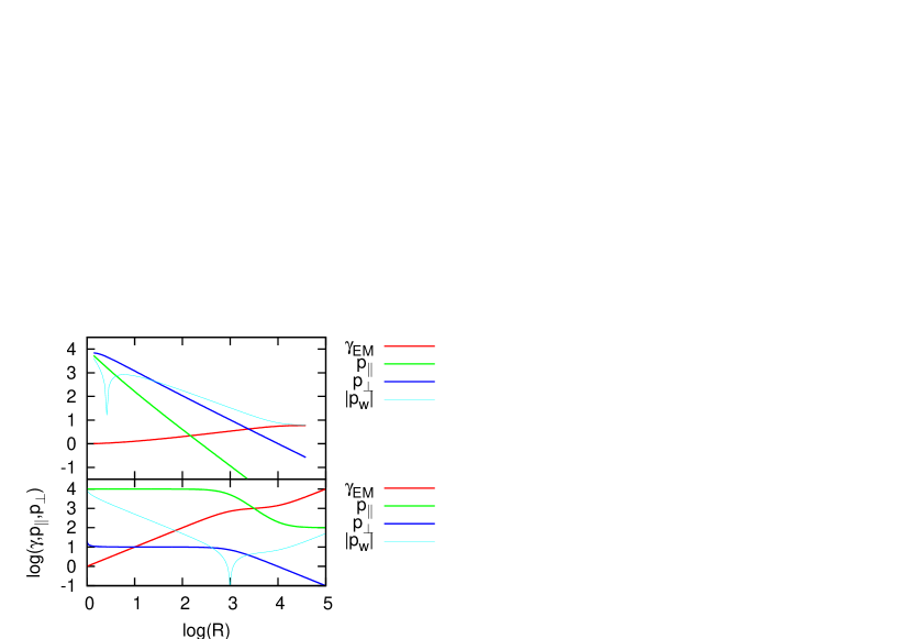
Figure 1: The properties of circularly polarised EM waves for $\mu=10^{4}$, $\sigma=10^{2}$. The quantity $p_{\rm w}$ is the radial momentum of the electron and positron fluids seen from the wave frame. It is positive (wave slower than particles) at $R=1$, but becomes negative at large $R$.

To find the behaviour at large radius, first write an expression for ${p_{\bot}}$, using (34) and (35):

$${p_{\bot}}^{2} = \frac{2\mu\gamma_{\rm EM}^{2}}{R^{2}\left(2\gamma_{\rm EM}^{2}-1\right)}\left[\mu\left(1-\frac{\gamma_{\rm EM}^{2}}{R^{2}}\right)-\frac{1+\sigma}{2\mu}\right]$$ (38)

As $R\rightarrow\infty$, $\gamma_{\rm EM}$ cannot rise faster than $R$, since ${p_{\|}}<\mu$. Therefore, for both modes, ${p_{\bot}}\sim R^{-1}$, i.e., the wave amplitude decreases as $1/R$.

4.2 Free-escape mode

Writing $\gamma_{\rm EM}=yR$ and expanding in powers of $1/R$ gives

$$y = \frac{1}{\sqrt{1+\sigma}}\left[1-\left(\frac{1+\sigma}{2\mu}\right)^{2}\right]^{1/2}\ \textrm{as}\ R\rightarrow\infty$$ (39)

Assuming $\mu/(1+\sigma)\gg 1$, this mode has the properties

$$\gamma_{\rm EM} \rightarrow R/\sqrt{1+\sigma}$$ (40)

$${p_{\bot}} \rightarrow \frac{\mu\sqrt{\sigma}}{R\left(1+\sigma\right)^{1/2}}$$ (41)

$${p_{\|}} \rightarrow \frac{\mu}{1+\sigma}$$ (42)

as $R\rightarrow\infty$. At large distances, its Lorentz factor increases linearly with $R$, but the radial momentum of the particles tends to a constant, so that the density falls of as $R^{-2}$. The wave essentially detaches itself from the particles, and becomes a vacuum wave with a frequency large compared to the local plasma frequency. Most of the energy flux at large radius is carried by the wave, in the sense that the ratio of the two terms on the RHS of (33) is $\left[\gamma_{\rm EM}^{2}{p_{\bot}}^{2}/\left(\beta{p_{\|}}\right)\right]/\gamma=\sigma\gg 1$. Thus, the ratio of electromagnetic to particle energy flux tends to the same value as in the MHD wave that carries the same total particle, energy and momentum fluxes.

At smaller radius, this mode changes character, roughly at the point where the wave Lorentz factor equals that of the particles, i.e., $R\approx\mu/\sqrt{1+\sigma}$. Inside this point, the wave moves outwards more slowly than the particles. Since ${p_{\|}}\approx\gamma\approx\mu$, most of the energy flux in this inner region is carried by the particles. The wave amplitude ${p_{\bot}}$ is nearly constant.

4.3 Confined mode

The second mode is very different. At large radius, $\gamma_{\rm EM}$ tends to a constant, ${p_{\|}}\rightarrow 0$ and $\gamma\rightarrow 1$. In this case, combining (33) and (34) for large $R$ leads to

$$\mu-\frac{1+\sigma}{2\mu} = \beta(\mu-1)\frac{1}{2}\left(1+\frac{1}{\beta^{2}}\right)$$ (43)

This equation has one superluminal ($\beta>1$) root provided $\mu>(1+\sigma)/2$, as is expected under pulsar conditions. For large $\mu$ it corresponds to

$$\gamma_{\rm EM} \rightarrow \left(\mu/8\right)^{1/4}$$ (44)

$${p_{\bot}} \rightarrow \mu/R$$ (45)

$${p_{\|}} \rightarrow \mu^{3/2}/\left(R^{2}\sqrt{8}\right)$$ (46)

Close to $R=1$, this wave moves more slowly than the particles, but quickly overtakes them. However, it does not detach itself. The radial momentum of the particles decreases as $R^{-2}$, so that the proper density remains constant. The ratio of the wave frequency to the local plasma frequency approaches the value $\left(\mu/8\right)^{1/4}$. Most of the energy flux is carried by the wave — for this mode at large radius the ratio of the terms in (33) equals $\mu$, substantially greater than the ratio in the equivalent MHD wave.

5 Summary

An analysis is presented of some simple nonlinear waves that propagate in the inner and outer parts of a pulsar wind. These are described by the equations of relativistic MHD in the inner part, and by a model with two relativistic cold fluids (electron and positron) in the outer part. The inner solution tends to convert energy flux carried by the fields into particle energy flux as it accelerates outwards. Two electromagnetic outer solutions were found, both of which do the opposite, converting particle energy flux to wave energy flux. One of the outer solutions tends to a vacuum wave at large radius and has the same ratio of particle energy flux to flux carried by the fields as does the corresponding MHD wave. The other remains a plasma wave at large radius, but carries an even larger fraction of its energy flux in the fields.

The most important property of the outer wave modes is likely to be their damping rates. Previous analyses of the linearly polarised plane wave case have found strong damping by radiation reaction for pulsar parameters [23], and, for general parameters, strong growth of the Weibel instability driven by the counter-streaming fluids [24]. These and similar effects are likely to determine the structure of the “termination shock” at the interface between the pulsar wind and the nebula, but have yet to be analysed in a global model.

References

- [1] B. M. Gaensler and P. O. Slane. The Evolution and Structure of Pulsar Wind Nebulae. Ann. Rev. Astron. Astrophys, 44:17–47, September 2006.
- [2] J. G. Kirk, Y. Lyubarsky, and J. Petri. The Theory of Pulsar Winds and Nebulae. In W. Becker, editor, Astrophysics and Space Science Library, volume 357 of Astrophysics and Space Science Library, pages 421–450, 2009.
- [3] M. J. Rees and J. E. Gunn. The origin of the magnetic field and relativistic particles in the Crab Nebula. MNRAS, 167:1–12, April 1974.
- [4] S. S. Komissarov and Y. E. Lyubarsky. Synchrotron nebulae created by anisotropic magnetized pulsar winds. MNRAS, 349:779–792, April 2004.
- [5] L. Del Zanna, E. Amato, and N. Bucciantini. Axially symmetric relativistic MHD simulations of Pulsar Wind Nebulae in Supernova Remnants. On the origin of torus and jet-like features. Astronomy & Astrophysics, 421:1063–1073, July 2004.
- [6] L. Del Zanna, D. Volpi, E. Amato, and N. Bucciantini. Simulated synchrotron emission from pulsar wind nebulae. Astronomy & Astrophysics, 453:621–633, July 2006.
- [7] A. Melatos and D. B. Melrose. Energy transport in a rotation-modulated pulsar wind. MNRAS, 279:1168–1190, April 1996.
- [8] A. Melatos. The ratio of Poynting flux to kinetic-energy flux in the Crab pulsar wind. Memorie della Societa Astronomica Italiana, 69:1009–1015, 1998.
- [9] J. G. Kirk and O. Skjæraasen. Dissipation in Poynting-Flux-dominated Flows: The -Problem of the Crab Pulsar Wind. Astrophysical J., 591:366–379, July 2003.
- [10] J. Pétri and Y. Lyubarsky. Magnetic reconnection at the termination shock in a striped pulsar wind. Astronomy & Astrophysics, 473:683–700, October 2007.
- [11] M. Lyutikov. A high-sigma model of pulsar wind nebulae. MNRAS, pages 581–+, April 2010.
- [12] F. C. Michel. Relativistic Stellar-Wind Torques. Astrophysical J., 158:727–738, November 1969.
- [13] Y. Lyubarsky and J. G. Kirk. Reconnection in a Striped Pulsar Wind. Astrophysical J., 547:437–448, January 2001.
- [14] F. V. Coroniti. Magnetically striped relativistic magnetohydrodynamic winds - The Crab Nebula revisited. Astrophysical J., 349:538–545, February 1990.
- [15] F. C. Michel. Magnetic structure of pulsar winds. Astrophysical J., 431:397–401, August 1994.
- [16] C. Max and F. Perkins. Strong Electromagnetic Waves in Overdense Plasmas. Physical Review Letters, 27:1342–1345, November 1971.
- [17] C. Max and F. Perkins. Instability of a Relativistically Strong Electromagnetic Wave of Circular Polarization. Physical Review Letters, 29:1731–1734, December 1972.
- [18] C. F. Kennel, G. Schmidt, and T. Wilcox. Cosmic-Ray Generation by Pulsars. Physical Review Letters, 31:1364–1367, November 1973.
- [19] P. C. Clemmow. Nonlinear waves in a cold plasma by Lorentz transformation. Journal of Plasma Physics, 12:297–317, October 1974.
- [20] A.I. Akhiezer and R.V. Polovin. Theory of wave motion of an electron plasma. Sov. Phys. JETP, 3:696–705, 1956.
- [21] E. Asseo, F. C. Kennel, and R. Pellat. Flux limit on cosmic ray acceleration by strong spherical pulsar waves. Astronomy & Astrophysics, 44:31–40, November 1975.
- [22] E. Asseo, R. Pellat, and X. Llobet. Spherical propagation of large amplitude pulsar waves. Astronomy & Astrophysics, 139:417–425, October 1984.
- [23] E. Asseo, C. F. Kennel, and R. Pellat. Synchro-Compton radiation damping of relativistically strong linearly polarized plasma waves. Astronomy & Astrophysics, 65:401–408, May 1978.
- [24] E. Asseo, X. Llobet, and G. Schmidt. Instability of large-amplitude electromagnetic waves in plasmas. Phys. Rev. A, 22:1293–1294, September 1980.