Paired phases and Bose-Einstein condensation of spin-one bosons with attractive interaction

Abstract

We analyze paired phases of cold bosonic atoms with the hyper spin $S=1$ and with an attractive interaction. We derive mean-field self-consistent equations for the matrix order parameter describing such paired bosons on an optical lattice. The possible solutions are classified according to their symmetries. In particular, we find that the self-consistent equations for the $SO(3)$ symmetric phase are of the same form as those for the scalar bosons with the attractive interaction. This singlet phase may exhibit either the BCS type pairing instability (BCS phase) or the BEC quasiparticle condensation together with the BCS type pairing (BEC phase) for an arbitrary attraction $U_{0}$ in the singlet channel of the two body interaction. We show that both condensate phases become stable if a repulsion $U_{2}$ in the quintet channel is above a critical value, which depends on $U_{0}$ and other thermodynamic parameters.

I Introduction

Superconductivity in metals is a consequence of pairing between electrons Cooper56 and formation of a new macroscopic coherent state made of electron pairs Bardeen57 . The microscopic Bardeen-Cooper-Schrieffer (BCS) theory of superconductivity explains all key experimental features of the superconducting state. Recent developments in trapping, cooling, controlling, and detecting of atoms allowed to investigate superfluidity in neutral fermionic systems, cf. reviews: Jak05 ; Blo08 . In particular, a crossover between Bose-Einstein condensation (BCS) limit, where fermionic pairs overlap significantly, and the BEC limit, where tightly bound pairs form a coherent state of Bose-Einstein condensed bosons Leggett80 ; Noz85 , was demonstrated experimentally Reg03 . Since both fermionic as well as bosonic atoms are available in experiments it is natural now to investigate pairing between bosons and a coherent superfluid state of paired bosons.

Pairing and phase transitions of bosons with zero spin and with an attractive interaction was discussed in Ref. [Eva65, ] in the context of superfluid helium four. It was found that collective excitations of a coherent condensed state of paired bosons can undergo another BEC type condensation into a one-particle condensed state, now known as the Evans-Rashid transition Eva65 ; Eva73 ; Sto94 . However, already in Ref. [Sto94, ] it was found that both the homogeneous coherent paired phase and the homogeneous phase due to the Evans-Rashid transition are unstable against a mechanical collapse. I.e., the bosons with an attractive interaction tend to form clusters of particles. Moreover, extending the mean-field result of [Eva65, ; Eva73, ; Sto94, ] by the leading-order fluctuation contributions Mue99 ; Jeo02 or higher order corrections Man10 to the thermodynamic potential due to the interaction between particles does not stabilize homogeneous phases of bosons with pairing potential. It is observed in Zin08 that by confining bosons with paring interaction in a trap, which produces a gap between the ground and the excited states, one can protect the system from the mechanical instability. On the other hand, in Ref. Sto08 a narrow region at finite temperatures on a phase diagram is found, where many-body effects can stabilize the homogeneous normal phase of bosons with pairing interaction.

In the present paper we employ a mean-field theory to solve a problem of pairing between bosons with spin $S=1$ moving on an optical lattice. We show that the coherent BCS type phase of paired bosons induced by attractive interaction in the singlet channel is stable povided that the interaction in a quintet channel is repulsive and sufficienlty strong. Since bosons with the nonzero hyperspin are available in experiments with cold atoms Jak05 ; Blo08 and both sign and strength of the interaction between them can be tuned by the optical Feshbach resonance Tha05 it is interesting to look for such a paired bosonic state in a laboratory.

The paper is organized as follows: In Section II we introduce the model. In Section III spinor pair condensed phases are classified by the matrix BCS type order parameter and the mean-field theory solution of the Hamiltonian is presented. Section IV is devoted to the symmetry classification for the phases characterized by the complex matrix order parameter following the standard approaches Vol86 ; Vol00 ; Yip07 . It should be noted that the finite spin of bosons with repulsive interaction in all channels Ohm98 ; Ho98 leads to many nontrivial ground and excited states of the spinor condensates Blo08 ; Ued10 . They include topologically nontrivial phases Koa00 ; Ued02 ; Yip07 , skyrmion excitations Kha01 , and even nonabelian vortices Sem07 . The symmetry classification presented in this Section may help in the future for detailed analysis of non-trivial excitations in paired phases of bosons. In Section V we present numerical solutions to the mean-field equations and in Section VI stability of particular phases is discussed. Conclusions are in Section VII and details on our derivations are presented in Appendices.

II The model

We consider the Hubbard model for spin-one bosons, which are trapped on an optical lattice. The grand canonical Hamiltonian Fis89 ; Oos01

$$H=H^{0}+H^{\rm int}-\mu N$$ (1)

contains the kinetic part $H^{0}$ and the interaction part $H^{\rm int}$. We introduce the chemical potential $\mu$ to fix the average total number of bosons in the lattice. The kinetic part is

$$H^{0}=-t\sum_{\langle i,j\rangle\sigma}b_{i\sigma}^{\dagger}b_{j\sigma},$$ (2)

where $b_{i\sigma}$ ($b_{i\sigma}^{\dagger}$) is an annihilation (creation) operator of a boson at the lattice site $i$ with spin $\sigma=-1,0,\;{\rm or}\;1$, and $\langle i,j\rangle$ denotes the summation over nearest neighbor sites. We also introduce here the hopping integral $t$. We absorb a constant single site occupation energy into the definition of $\mu$. The effective parameter of our model $t$ can be derived from the microscopic details of the optical lattice Jak05 ; Maz06 , assuming that the lattice site orbitals correspond to localized Wannier functions with one level per site. We neglect the harmonic trap confinement in the following.

The interaction part $H^{\rm int}$ is constructed under an assumption that the total spin of the system is conserved and that the interaction amplitude is local Pet00 ; Ued10 . While the first requirement is natural due to general conservation laws, the second assumption is justified for cold atoms due to their neutrality and short-range character of interacting forces. The total spin $S$ of two interacting spin-one bosons attains three possible values $S=0,1,2$. Because of the bosonic symmetry of the wave functions, in the presence of the local interaction only $S=0$ and $S=2$ terms contribute in $H^{\rm int}$. The resulting interaction amplitudes $U_{S}$ are proportional to the scattering lengths $a_{S}$ for each $S$ channel Jak05 . Following Ref. Ima03 we write $H^{\rm int}$ in terms of the number operator $n_{i}$ and spin operator ${\bf S}_{i}$ at the lattice site $i$:

$$H^{\rm int}=\frac{g_{n}}{2}\sum_{i}n_{i}(n_{i}-1)+\frac{g_{s}}{2}\sum_{i}(\mathbf{S}^{2}_{i}-2n_{i}),$$ (3)

were $g_{n}=(2U_{2}+U_{0})/3$ and $g_{s}=(U_{2}-U_{0})/3$. Both the hopping integral $t$ and the interaction strength $U_{S}$ can be tuned to become of comparable magnitude by manipulating the laser light producing the optical lattice.

In this paper we are interested in the effects of attractive interaction giving rise to pairing between spin-one bosons. We introduce an auxiliary annihilation (and creation) operator for a Cooper pair of bosons $B^{S,M}_{ij}=\sum_{\sigma\sigma^{\prime}}C^{S,M}_{\sigma\sigma^{\prime}}b_{i\sigma}b_{j\sigma^{\prime}}$, where $C^{S,M}_{\sigma\sigma^{\prime}}$ is the Clebsch-Gordan coefficient for the total spin $S$ and with spin projection $M$. The explicit form of the pair operators can be found in Ref. Ued10 . The Hamiltonian (3) takes a new, compact form

$$H^{\rm int}=\sum_{i}\left(U_{0}B^{0,0\dagger}_{ii}B^{0,0}_{ii}+U_{2}\sum_{M=-2}^{2}B^{2,M\dagger}_{ii}B^{2,M}_{ii}\right),$$

(4)

which is more appropriate here since it shows directly all structures of bosonic pair correlations and hints to possible order parameters. In the next Section we solve the model (1) with (2) and (3) within a Hartree-Fock mean-field approximation (MFA) and discuss possible condensed phases of bosonic Cooper pairs.

III Mean-field approximation

The kinetic part (2) of our model Hamiltonian is diagonal in the momentum representation

$$H^{0}=\sum_{k\sigma}\xi_{k}b_{k\sigma}^{\dagger}b_{k\sigma},$$ (5)

where $b_{k\sigma}^{+}$ ($b_{k\sigma}$) is the creation (annihilation) operator for a particle with the lattice momentum ${\mathbf{k}}$ and the single particle kinetic energy is denoted by $\xi_{k}$. We keep a general form of the dispersion relation $\xi_{k}$ in our derivation of the self-consistent equations and use a specific model later in Section V.

The construction of the appropriate mean-field Hamiltonian can be done within a textbook rule Bru04 by splitting two-body operators into paring operators and their non-vanishing expectation values. This approximation consequently neglects fluctuations. The form of our model Hamiltonian (4) suggests the following choice for the pair expectation value

$$\Lambda^{S,M}=\langle B^{S,M}_{ii}\rangle,$$ (6)

which can also be expressed as $\Lambda^{S,M}=\sum_{\sigma\sigma^{\prime}}C^{S,M}_{\sigma\sigma^{\prime}}\Lambda_{\sigma\sigma^{\prime}}$, with $\Lambda_{\sigma\sigma^{\prime}}=\tfrac{1}{N_{s}}\sum_{k}\langle b_{k\sigma}b_{-k\sigma^{\prime}}\rangle$. The expectation values are taken at thermal equilibrium with the inverse temperature $\beta$ and $N_{s}$ denotes the number of lattice sites. We also allow for nonzero normal density expectation values by defining an average site occupation matrix $n_{\sigma\sigma^{\prime}}=\tfrac{1}{N_{s}}\sum_{k}\langle b_{k\sigma}^{\dagger}b_{k\sigma^{\prime}}\rangle$. Throughout the paper we deal with quantities described by $3\times 3$ matrices in the spin index, such as $n_{\sigma\sigma^{\prime}}$ or $\Lambda_{\sigma\sigma^{\prime}}$. Therefore, we introduce here a more compact matrix notation $\hat{n}$ and $\hat{\Lambda}$ for those quantities.

Within MFA Eva65 ; Bru04 the Hamiltonian (3) takes the following form

$$H^{\mathrm{int}}_{\mathrm{MF}}=\sum_{k\sigma\sigma^{\prime}}\left(b^{\dagger}_{k\sigma}w_{\sigma\sigma^{\prime}}b_{k\sigma^{\prime}}+\tfrac{1}{2}(b^{\dagger}_{k\sigma}\Delta_{\sigma\sigma^{\prime}}b^{\dagger}_{-k\sigma^{\prime}}+\mathrm{h.c.})\right)-E_{0}N_{s}.$$ (7)

In the above equation a matrix valued order parameter appears

$$\hat{\Delta}=U_{0}\hat{C}^{0,0}\Lambda^{0,0}+U_{2}\sum^{2}_{M=-2}\hat{C}^{2,M}\Lambda^{2,M},$$ (8)

which describes spontaneous symmetry breaking due to BCS-type paring. The quantity

$$\hat{w}=2\left(U_{0}\hat{C}^{0,0}\hat{n}\hat{C}^{0,0}+U_{2}\sum^{2}_{M=-2}\hat{C}^{2,M}\hat{n}\hat{C}^{2,M}\right)$$ (9)

describes the effective Hartee-Fock potential. Note that the Clebsch coefficients for fixed $S,M$ are also represented by a $3\times 3$ matrix $\hat{C}^{S,M}$. We keep the additive constant

$$E_{0} = \tfrac{U_{0}-U_{2}}{2}\left[2\mathrm{Tr}(\hat{n}^{T}\hat{C}^{0,0}\hat{n}\hat{C}^{0,0})+|\mathrm{Tr}(\hat{\Lambda}\hat{C}^{0,0})|^{2}\right]$$ (10)

$$+\tfrac{U_{2}}{2}\left[\mathrm{Tr}(\hat{n}^{2}+\hat{\Lambda}^{\dagger}\hat{\Lambda})+n^{2}\right],$$

which is necessary in the discussion of phase stabilities presented in the Section VI.

We finally arrive at the mean field self-consistent equations by calculating the normal $n_{\sigma\sigma^{\prime}}$ and anomalous $\Lambda_{\sigma\sigma^{\prime}}$ averages in the grand canonical ensemble with the quadratic interaction Hamiltonian (7). This procedure is equivalent Bru04 to the requirement of attaining a minimum of the free energy with the Hamiltonian (7), when $\hat{\Delta}$ and $\hat{w}$ are variational parameters. The technical details of the derivation are given in the Appendix A. Here we present the final result obtained from (33) and (39)

$$\begin{pmatrix}\openone+\hat{n}^{*}&-\hat{\Lambda}\\ \hat{\Lambda}^{*}&-\hat{n}\end{pmatrix}=\tfrac{1}{N_{s}}\sum_{k}\left(1-e^{-\beta M_{k}}\right)^{-1},$$ (11)

where $M_{k}$ is a Bogoliubov–de Gennes matrix

$$M_{k}=\begin{pmatrix}(\xi_{k}-\mu)\openone+\hat{w}&\hat{\Delta}\\ -\hat{\Delta}^{*}&-(\xi_{k}-\mu)\openone-\hat{w}^{*}\end{pmatrix}.$$ (12)

For the purpose of solving the self-consistency equations (11) and (12) in practice it is convenient to simplify the expression for $\hat{\Delta}$ given in (8) and for $\hat{w}$ in (9). With the help of general algebraic identities ident applied to the matrices $\hat{\Lambda}$ and $\hat{n}$ we arrive at

$$\hat{\Delta}=(U_{0}-U_{2})\hat{C}^{0,0}\mathrm{Tr}(\hat{C}^{0,0}\hat{\Lambda})+U_{2}\hat{\Lambda},$$ (13)

$$\hat{w}=2(U_{0}-U_{2})\hat{C}^{0,0}\hat{n}\hat{C}^{0,0}+U_{2}(\hat{n}^{T}+n\hat{\openone}),$$ (14)

where all $\hat{C}^{S,M}$ have been eliminated except of $\hat{C}^{0,0}$.

IV Symmetry classification of ordered states

The accepted strategy, which allows to classify the solutions for the matrix order parameter from the self-consistent equations, relays on symmetry considerations Vol00 . The symmetry arguments alone allow to identify stationary states of the free energy, as it was done recently for the spinor condensates Ho99 ; Yip07 . Here we need not only to identify the symmetry classified states, but we also want to investigate the phase diagram as a function of the interaction parameters. Therefore, we have to compare free energy of symmetry classified phases to find the minimal one. In the investigation of superfluid ³He it was observed Vol86 , but not strictly proven, that the phase possessing the highest remaining symmetry corresponds indeed to a local, and very often to the global free energy minimum.

We follow the standard symmetry classification approach. We start by determining the highest allowed symmetry phase, and then we consider the solutions with a lower symmetry. For the sake of completeness of the presentation we give below a more detailed account of this derivation. We will use the classification introduced in this Section to determine numerically the phase diagram, by solving the non-linear mean field equations within a given symmetry class.

The full symmetry of our system (in a generic case $U_{2}\neq U_{0}$) involves the gauge and the spin rotation symmetry, so it is $U(1)\times SO(3)$. This symmetry is smaller then in the superfluid ³He case, which has $U(1)\times SO(3)\times SO(3)$ symmetry group. The possibility of breaking the gauge invariance is crucial in our search of the phases with pairing. Symmetry of our system allows the gauge symmetry to be broken not only independently, but also in a combination with the spin symmetry operation. Thus we have to consider also the possibility of gauge-spin symmetry breaking, similar to superfluid ³He.

IV.1 Symmetry transformations

We start the discussion of symmetry with the global $U(1)$ gauge symmetry transformation $b_{k\sigma}\rightarrow e^{i\psi}b_{k\sigma}$, where $\psi$ is a constant phase. The single site occupation matrix $\hat{n}$ is gauge invariant, so from (9) it follows that $\hat{w}$ is gauge invariant as well. The pair expectation value transforms as $\hat{\Lambda}\rightarrow e^{2i\psi}\hat{\Lambda}$, which substituted to (8) leads to the order parameter transformation $\hat{\Delta}\rightarrow e^{2i\psi}\hat{\Delta}$. It is easy to check that this gauge transformation is a symmetry of our mean field equation (11) with (12).

The spin rotation SO(3) is described by a unitary matrix $\hat{r}$, which acts as follows: $b_{k\sigma}\rightarrow\sum_{\sigma^{\prime}}r_{\sigma\sigma^{\prime}}b_{k\sigma^{\prime}}$. The general rotation matrix $\hat{r}$ can be parameterized by three Euler angles of elementary rotations generated by three components of the spin-one operator. From the definitions of the averages $\hat{n}$ and $\hat{\Lambda}$ we obtain the transformation rules

$$\hat{n}\rightarrow\hat{r}^{*}\hat{n}\hat{r}^{T},\qquad\hat{\Lambda}\rightarrow\hat{r}\hat{\Lambda}\hat{r}^{T}.$$ (15)

The above transformations substituted to (14) and (13) give the following spin rotation of the effective potential and the pairing order parameter:

$$\hat{w}\rightarrow\hat{r}\hat{w}\hat{r}^{\dagger},\qquad\hat{\Delta}\hat{\eta}\rightarrow\hat{r}\hat{\Delta}\hat{\eta}\hat{r}^{\dagger},$$ (16)

where $\hat{\eta}=\sqrt{3}\hat{C}^{0,0}$. We have used the identity $\hat{\eta}\hat{r}^{*}\hat{\eta}=\hat{r}$, which follows from the explicit form $\eta_{\sigma\sigma^{\prime}}=-(-1)^{\sigma}\delta_{\sigma,-\sigma^{\prime}}$. One can check that the right-hand side of the mean field equation Eq. (11) consequently transforms as $M_{k}\rightarrow RM_{k}R^{\dagger}$, with a unitary $R=\mathrm{diag}(\hat{r},\hat{r}^{*})$, where $\mathrm{diag}$ stands for a block diagonal matrix. The left-hand side of this equation transforms upon (15) in the same manner, thus verifying the $SO(3)$ spin rotation symmetry of our mean-field formulation.

IV.2 Continuous symmetry phases

No broken symmetry. The requirement of invariance upon the full symmetry transformation $U(1)\times SO(3)$ applied to $\hat{w}$ and $\hat{\Delta}$ gives as the only solution $\hat{w}=w\hat{\openone}$ and $\hat{\Delta}=0$, where $w=\frac{2}{9}(U_{0}+5U_{2})n$. The single site density is $n$ and the occupation matrix reads $\hat{n}=\frac{1}{3}n\hat{\openone}$. This describes a free boson gas with a renormalized chemical potential due to the Hartree-Fock treatment of the contact interaction.

Singlet phase. The highest possible symmetry phase with non-zero pairing amplitude arises when we break the $U(1)$ gauge symmetry, but leave the spin rotation symmetry. We derive from the invariance condition

$$\hat{\Delta}\hat{\eta}=\hat{r}\hat{\Delta}\hat{\eta}\hat{r}^{\dagger}$$ (17)

that for a general $\hat{r}$ the order parameter has to be $\hat{\Delta}\hat{\eta}=\Delta\hat{\openone}$ with some complex $\Delta$ and $\hat{w}=w\hat{\openone}$, with $w$ the same as in the free case discussed above. Going back to Eq. (8) we find that the expectation values of the bosonic pair operators $\Lambda^{S,M}$ are non-zero only for $S=0$ in this $SO(3)$ symmetric phase. We will call this phase the singlet phase as pairing happens only in the singlet channel, with the finite order parameter $\hat{\Delta}=U_{0}\hat{C}^{0,0}\Lambda^{0,0}$.

Quintet phase. We search now for paired phases, which allow for non-vanishing $S=2$ (i.e. quintet) components of the order parameter. The simplest way to achieve this is by lowering the spin rotation $SO(3)$ symmetry to an axial $U(1)$ symmetry. We choose an arbitrary quantization axis and express the spin rotations around this axis as $\hat{r}(\varphi)=e^{i\varphi\hat{S}_{z}}$, with some angle $\varphi$ and $\hat{S}_{z}=\hat{C}^{2,2}-\hat{C}^{2,-2}$. We require now a more general spin-gauge invariance condition for the order parameter

$$\hat{\Delta}\hat{\eta}=e^{2i\psi}\hat{r}(\varphi)\hat{\Delta}\hat{\eta}\hat{r}(\varphi)^{\dagger},$$ (18)

where the gauge symmetry breaking phase $\psi$ can now depend on the spin rotation angle $\varphi$. We obtain three different solutions, which are presented below:

$$U(1)_{S_{z}-\varphi}:\quad\psi =-\varphi \hat{\Delta} =\Delta\hat{C}^{2,2},$$ (19a)

$$U(1)_{S_{z}-\frac{\varphi}{2}}:\quad\psi =-\varphi/2 \hat{\Delta} =\Delta\hat{C}^{2,1},$$ (19b)

$$U(1)_{S_{z}}:\quad\psi =0 \hat{\Delta} =\Delta\hat{C}^{0,0}+\Delta^{\prime}\hat{C}^{2,0}.$$ (19c)

We follow the notation of Ref. Vol86 to label the above spin-rotation breaking axial phases. Remaining solutions with $+\varphi$, and $+\varphi/2$ can be obtained by changing the direction of the quantization axis, so they do not describe a different symmetry phase.

The only non-zero pair expectation amplitude is $\Lambda^{2,2}$ for the $U(1)_{S_{z}-\varphi}$ phase and $\Lambda^{2,1}$ for $U(1)_{S_{z}-\frac{\varphi}{2}}$, which follows from the comparison of $\hat{\Delta}$ definition in (8) with the result (19). In these two axial phases the symmetry allows for pairing only in the quintet channel. The remaining $U(1)_{S_{z}}$ phase has a mixed singlet–quintet pairing order parameter, which has to be parameterized by two (complex) numbers $\Delta$ and $\Delta^{\prime}$.

The Hartree–Fock potential $\hat{w}$ in all the axial phases is restricted by the symmetry to be diagonal. This brings a possibility of magnetic order, coexisting with the pairing, marked by spin rotation symmetry breaking in the spin dependent site occupation.

IV.3 Discrete symmetry phase

Within only $3\times 3$ matrix representations one cannot construct the icosahedral or octahedral symmetry, without allowing for generation of all possible rotations. The biggest non-trivial discrete symmetry is thus $T$ – the symmetry group of tetrahedron without reflections. The set of group generators can be explicitly expressed as $\{\openone,e^{i\frac{2\pi}{3}\hat{S}_{z}},e^{i\pi(\hat{S}_{z}+\sqrt{2}\hat{S}_{x})/\sqrt{3})}\}$, where we use $3\times 3$ matrix representation of spin one with $\hat{S}_{x}=\hat{C}^{2,1}+\hat{C}^{2,-1}$. Substituting these generators for $\hat{r}$ in the invariance condition (18) we obtain as the only solution $\psi=\tfrac{2\pi}{3}$ and $\hat{\Delta}=\Delta(\hat{C}^{2,2}+\sqrt{2}\hat{C}^{2,-1})$.

V Mean-field solution for singlet phase

The singlet phase, introduced from the symmetry arguments in Section IV.2 is our natural candidate for a physically attainable phase. The system in the singlet phase has a maximal remaining symmetry of all the phases with non-zero pairing. The singlet phase is unitary, meaning that the matrix order parameter $\hat{\Delta}$ is proportional to a unitary matrix. Stable phases of liquid ³He were previously found to be unitary Vol86 as well.

Simple form of the order parameter $\hat{\Delta}=\Delta\hat{\eta}$ in the singlet phase leads to an identity $M_{k}^{2}=e_{k}^{2}\openone_{6\times 6}$, where the Bogoliubov–de Gennes matrix $M_{k}$ was defined in (12). The quasi-particle excitation energy

$$e_{k}=\sqrt{(\xi_{k}-\mu+w)^{2}-|\Delta|^{2}}$$ (20)

is a triple degenerate eigenvalue of $M_{k}$ as defined in Eq. (36). We can now directly calculate the generalized occupation factor in the mean field equation (11)

$$\left(1-e^{-\beta M_{k}}\right)^{-1}=f(e_{k})M_{k}+\tfrac{1}{2},$$ (21)

with $f(e_{k})=\frac{\coth(\beta e_{k}/2)}{2e_{k}}$. We recall that $M_{k}$ depends on $\hat{w}$ and $\hat{\Delta}$, which are related to $\hat{n}$ and $\hat{\Lambda}$:

$$\hat{w} =\tfrac{2}{3}(U_{0}+5U_{2})\hat{n},$$ (22a)

$$\hat{\Delta} =U_{0}\hat{\Lambda},$$ (22b)

in the singlet phase, as obtained in section IV.2. We substitute (22) into $M_{k}$ in (21) and then equate to the left-hand side of Eq. (11). The resulting self-consistent equations in the singlet phase take a simple form

$$\frac{n}{3} =\tfrac{1}{N_{s}}\sum_{k}\left(\sqrt{e_{k}^{2}+|\Delta|^{2}}f(e_{k})-\tfrac{1}{2}\right),$$ (23a)

$$-\frac{1}{U_{0}} =\tfrac{1}{N_{s}}\sum_{k}f(e_{k}).$$ (23b)

The first equation provides a relation between the average occupation $n$ and the chemical potential $\mu$, while the second guarantees a non-zero paring amplitude. The form of this second equation is similar to the gap equation in the BCS theory, but with a different function $f(e_{k})$ due to boson statistics of condensating quasiparticles.

Interestingly, these equations are formally equivalent to the one obtained in the case of scalar attracting bosons in Ref. Sto94 . The only difference is that the optical lattice provides a natural ultraviolet cutoff in our model.

The existence of the BCS type singlet solutions depends only on the strength $U_{0}$ of attraction in the singlet channel and is insensitive to scattering in the quintet channel. We will show in the next Section that the singlet paired phase of attracting bosons can be stabilized by a repulsive quintet interaction. This is in a marked difference to the scalar case, where the system always undergoes a mechanical collapse before reaching Evans-Rashid transition Sto94 .

We note that the quasiparticles in BCS type bosonic condensate may undergo a statistical (Bose-Einstein) condensation Eva65 ; Sto94 . The transition occurs when the excitation spectrum in Eq. (20) becomes gapless Cao07 . The singular condition $e_{k=0}=0$ can be satisfied in a thermodynamic limit for

$$|\Delta|=\xi_{k=0}-\mu+w,$$ (24)

which fixes the chemical potential similarly to a standard BEC. We separate the $k=0$ terms to obtain

$$\tfrac{1}{N_{s}}\sum_{k}f(e_{k})=\frac{n_{\text{BEC}}}{3|\Delta|}+\tfrac{1}{N_{s}}\sum_{k\neq 0}f(e_{k}),$$ (25)

where we introduce $n_{\text{BEC}}$ – a finite average density for quasi-particles with $k=0$ only. The self-consistent equations for the BEC quasiparticle phase follow

$$\frac{n}{3} =\frac{n_{\text{BEC}}}{3}+\tfrac{1}{N_{s}}\sum_{k\neq 0}\left(\sqrt{e_{k}^{2}+|\Delta|^{2}}f(e_{k})-\tfrac{1}{2}\right),$$ (26a)

$$-\frac{1}{U_{0}} =\frac{n_{\text{BEC}}}{3|\Delta|}+\tfrac{1}{N_{s}}\sum_{k\neq 0}f(e_{k}),$$ (26b)

when we substitute the decomposition (25) into (23). The chemical potential $\mu$ is fixed by (24), so $n_{\text{BEC}}$ becomes a new thermodynamic parameter, which we have to determine. Therefore, we distinguish two different phases: i) BCS phase where $n_{\rm BEC}=0$ and $\Delta\neq 0$, and ii) BEC phase where $n_{\rm BEC}\neq 0$ and $\Delta\neq 0$. The condition for the BCS/BEC borderline is obviously $n_{\text{BEC}}\rightarrow 0$, it is when (26) reduces to (23). We note that the transition between BCS and BEC in the boson case cannot be interpreted as being a counterpart of the BCS-BEC crossover known in the fermionic condensed systems Leggett80 ; Noz85 .

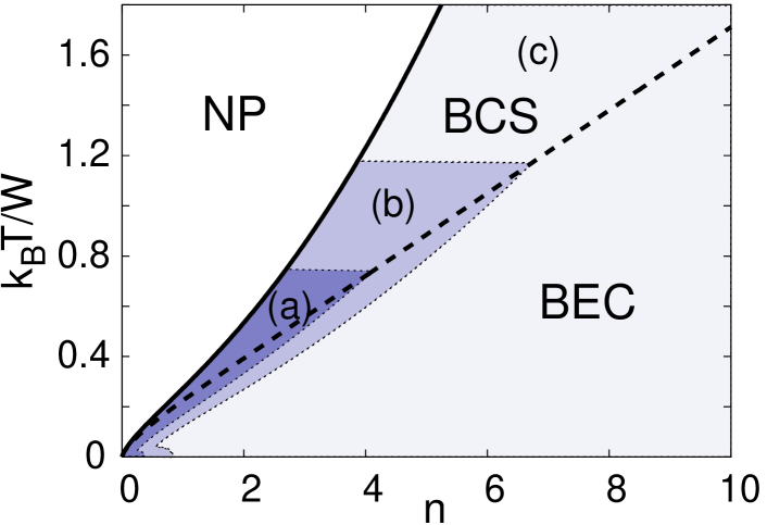
Figure 1: The diagram of the singlet phase presented in the density $n$ – temperature $T$ coordinates at $U_{0}=-0.33W$. The solid line denotes the boarder of BCS type phase with pairing (‘NP’ stands for no–pairing, normal phase), the dashed line marks the borderline of BEC quasiparticle condensate. For $U_{2}/|U_{0}|=0.59$ both phases in (c) (blank) region fulfill the standard thermodynamic stability conditions, but are unstable in (a) (grey) and (b) (light-grey) regions. For $U_{2}/|U_{0}|=0.64$ the regions (b) and (c) are thermodynamically stable, (a) region is unstable.

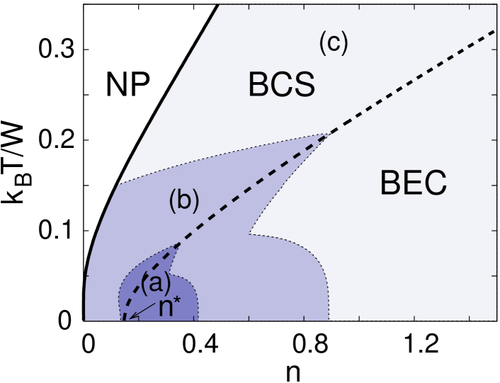
Figure 2: The diagram of the singlet phase for strong interaction $U_{0}=-W$ in the density $n$ – temperature $T$ coordinates. The zero temperature critical density is $n^{*}\approx 0.15$. The solid line denotes the border of BCS type paired phase, the dashed line marks the borderline of BEC quasiparticle condensate. Stability regions (a), (b) and (c) are defined in the same way as in Fig. 1.

In order to solve numerically Eqs. (23) and (26) we only need to provide the density of states $\rho(E)=\sum_{k}\delta(E-\xi_{k})$ in the optical lattice. We assume a simple elliptic model for the density $\rho(E)=\frac{8N_{s}}{\pi W^{2}}\sqrt{(W/2)^{2}-E^{2}}$, where $W=(32\pi)^{2/3}t$ is chosen to fit a low-energy density profile obtained from the dispersion relation $\xi_{k}$.

We are able to gain some analytical insight into the solution for this BEC singlet phase. The integrals appearing in (26) can be performed in the limit $T\rightarrow 0$ leading to

$$n =n_{\text{BEC}}+\tfrac{3}{\pi}\left[(1-\omega^{2})\arctan{\tfrac{1}{\sqrt{\omega}}}+\sqrt{\omega}(1+\omega)\right]-\tfrac{3}{2},$$ (27a)

$$-\frac{W}{U_{0}} =\frac{2n_{\text{BEC}}}{3\omega}+\tfrac{4}{\pi}\left[(1+\omega)\arctan{\tfrac{1}{\sqrt{\omega}}}-\sqrt{\omega}\right],$$ (27b)

where $\omega=\frac{2|\Delta|}{W}$. These two non-linear algebraic equations determine $n_{\text{BEC}}$ and $|\Delta|/W$ for a given $n$. We define a critical density $n^{*}$ by setting $n_{\text{BEC}}=0$ in (27). The BEC condensate solution with finite $n_{\text{BEC}}$ exists for densities larger than $n^{*}$ at $T=0$. For weak interactions $|U_{0}|/W<\frac{1}{2}$ we find only $n^{*}=0$ solution, which means that there is only the BEC phase at $T=0$. For stronger interactions $|U_{0}|/W>\frac{1}{2}$ we find a region of BCS phase extending down to zero temperature. We present the resulting finite temperature phase diagram in the weak interaction case in Fig. 1 for a fixed attractive interaction $U_{0}=-0.33W$. The situation with strong interaction is illustrated in Fig. 2 for $U_{0}=-W$. Additionally, one can obtain an analytic solution $n^{*}=\frac{32}{3\pi^{2}}|U_{0}|/W$ for $|U_{0}|/W\gg 1$.

VI Stability

We discuss below the standard thermodynamic stability conditions expressed by: i) positivity of pressure $p$, ii) positivity of constant volume specific heat $c_{V}$, and iii) positivity of isothermic compressibility $\kappa_{T}$ (for the calculation see Appendix B).

Singlet phase. We find that $c_{V}$ is positive in the singlet phase and is independent of $U_{2}$. The pressure $p$ and the inverse compressibility $\kappa_{T}^{-1}$ have a following linear dependence on $U_{2}$:

$$p(U_{0},U_{2}) =p(U_{0})+U_{2}\tfrac{5n^{2}}{9a^{3}},$$ (28a)

$$\kappa_{T}^{-1}(U_{0},U_{2}) =\kappa_{T}^{-1}(U_{0})+U_{2}\tfrac{10n^{2}}{9a^{3}}.$$ (28b)

This means that for any point on the phase diagram in Fig. 1 or Fig. 2 we can find $U_{2}$ large enough to stabilize the BCS or BEC singlet phase. The shadowed regions in these figures exemplify stability for $|U_{2}|/U_{0}=0.59$ and $0.64$, respectively.

Figure 3: The specific heat versus temperature for a fixed density $n=1.5$. The solid line illustrates the sequence of transitions for interaction strength $U_{0}=-W$, the dashed line is for $U_{0}=-0.33W$.

We illustrate the nature of subsequent transition by plotting the specific heat $c_{V}$ in Fig. 3. We show the specific heat dependence on the temperature $T$ at fixed density $n=1.5$, which is representative both for strong and weak attraction and contains all three phases: non-pairing, BCS-like and the BEC quasiparticle condensate. The plot does not depend on the strength $U_{2}$, provided it is strong enough to stabilize the phases. The specific heat exhibits a jump at the onset of pairing (marked by a triangle in Fig. 3), indicating that the corresponding transition is of second order. The transition to BEC quasiparticle condensate is contiunuos with a cusp in the specific heat dependence (marked by a square), the behaviour being known in the usual Bogoliubov theory of BEC condensation Sto99 .

We inspect further the details of stability lines shown in Fig. 2. We find generically two stable phases separated by an unstable one for the system at fixed temperature. The system will then have a tendency to spontaneously separate into the dense and dilute phases. We make this statement qualitative by considering the thermodynamic spinodal decomposition Spino95 into the dense BEC and dilute BCS or normal phase. The results are presented in Fig. 4. The spinodal stability lines are redrawn from Fig. 2, region (b). The line marked by triangles is given by the compressibility condition $\kappa_{T}^{-1}=0$, while the one marked by the squares is given by the pressure $p=0$. We find that the region denoted by light gray shadowing corresponds to a metastable state, which undergoes the spinodal dcomposition. The regions denoted BCS or BEC above the solid binodal line are stable against such a thermal fluctuation. This result indicates that the thermal fluctuations around the mean field solution do not change qualitatively our phase diagram, they are of importance at the vicinity of the stability borderlines. The role of quantum fluctuations is left for future research.

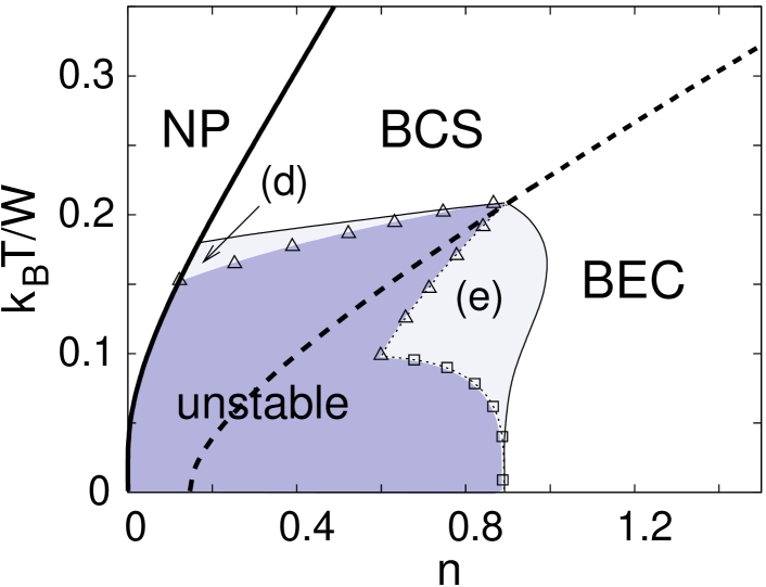
Figure 4: The phase diagram of the singlet phase with the same parameters as in Fig. 2. The binodal line is indicated by a thin solid curve. The system in both shadowed regions (d) within BCS phase and (e) within BEC phase undergoes a spinodal decomposition. The BCS phase above (d) is stable, same as BEC to the left of (e) region.

We find that the most unstable point of our diagram is located at the BCS/BEC borderline (marked by the thick dashed line in Fig. 4). We can solve the following conditions $p>0$ and $\partial p/\partial n>0$ at zero temperature on this corssover line, corresponding to the density $n^{*}$ (compare Fig. 2). We thus find $U_{2}^{c}$ – the critical strength of repulsion in the quintet channel at which the whole BCS and BEC phases become stable. In the weak interaction regime

$$U_{2}^{c}=\frac{|U_{0}|}{10}\left(2+\frac{3}{1-|U_{0}|/2W}\right),$$ (29)

which is valid for $|U_{0}|/W<\frac{1}{2}$, while in the strong interaction regime

$$U_{2}^{c}=\frac{|U_{0}|}{20}\left(1+\frac{3\,\mathrm{arctan}(1/\sqrt{\omega})}{\sqrt{\omega}-\omega\mathrm{arctan}(1/\sqrt{\omega})}\right),$$ (30)

valid for $|U_{0}|/W>\frac{1}{2}$ and with $\omega$ calculated from Eq. (27b) at $n_{\mathrm{BEC}}=0$. For the interaction strength $U_{2}>U_{2}^{c}$ there is always a non-collapsing phase, which can be either normal, BCS or BEC homogeneous, or an inhomogeneous mixture of the dilute and dense phases.

Other symetry phases. We have carried out a detailed, both analytical and numerical study of stability Pel10 for the other phases. We find that both magnetic phases $U(1)_{S_{z}-\varphi}$ and $U(1)_{S_{z}-\varphi/2}$ are mechanically unstable. The tetrahedral T-phase with the quintet pairing occurs for $U_{2}<0$ and $U_{0}>0$. It can be made thermodynamically stable by increasing the singlet repulsion $U_{0}$. We find however, that the ferromagnetic phase $U(1)_{S_{z}-\varphi}$ has lower free energy in the parameter regions, where T-phase becomes stable. Morover, we find that an infinitezimal $\epsilon>0$ distortion of T-phase order paremeter by a magnetic contribution $\Delta((1+\epsilon)\hat{C}^{2,2}+\sqrt{2}\hat{C}^{2,-1})$ leads to a lower free energy. We conclude that the T-phase is not even metastable, as it always corresponds to a saddle point of free energy.

VII Conclusions and outlook

In summary, we applied the Hartree-Fock mean-field approximation to solve a problem of pairing between bosons with spin $S=1$ moving on optical lattices. The order parameter describing such paired bosons has a matrix form. Detailed classiffiation of possible solutions according to their symmetries was presented. In particular, we found that the self-consistent equations for the $SO(3)$ symmetric phase have the same form as those for the scalar bosons. We showed that the coherent BCS type phase of paired bosons induced by attractive interaction in the singlet channel is stable provided that the interaction in a quintet channel is repulsive. This finding might be usefull in experiments to stabilize bosons with attractive interaction against mechanical collapse.

The analyzed problem might be extended in the future in different ways. For example, it would be interesting to include local quantum correlation beyond the static Hartree-Fock approximation by using the bosonic dynamical mean-field theory developed recently Byczuk08 . Another line of research is to investigate inhomogeneous excited states of bosons with $S=1$ in the BCS or BEC phases, i.e. there should be generalized vortex states in the condensed phases because of the high remaining symmetry in the system. In the boson gas with hyper spin $S=2$, where a very reach variety of spinor BEC for repulsive interactions have been proposed Die06 , we expect stabilization of at least some of many symmetry allowed phases for attractive interactions.

Appendix A Diagonalization of the mean field Hamiltonian

In this section we diagonalize our mean field Hamiltonian (7) and derive Eq. (11). We use a convenient notation Sto99 , known as the Nambu notation in the standard theory of superconductivity for fermions Bru04

$$\bm{\Phi}_{k}=(b_{k1},\,b_{k0},\,b_{k-1},\,b_{-k1}^{\dagger},\,b_{-k0}^{\dagger},\,b_{k-1}^{\dagger})^{T},$$ (31)

where the superscript $T$ denotes transposition. The bosonic canonical commutation relations rewritten with the Nambu spinor are $[(\bm{\Phi}_{k})_{\alpha},(\bm{\Phi}_{k^{\prime}}^{\dagger})_{\beta}]=(\Sigma_{z})_{\alpha\beta}\delta_{k,k^{\prime}}$ where $\alpha,\beta=1,\dots,6$ and $\Sigma_{z}={\mathrm{diag}}(\hat{\openone},-\hat{\openone})$. Here $\Sigma_{z}$ is a diagonal matrix, the symbol $\hat{\openone}$ denotes the unity $3\times 3$ matrix. We express the model Hamiltonian in the mean field approximation (7) as follows

$$H_{\text{MF}}=H^{0}+H^{\text{int}}_{\text{MF}}-\mu N=\tfrac{1}{2}\sum_{k}\bm{\Phi}^{\dagger}_{k}\Sigma_{z}M_{k}\bm{\Phi}_{k}+\mathrm{const.}.$$ (32)

The additive constant does not enter the calculation presented in this Appendix. We introduce here the $6\times 6$ matrix $M_{k}$ resulting from the commutation $[\bm{\Phi}_{k},H_{\mathrm{M}F}]=M_{k}\bm{\Phi}_{k}$. The explicit form of $M_{k}$ is given in Eq. (12).

With the Nambu spinor we write a compact expression for all normal and anomalous averages

$$\tfrac{1}{N_{s}}\sum_{\vec{k}}\left\langle\bm{\Phi}_{k}\bm{\Phi}_{k}^{\dagger}\right\rangle=\begin{pmatrix}\hat{\openone}+\hat{n}^{*}&\hat{\Lambda}\\ \hat{\Lambda}^{*}&\hat{n}\end{pmatrix},$$ (33)

where the single site occupation $\hat{n}$ and the amplitude of Cooper pair condensate $\hat{\Lambda}$ were defined in Section III. Our aim is now to compute the l.h.s. of the above equation. This is easily done with a suitable Bogoliubov transformation performed on the mean field Hamiltonian (7). We follow this route by introducing a new Nambu spinor $\bm{\Gamma}$ for quasiparticle excitations

$$\bm{\Gamma}_{k}=\begin{pmatrix}\hat{u}_{k}&\hat{v}_{k}\\ \hat{v}^{*}_{k}&\hat{u}^{*}_{k}\end{pmatrix}\bm{\Phi}_{k},$$ (34)

where $\hat{u}_{k}$ and $\hat{v}_{k}$ contain coefficients to be determined below. We require the new spinor $\bm{\Gamma}$ to describe proper quasiparticles, so $[\bm{\Gamma}_{k},H_{\text{M}F}]=E_{k}\bm{\Gamma}_{k}$, where $E_{k}={\mathrm{diag}}(\hat{e}_{k},-\hat{e}_{k})$ and $(\hat{e}_{k})_{\sigma\sigma^{\prime}}=e_{k\sigma}\delta_{\sigma\sigma^{\prime}}$. The eigenvalues $e_{k\sigma}$ correspond to the excitation energy of quasiparticles in the BCS condensate. The components of $\bm{\Gamma}_{k}$ have to fulfill the bosonic commutation relations, namely $[(\bm{\Gamma}_{k})_{\alpha},(\bm{\Gamma}_{k^{\prime}}^{\dagger})_{\beta}]=(\Sigma_{z})_{\alpha\beta}\delta_{k,k^{\prime}}$. The corresponding requirement for the coefficients of the Bogoliubov transformation (34) leads to

$$\begin{pmatrix}\hat{u}_{k}&\hat{v}_{k}\\ \hat{v}^{*}_{k}&\hat{u}^{*}_{k}\end{pmatrix}^{-1}=\Sigma_{z}\begin{pmatrix}\hat{u}_{k}&\hat{v}_{k}\\ \hat{v}^{*}_{k}&\hat{u}^{*}_{k}\end{pmatrix}^{\dagger}\Sigma_{z}.$$ (35)

Finally, we write the eigenvalue equation for the $6\times 6$ matrix $M_{k}$

$$\begin{pmatrix}\hat{u}_{k}&\hat{v}_{k}\\ \hat{v}^{*}_{k}&\hat{u}^{*}_{k}\end{pmatrix}M_{k}\begin{pmatrix}\hat{u}_{k}&\hat{v}_{k}\\ \hat{v}^{*}_{k}&\hat{u}^{*}_{k}\end{pmatrix}^{-1}=E_{k}.$$ (36)

It follows from the hermicity of $\Sigma_{z}M_{k}$ and the transformation constrain (35) that the eigenvalues of $M_{k}$ have to be real. Note also that the additional matrix $\Sigma_{z}$ enters our derivation due to the bosonic commutation relation, but is absent in the standard BCS formulation for the fermions.

It turns out that we don’t need to calculate explicitly $\hat{u}_{k}$ and $\hat{v}_{k}$ from Eq. (36) as long as we are only interested in the thermodynamic averages. The quasiparticle averages are particularly simple

$$\left\langle\bm{\Gamma}_{k}\bm{\Gamma}_{k^{\prime}}^{\dagger}\right\rangle\Sigma_{z}=(1-e^{-\beta E_{k}})^{-1}\delta_{kk^{\prime}}.$$ (37)

We transform this equation back to the original spinor $\bm{\Phi}_{k}$ with the help of Eq. (34) and we get

$$\left\langle\bm{\Phi}_{k}\bm{\Phi}_{k}^{\dagger}\right\rangle\Sigma_{z}=\begin{pmatrix}\hat{u}_{k}&\hat{v}_{k}\\ \hat{v}^{*}_{k}&\hat{u}^{*}_{k}\end{pmatrix}^{-1}(1-e^{-\beta E_{k}})^{-1}\begin{pmatrix}\hat{u}_{k}&\hat{v}_{k}\\ \hat{v}^{*}_{k}&\hat{u}^{*}_{k}\end{pmatrix},$$ (38)

which simplifies to

$$\left\langle\bm{\Phi}_{k}\bm{\Phi}_{k}^{\dagger}\right\rangle\Sigma_{z}=(1-e^{-\beta M_{k}})^{-1}.$$ (39)

The above equation together with Eq. (33) gives the final result of this Appendix.

Appendix B Calculation of thermodynamic parameters

We calculate the grand canonical potential (per site)

$$\Omega=-\tfrac{k_{B}T}{N_{s}}\ln\mathrm{Tr}e^{-\beta H_{\text{MF}}}$$ (40)

by taking the trace $\mathrm{Tr}$ over all many-particle states of second-quantized $H_{\text{MF}}$ as defined in (32). The general expression for the entropy per site $S=-\frac{\partial\Omega}{\partial T}|_{\mu}$ is then

$$S=\frac{k_{B}}{N_{s}}(\ln\mathrm{Tr}e^{-\beta H_{\text{MF}}}+\beta\left<H_{\text{MF}}\right>_{\text{MF}})$$ (41)

where $\left<\ldots\right>_{\text{MF}}$ denotes the thermodynamic average with our model mean field hamiltonian. Using the results of diagonalization of bilinear $H_{\text{MF}}$ derived in Appendix A we get

$$S=\tfrac{k_{B}}{N_{s}}\sum_{k\sigma}\left(-\ln(1-e^{-\beta e_{k\sigma}})+\frac{\beta e_{k\sigma}}{e^{\beta e_{k\sigma}}-1}\right),$$ (42)

while the constant introduced in (7) does not enter this expression. With the above explicit of $S$ we write the final compact formula for $\Omega$

$$\Omega=-TS+\tfrac{1}{N_{s}}\sum_{k}(\xi_{k}-\mu)n_{k}+E_{0},$$ (43)

where $n_{k}=\sqrt{e_{k}^{2}+|\Delta|^{2}}f(e_{k})-\tfrac{1}{2}$ is average occupation of a quasi-momentum state $k$. The constant has been now properly recovered and is entirely included in $E_{0}$ as defined in (10). For the singlet phase there is a simple scalar expression $E_{0}=\frac{3\Delta^{2}}{2U_{0}}+\frac{5U_{2}+U_{0}}{9}n^{2}$. With the grand canonical potential $\Omega$ expressed entirely in terms of the order parameter one calculates the pressure $p=-\Omega/a^{3}$, the specific heat per site $c_{V}=T\frac{\partial S}{\partial T}|_{n}$ and the inverse compressibility $\kappa_{T}^{-1}=n\frac{\partial p}{\partial n}|_{T}$.

References

- (1) L. N. Cooper, Phys. Rev 104, 1189 (1956).
- (2) J. Bardeen, L. N. Cooper, and J. R. Schrieffer, Phys. Rev. 108, 1175 (1957).
- (3) D. Jaksch and P. Zoller, Annals of Physics 315, 52 (2005).
- (4) I. Bloch, J. Dalibard, W. Zwerger, Rev. Mod. Phys. 80, 885 (2008).
- (5) A. J. Leggett, in Modern Trends in the Theory of Condensed Matter eds. A. Pekalski and R. Przystawa, pp.13-27 (Springer-Verlag, Berlin, 1980).
- (6) P. Nozieres and S. Schmitt-Rink, J. Low Temp. Phys. 59, 195 (1985).
- (7) C.A. Regal, C. Ticknor, J. L. Bohn, and D. S. Jin, Nature 424, 47 (2003).
- (8) W. A. B. Evans and Y. Imry, Nuovo Cimento 63B, 155 (1969).
- (9) W. A. B. Evans and R.I.M.A. Rashid, J. Low Temp. Phys. 11, 93 (1973).
- (10) H.T.C. Stoof, Phys. Rev. A 49, 3824 (1994).
- (11) E. Mueller and G. Baym Phys. Rev. A 62, 053605 (2000).
- (12) G. S. Jeon, L. Yin, S. W. Rhee, and D. J. Thouless, Phys. Rev. A 66, 011603, (2002).
- (13) M. Mannel, K. Morawetz, P. Lipavsky, New J. Phys. 12, 033013 (2010).
- (14) P. Zin, B. Oles, M. Trippenbach, and K. Sacha, Phys. Rev. A 78, 023620 (2008).
- (15) A. Koetsier, P. Massignan, R. A. Duine, H. T. C. Stoof, Phys. Rev. A 79, 063609 (2009).
- (16) G. Thalhammer, M. Theis, K. Winkler, R. Grimm, and J. H. Denschlag, Phys. Rev. A 71, 033403 (2005).
- (17) C. Bruder, D. Vollhardt, Phys. Rev. B 34, 131 (1986).
- (18) D. Vollhardt and P. Woelfle, The superfluid phases of Helium 3 (Taylor and Francis, London, New York, Philadelphia, 1990).
- (19) S.-K. Yip, Phys. Rev. A 75, 023625 (2007).
- (20) T. Ohmi and K. Machida, J. Phys. Soc. Jpn. 67, 1822 (1998).
- (21) T.-L. Ho, Phys. Rev. Lett. 81, 742 (1998).
- (22) M. Ueda, Y. Kawaguchi, “Spinor Bose-Einstein condensates”, preprint arXiv:1001.2072.
- (23) M. Koashi and M. Ueda, Phys. Rev. Lett. 84, 1066 (2000).
- (24) M. Ueda and M. Koashi, Phys. Rev. A. 65, 063602 (2002).
- (25) U. A. Khawaja, H. Stoof, Nature 411, 918 (2001); U. A. Khawaja, H. Stoof, Phys. Rev. A 64, 043612 (2001).
- (26) G. W. Semenoff, F. Zhou, Phys. Rev. Lett. 98, 100401 (2007).
- (27) M. P. A. Fisher, P. B. Weichman, G. Grinstein, and D. S. Fisher, Phys. Rev. B 40, 546 (1989).
- (28) D. van Oosten, P. van der Straten, and H. T. C. Stoof, Phys. Rev. A 63, 053601 (2001); Phys. Rev. A 67, 033606 (2003).
- (29) G. Mazzarella, Phys. Rev. A 73, 013625 (2006).
- (30) C. J. Pethick and H. Smith, Bose-Einstein Condensation in Dilute Gases (Cambridge University Press, Cambridge, UK, 2002).
- (31) Imambekov Phys. Rev. A 68, 063602 (2003).
- (32) H. Bruus and K. Flensberg, Many-body quantum theory in condensed matter physics: an introduction (Oxford University Press, New York, USA, 2004).
- (33) The algebraic identities and , follow from the completness of total spin basis. They are a matrix form of the ortogonality condition for the Clebsch-Gordan coefficients.
- (34) T.-L. Ho, and S.-K. Yip, Phys. Rev. Lett. 82, 247 (1999).
- (35) J. Cao, Y. Jiang, and Y. Wang, Europhys. Lett. 79, 30005 (2007).
- (36) P.M. Chaikin, T.C. Lubensky Principles of condensed matter physics (Cambridge University Press, Cambridge, UK, 1995).
- (37) G. Pełka, PhD thesis, University of Warsaw (2010), in preparation.
- (38) H.T.C. Stoof, D.B.M. Dickerscheid, and K. Gubbels, Ultracold Quantum Fields, (Springer, Netherlands 2008).
- (39) K. Byczuk and D. Vollhardt, Phys. Rev. B 77, 235106 (2008).
- (40) R.B. Diener and T.-L. Ho, Phys. Rev. Lett. 96, 190405 (2006).