Minimax risks for sparse regressions:
Ultra-high dimensional
phenomenons
Abstract
Consider the standard Gaussian linear regression model , where is a response vector and is a design matrix. Numerous work have been devoted to building efficient estimators of when is much larger than . In such a situation, a classical approach amounts to assume that is approximately sparse. This paper studies the minimax risks of estimation and testing over classes of -sparse vectors . These bounds shed light on the limitations due to high-dimensionality. The results encompass the problem of prediction (estimation of ), the inverse problem (estimation of ) and linear testing (testing ). Interestingly, an elbow effect occurs when the number of variables becomes large compared to . Indeed, the minimax risks and hypothesis separation distances blow up in this ultra-high dimensional setting. We also prove that even dimension reduction techniques cannot provide satisfying results in an ultra-high dimensional setting. Moreover, we compute the minimax risks when the variance of the noise is unknown. The knowledge of this variance is shown to play a significant role in the optimal rates of estimation and testing. All these minimax bounds provide a characterization of statistical problems that are so difficult so that no procedure can provide satisfying results.
keywords:
[class=AMS]keywords:
t11 INRA, UMR 729 MISTEA, F-34060 Montpellier, FRANCE.
1 Introduction
In many important statistical applications, including remote sensing, functional MRI and gene expressions studies the number of parameters is much larger than the number of observations. An active line of research aims at developing computationally fast procedures that also achieve the best possible statistical performances in this “ larger than ” setting. A typical example is the study of -based penalization methods for the estimation of linear regression models. However, if is really too large compared to , all these new procedures fail to achieve a good estimation.
Thus, there is a need to understand the intrinsic limitations of a statistical problem: what is the best rate of estimation or testing achievable by a procedure? Is it possible to design good procedures for arbitrarily large or are there theoretical limitations when becomes “too large”? These limitations tell us what kind of data analysis problems are too complex so that no statistical procedure is able to provide reasonable results. Furthermore, the knowledge of such limitations may drive the research towards areas where computationally efficient procedures are shown to be suboptimal.
1.1 Linear regression and statistical problems
We observe a response vector and a real design matrix of size . Consider the linear regression model
| (1.1) |
where the vector of size is unknown and the random vector
follows a centered normal distribution
. Here, stands for the null vector of
size and for the identity matrix of size .
In some cases, the design is considered as fixed either
because it has been previously chosen or because we work conditionally to
the design. In other cases,
the rows of the design matrix correspond
to a -sample of
a random vector of size . The design is then said to be
random. A specific class of random
design is made of Gaussian designs where follows a centered normal
distribution
. The analysis of fixed
and Gaussian designs share many common points. In
this work, we shall enhance the similarities and the differences between
both settings.
There are various statistical problems arising in the linear regression model (1.1). Let us list the most classical issues:
Linear hypothesis testing. In general, the aim is to test whether belongs to a linear subspace of . Here, we focus on testing the null hypothesis : . In Gaussian design, this is equivalent to testing whether is independent from .
Prediction. We focus on predicting the expectation in fixed design and the conditional expectation in Gaussian design.
Inverse problem. The primary interest lies in estimating itself and the corresponding loss function is , where is the norm in .
Support estimation aims at recovering the support of , that is the set of indices corresponding to non-zero coefficients. The easier problem of dimension reduction amounts to estimate a set of “reasonable” size that contains the support of with high probability.
Much work have been devoted to these statistical questions in the so-called high-dimensional setting, where the number of covariates is possibly much larger than . A classical approach to perform a statistical analysis in this setting is to assume that is sparse, in the sense that most of the components of are equal to . For the problem of prediction (), procedures based on complexity penalization are proved to provide good risk bounds for known variance [11] and unknown variance [6] but are computationally inefficient. In contrast, convex penalization methods such as the Lasso or the Dantzig selector are fast to compute, but only provide good performances under restrictive assumptions on the design (e.g. [8, 13, 50]). Exponential weighted aggregation methods [18, 40] are another example of fast and efficient methods. The penalization methods have also been analyzed for the inverse problem () [8] and for support estimation () [36, 49]. Dimension reduction methods are often studied in more general settings than linear regression [17, 26]. In the linear regression model, the SIS method [25] based on the correlation between the response and the covariates allows to perform dimension reduction. The problem of high-dimensional hypothesis testing () has so far attracted less attention. Some testing procedures are discussed in [7, 3] for fixed design and in [44, 34] for Gaussian design.
1.2 Sparsity and ultra-high dimensionality
Given a positive
integer , we say that the
vector is -sparse if contains at most non-zero
components. We call the sparsity parameter. In this paper, we are interested
in the setting .
We note the set of -sparse vectors in
.
In linear regression, most of the results about classical procedures require that the triplet satisfies . When is “small”, this corresponds to assuming that is subexponential with respect to . The analysis of the Lasso in prediction, inverse problems [8], and support estimation [38] entail such assumptions. In dimension reduction, the SIS method [25] also requires this assumption. If the multiple testing procedure of [7] can be analyzed for larger than , it exhibits a much slower rate of testing in this case. In noiseless problems (), compressed sensing methods [23] fail when is large compared to (see [22] for numerical illustrations). In the sequel, we say that the problem is ultra-high dimensional111In some papers, the expression ultra-high dimensional has been used to characterize problems such that with . We argue in this paper that that as soon as goes to , the case is not intrinsically more difficult than conditions such as with . when is large compared to . Observe that ultra-high dimensionality does not necessarily imply that is exponential with respect to . As an example, taking and asymptotically yields an ultra-high dimensional problem.
Why should we care about ultra-high dimensional problem? In this setting, there are so many variables that statistical questions such as the estimation of () or its support () are likely to be difficult. Nevertheless, if the signal over noise ratio is large, do there exist estimators that perform relatively well? The answer is no. We prove in this paper that a phase transition phenomenon occurs in an ultra-high dimensional setting and that most of the estimation and testing problems become hopeless. This phase transition phenomenon implies that some statistical problems that are tackled in postgenomic of functional MRI cannot actually be addressed properly.
Example 1.1 (Motivating example).
In some gene network inference problems (e.g. [16]), the number of genes can be as large as 5000 while the number of microarray experiments is only of order 50. Let us consider a gene . We note the set of genes that interact with the gene and stands for the cardinality of . How large can be so that it is still “reasonable” to estimate from the microarray experiments? In statistical terms, inferring the set of genes interacting with amounts to estimate the support of a vector in a linear regression model (see e.g. [38]). Our answer is that if is larger than , then the problem of network estimation becomes extremely difficult. We will come back to this example and explain this answer in Section 7.
1.3 Minimax risks
A classical way to assess the performance of an estimator is to consider its maximal risk over a class . This is the minimax point of view. For the time being, we only define the notions of minimaxity for estimation problems ( and ). Their counterpart in the case of testing () and dimension reduction () will be introduced in subsequent sections. Given a loss function and estimator , the maximal risk of over for a design (or a covariance in the Gaussian design case) and a variance is defined by . Taking the infimum of the maximal risk over all possible estimators , we obtain the minimax risk
We say that an estimator
is minimax if its maximal risk over is close to the minimax risk.
In practice, we do not know the number of non-zero components of and we seldom know the variance of the error. If an estimator does not require the knowledge of and nearly achieves the minimax risk over for a range of , we say that is adaptive to the sparsity. Similarly, an estimator is adaptive to the variance , if it does not require the knowledge of and nearly achieves the minimax risk for all . When possible, the main challenge is to build adaptive procedures. In some statistical problems considered here, adaptation is in fact impossible and there is an unavoidable loss when the variance or the sparsity parameter is unknown. In such situations, it is interesting to quantify this unavoidable loss.
1.4 Our contribution and related work
In the specific case of the Gaussian sequence model, where and , the minimax risks over -sparse vectors have been studied for a long time. Donoho and Johnstone [21, 35] have provided the asymptotic minimax risks of prediction . Baraud [5] has studied the optimal rate of testing from a non-asymptotic point of view while Ingster [31, 32, 33] has provided the asymptotic optimal rate of testing with exact constants.
Recently, some high-dimensional problems have been studied from a minimax point of view. Wainwright [45, 46] provides minimax lower bounds for the problem of support estimation (). Raskutti et al. [39] and Rigollet and Tsybakov [40] have provided minimax upper bounds and lower bounds for and over balls for general fixed designs when the variance is known (see also Ye and Zhang [47] and Abramovich and Grinshtein [1]). Arias-Castro et al. [3] and Ingster et al. [34] have computed the asymptotic minimax detection boundaries for the testing problem for some specific designs. However, their study only encompasses reasonable dimensional problems ( grows polynomially with ). Some minimax lower bounds have also been stated for testing () and prediction () problems with Gaussian design [42, 44]. All the aforementioned results do not cover the ultra-high dimensional case and do not tackle the problem of adaptation to both and .
This paper provides minimax lower bounds and upper bounds for the problems (), (), () when the regression vector is -sparse for fixed and random designs, known and unknown variance, known and unknown sparsities. The lower and upper bounds match up to possible differences in the logarithmic terms. The main discoveries are the following:
-
1.
Phase transition in an ultra-high dimensional setting. Contrary to previous work, our results cover both the high-dimensional and ultra-high dimensional setting. We establish that for each of the problems (), () and (), an elbow effect occurs when becomes large compared to . Let us emphasize the difference between the high-dimensional and the ultra-high dimensional regimes for two problems: prediction () and support estimation ().
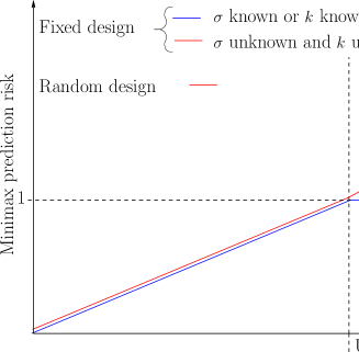
Prediction with random design. In the (non-ultra) high-dimensional setting, the minimax risk of prediction for a random design regression is of order (see Section 3). Thus, the effect of the sparsity is linear and the effect of the number of variables is logarithmic. In an ultra-high dimensional setting, that is when is large, we establish that an elbow effect occurs in the minimax risk. In this setting, the minimax risk becomes of order , where is a positive constant : it grows exponentially fast with and polynomially with (see the red curve in Figure 1). If it was expected that the minimax risk cannot be small for such problems, we prove here that the minimax risk is in fact exponentially larger than the usual term.
Support estimation. In a non-ultra high dimensional setting it is known [46] that under some assumptions on the design (e.g. each component of is drawn from iid. standard normal distribution) the support of a -sparse vector is recoverable with high probability if
(1.2) where is a numerical constant. In an ultra-high dimensional setting, even if
(1.3) it is not possible to estimate the support of with high probability. Observe that the condition (1.3) is much stronger than (1.2). In fact, it is not even possible to reduce drastically the dimension of the problem without forgetting relevant variables with positive probability. More precisely, for any dimension reduction procedure that selects a subset of variables of size with some (described in Proposition 6.7), we have with probability away from zero (see Proposition 6.7). Thus, it is almost hopeless to have a reliable estimation of the support of even if is large. This impossibility of dimension reduction for ultra-high dimensional problems is numerically illustrated in Section 7.
-
2.
Adaptation to the sparsity and to the variance . Most theoretical results for the problems () and () require that the variance is known. Here, we establish these minimax bounds for both known and unknown variance and known and unknown sparsity. The knowledge of the variance is proved to play a fundamental role for the testing problem () when is large compared to . The knowledge of is also proved to be crucial for () in an ultra-high dimensional setting. Thus, specific work is needed to develop fast and efficient procedures that do not require the knowledge of the variance. Furthermore, variance estimation is extremely difficult in an ultra-high dimensional setting.
-
3.
Effect of the design. Lastly, the minimax bounds of , and are established for fixed and Gaussian designs. Except for the problem of prediction , the minimax risks are shown to be of the same nature for both forms of the design. Furthermore, we investigate the dependency of the minimax risks on the design (resp. ) in Sections 4-6.
The minimax bounds stated in this paper are non asymptotic. While some upper bounds are consequences of recent results in the literature, most of the effort is spent here to derive the lower bound. These bounds rely on Fano’s and Le Cam’s methods [48] and on geometric considerations. In each case, near optimal procedures are exhibited.
1.5 Organization of the paper
In Section 3, we summarize the minimax bounds for specific designs called “worst-case” and “best-case” designs in order to emphasize the effects of dimensionality. The general results are stated in Section 4 for the tests and Section 5 for the problem of prediction. The problems of inverse estimation, support estimation, and dimension reduction are studied in Section 6. In Section 7, we address the following practical question: For exactly what range of should we consider a statistical problem as ultra-high dimensional? A small simulation study illustrates this answer. Section 8 contains the final discussion and side results about variance estimation. Section 9 is devoted to the proof of the mains minimax lower bounds. Specific statistical procedures allow to establish the minimax upper bounds. Most of these procedures are used as theoretical tools but should not be applied in a high dimensional setting because they are computationally inefficient. In order to clarify the statements of the results in Sections 4–6, we postpone the definition of these procedures to Section 10. The remaining proofs are described in a technical appendix [43].
2 Notations and preliminaries
We respectively note and the norms in and , while refers to the inner product in . For any and , and refer to the joint distribution of . When there is no risk of confusion, we simply write and . All references with a capital letter such as Section A or Eq.(A.3) refer to the technical Appendix [43].
In the sequel, we note
the support of . For any ,
stands for the collections of all
subsets of with cardinality . Given , we note the vector of size corresponding to -th column of .
For , stands for the submatrix of that contains the columns , .
In what follows, we note the transposed matrix of .
Gaussian design and conditional distribution. When the design is said to be “Gaussian”, the rows of are independent samples of a random row vector such that . Thus, if a -sample of the random vector , where is defined by
| (2.1) |
where . The linear regression model with
Gaussian design is relevant to understand the conditional distribution of
a Gaussian variable conditionally to a Gaussian vector since
and . This is why we shall often
refer to as the conditional variance of when considering
Gaussian design. This model is also closely
connected to the estimation of Gaussian graphical
models [38, 44].
As explained later, the minimax risk over strongly depends on the design . This is why we introduce some relevant quantities on .
Definition 2.1.
Consider some integer and some design .
| (2.2) |
In fact, and respectively correspond to the largest and the smallest restricted eigenvalue of order of .
Given a symmetric real square matrix , stands for the largest eigenvalue of . Finally, , , denote positive universal constants that may vary from line to line. The notation specifies the dependency on some quantities.
In the propositions, the constants involved in the assumptions are not always expressly specified. For instance, sentences of the form “Assume that . Then, ” mean that “There exists an universal such that if , then ”.
3 Main results
The exact bounds are stated in Section 4–6. In order to explain these results, we now summarize the main minimax bounds by focusing on the role of rather than on the dependency on the design . In order to keep the notations short, we do not provide in this section the minimal assumptions of the results. Let us simply mention that all of them are valid if the sparsity satisfies and that where a positive numerical constant.
3.1 Prediction
3.1.1 Definitions
First, the results are described for the problem of prediction () since the problem of minimax estimation is more classical in this setting. Different prediction loss functions are used for fixed and Gaussian designs. When the design is considered as fixed, we study the loss . For Gaussian design, we consider the integrated prediction loss function:
| (3.1) |
Given a design , the minimax risk of prediction over with respect to is
| (3.2) |
For a Gaussian design with covariance , we study the quantity
| (3.3) |
These minimax risks of prediction do not only depend on but also on the design (or on the covariance ). The computation of the exact dependency of the minimax risks on or is a challenging question. To simplify the presentation in this section, we only describe the minimax prediction risks for worst-case designs defined by
| (3.4) |
the supremum being taken over all designs of size (resp. all covariance matrices ). The quantity corresponds to the smallest risk achievable uniformly over and all designs . It is shown in Section 5 that the quantity is achieved (up to constants) for a covariance while the quantity is achieved with high probability for designs that are realizations of the standard Gaussian design (all the components of are drawn independently from a standard normal distribution). This corresponds to designs used in compressed sensing [23]. In fact, the maximal risks and for the prediction problem correspond to typical situations where the designs is well-balanced, that is as close as possible to orthogonality.
3.1.2 Results
In the sequel, we say that is of order , where is positive constant when there exist two positive universal constants and such that
These minimax risks are computed in Section 5 and are gathered in Table 1. They are also depicted on Figure 1.
| Fixed Design: | Gaussian Design: |
|---|---|
When remains small compared to , the minimax risk of
prediction is of the same order for fixed and Gaussian design. The
risk is classical
and has been known for a long time in the specific case of the Gaussian sequence
model [35]. Some procedures based on complexity
penalization or aggregation (e.g. [11]) are
proved to achieve these risks uniformly over all designs .
Computationally efficient procedures like the Lasso or the Dantzig selector
are only proved to achieve a risk under assumption on the design [8]. If the support of is known in advance, the
parametric risk is of order . Thus, the price to pay for
not knowing the support of is only logarithmic in .
In an ultra-high dimensional setting, the minimax prediction risk in fixed
designs remains smaller than one. It is the minimax risk of estimation of the
vector of size . This means that the sparsity index
does not play anymore a role in ultra-high dimension. For a Gaussian design,
the minimax prediction risk becomes of order : it increases
exponentially fast with respect to and polynomially fast with respect to .
Comparing this risk with the parametric rate , we observe that the price to
pay for not knowing
the support of is now far higher than .
In Section 5, we also study the adaptation to the sparsity index and to the variance . We prove that adaptation to and is possible for a Gaussian design. In fixed design, no procedure can be simultaneously adaptive to the sparsity and the variance (see the red curve in Figure 1 that corresponds to fixed design, and unknown).
3.2 Testing
3.2.1 Definitions
Let us turn to the problem of testing : against : . We fix a level and a type II error probability . Minimax lower and upper bounds for this problem are discussed in Section 4.
Suppose we are given a test procedure of level for fixed design and known variance . The -separation distance of over , noted is the minimal number , such that rejects with probability larger than if . Hence, corresponds to the minimal distance such that the hypotheses and , are well separated by the test .
Although the separation distance also depends on , , and , we only write for the sake of conciseness. By definition, the test has a power larger than for such that . Then, we consider
| (3.5) |
The infimum runs over all level- tests. We call this quantity the -minimax separation distance over with design and variance . The minimax separation distance is a non-asymptotic counterpart of the detection boundaries studied in the Gaussian sequence model [20].
Similarly, we define the -minimax separation distance over with Gaussian design by replacing the distance by the distance :
| (3.6) |
Various bounds on , are stated in Section 4. In this section, we only provide the orders of magnitude of the minimax separation distances in the “worst case” designs in order to emphasize the effect of dimensionality:
| (3.7) |
This is the smallest separation distance that can be achieved by a procedure uniformly over all designs (resp. ). As for the prediction problem, it will be proved in Section 4, that the quantity and are achieved for well-balanced designs.
It is not always possible to achieve the minimax separation distances with a procedure that does not require the knowledge of the variance . This is why we also consider and the minimax separation distance for fixed and Gaussian design when the variance is unknown. Roughly, corresponds to the minimal distances that allows to separate well the hypotheses and when is unknown. We shall provide a formal definition at the beginning of Section 4.
3.2.2 Results
In Table 2, we provide the orders of the minimax separation distances over for fixed and Gaussian designs, known and unknown variance (see also Figure 2).
| Fixed and Gaussian Design | |
|---|---|
| Known : and | |
| Unknown : and |
In contrast to , the minimax separation distances are of the same order for fixed and Gaussian design.
- 1.
-
2.
When , the minimax separation distances are different under known and unknown variance. If the variance is known, the minimax separation distance over stays of order . Here, corresponds in fixed design to the minimax separation distance of the hypotheses against the general hypothesis for known variance (see Baraud [5]).
-
3.
If the variance is unknown, the minimax separation distance over is still of order if is small compared to . In contrast, the minimax separation distance blows up to the order in a ultra-high dimensional setting. This blow up phenomenon has also been observed in the previous section for the problem of prediction in Gaussian design. In conclusion, the knowledge of the variance is of great importance for larger than .
3.3 Inverse problem and support estimation
3.3.1 Definitions
In the inverse problem (), we are primarily interested in the estimation of rather than . This is why the loss function under study is . Minimax lower and upper bounds for this loss function are discussed in Section 6. For a fixed design , the minimax risk of estimation is
| (3.8) |
If one transforms the design by an homothety of factor , then this multiplies the minimax risk for the inverse problem by a factor . For the sake of simplicity, we restrict ourselves to designs such that each column has been normed to . The collection of such designs is noted . The supremum of the minimax risks over the designs is . Take for instance a design where the two first columns are equal. In this section, we only present the infimum of the minimax risks over as varies across :
The quantity is interpreted the following way: given
what is the
smallest risk we can hope if we use the best possible design? Alternatively, given observations, what is the intrinsic difficulty of estimating a -sparse vector of size ?
We call this quantity the minimax risks for the inverse problem over
.
In Section 6, we also study the corresponding the minimax risks of the inverse problem in the random design case. Let stand for the set of covariance matrices that contain only ones on the diagonal. We respectively define the minimax risk of estimation over for a covariance and the minimax risk of estimation over as
| (3.9) |
3.3.2 Results
In Table 3, we provide the minimax risks in fixed design for different values of (see also Figure 3).
| Minimax risk | . |
|---|
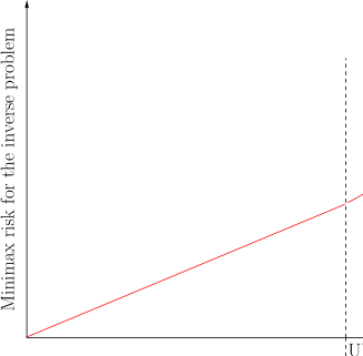
If remains smaller than , it is possible to recover
the risk for “good” designs. This risk is for instance
achieved by the Dantzig
selector of Candès and Tao [15] for nearly-orthogonal designs,
that roughly means that the restricted eigenvalues and
of are close
to one. In an ultra high-dimensional setting, it is not anymore
possible to build nearly-orthogonal designs and the minimax risk of
the inverse
problem blows up as for testing problems () or prediction problems
in Gaussian design (). Moreover, adaptation to the sparsity and to the variance is possible for the inverse problem.
As explained in Section 6, the quantities and behave somewhat similarly to their fixed design counterpart.
In Section 6, we also discuss the consequences of the minimax bounds on the problem of support estimation (). We prove that, in an ultra-high dimensional setting, it is not possible to estimate with high probability the support of unless the ratio is larger than . In fact, even the problems of support estimation is almost hopeless in an ultra-high dimensional setting.
4 Hypothesis Testing
We start by the testing problem () because some minimax lower bounds in prediction and inverse estimation derive from testing considerations.
4.1 Known variance
4.1.1 Gaussian design
As mentioned in the introduction, the knowledge of is really unlikely in many practical applications. Nevertheless, we study this case to enhance the differences between known and unknown conditional variances. Furthermore, these results turn out to be useful for analyzing the minimax separation distances in fixed design problems. We recall that the notions of minimax separation distances , , , and have been defined in Section 3.2.
Theorem 4.1.
Remark 4.1.
[Adaptation to sparsity] It follows from Theorem 4.1 that adaptation to the sparsity is possible and that the optimal optimal separation distance is of order
| (4.3) |
for all sparsities between and .
Remark 4.2.
[Correlated design] The upper bound (4.2) is valid for any covariance matrix . In contrast, the minimax lower bound (4.1) is restricted to the case . This implies that there exists some constant such that ,
In other words, the testing problem is more complex (up to constants) for an independent design than for a correlated design.
Remark 4.3.
[Which logarithmic term in the bound: or ?] In the proof of Theorem 4.1, we derive the following bounds
These two bounds are of order of (4.3) as it is assumed that . However, the dependency of the logarithmic terms on in the last bounds do not allow to provide the minimax separation distance when and is close to . For instance, if and , the two bounds only match up to a factor . The non-asymptotic minimax bounds of Baraud [5] in the Gaussian sequence model suffer the same weakness. Up to our knowledge the dependency on of the minimax separation distances has only been captured in an asymptotic setting [3, 34] ().
4.1.2 Fixed design
The separation distances are similar to the Gaussian design case.
Theorem 4.2.
Assume that , , and that . For any , there exist some designs such that
| (4.4) |
For any and any design , we have
| (4.5) |
Furthermore, this upper bound is simultaneously achieved for all and by a procedure (defined in Section 10.1.1).
As for the random design case, we conclude that adaptation to the sparsity is possible and that is of order . In fact, the proof shows that, with large probability, designs whose components are independently sampled from a standard normal variable satisfy (4.4).
Arias-Castro et al. [3] and Ingster et al. [34] have recently provided the asymptotic minimax separation distance with exact constant for known variance when the design satisfies very specific conditions. Theorem 4.2 provides the non-asymptotic counterpart of their result, but the constants in (4.4) and (4.5) are not optimal.
4.2 Unknown variance
4.2.1 Preliminaries
We now turn to the study of the minimax separation distances when the variance is unknown. In Section 3.2, we have introduced the notions of -separation distances and -minimax separation distances when the variance . We now define their counterpart for an unknown variance .
Let us consider a test of the hypothesis for the linear regression model with fixed design . We say that has a level under unknown variance if
This means that the type I error probability is controlled uniformly over all variance . Similarly, we want to control the type II error probabilities uniformly over all variances. The -separation distance of over for unknown variance is defined by
| (4.8) |
Hence, corresponds to the minimal distance such that the hypotheses and are well separated by the test . Taking the infimum over all level tests, we get the minimax separation distance over with design and unknown variance is
| (4.9) |
Finally, corresponds to the -minimax separation distance over with the “worst-case designs”.
4.2.2 Gaussian design
Minimax bounds have been proved in [44] in the non ultra-high dimensional setting. The next theorem encompasses high dimensional and ultra-high dimensional settings.
Theorem 4.3.
Suppose that and that . For any , the -minimax separation distance over with covariance and unknown variance satisfies
| (4.10) |
For any and any covariance , we have
| (4.11) |
Furthermore, this upper bound is simultaneously achieved for all and by a procedure (defined in Section 10.1.2).
Remark 4.4.
[Minimax adaptation] It follows from Theorem 4.3 that, under unknown variance, adaptation to the sparsity is possible and that the minimax separation distance over is of order
| (4.12) |
Remark 4.5.
The condition can be replaced by with , the only difference being that the constants involved in (4.10) would depend on . These conditions are not really restrictive for a sparse high-dimensional regression since the usual setting is .
Note implies that so that we cannot distinguish terms from or . As a consequence (4.12) does not necessarily capture the right dependency on in the logarithmic terms. This observation also holds for all the next results that require .
Remark 4.6.
[Dependent design] As for the known variance case, we have , that is the testing problem is more complex for an independent design than for a correlated design. For some covariance matrices , the minimax separation distance with covariance is much smaller than . Verzelen and Villers [44] provide such an example of a matrix in (see Propositions 8 and 9). However, the arguments used in the proof of their example are not generalizable to other covariances. In fact, the computation of sharp minimax bounds that capture the dependency of on remains an open problem.
4.2.3 Fixed design
Ingster et al. [34] derive the asymptotic minimax separation distance for some specific design when goes to . Here, we provide the non asymptotic counterpart that encompass all the regimes.
Proposition 4.4.
Assume that and that . For any , there exist some designs such that
| (4.13) |
For any and any design , we have
| (4.14) |
Furthermore, this upper bound is simultaneously achieved for all and by a procedure (defined in Section 10.1.2).
Again, we observe a phenomenon analogous to the random design case.
4.3 Comparison between known and unknown variance
There are three regimes depending on . They are depicted on Figure 2:
-
1.
. The minimax separation distances are of the same order for known and unknown . The minimax distance is also of the same order as the minimax risk of prediction.
-
2.
. If is known, the minimax separation distance is always of order . In such a case, an optimal procedure amounts to test the hypothesis against using the statistic . If is unknown, the statistic is not available and the minimax separation distance behaves like .
-
3.
. If is unknown, the minimax separation distance blows up. It is of order . Consequently, the problem of testing becomes extremely difficult in this setting.
5 Prediction
In contrast to the testing problem, the minimax risks of prediction () exhibit really different behaviors in fixed and in random design. The big picture is summarized in Figure 1. We recall that the minimax risks , , , and are defined in Section 3.1.
5.1 Gaussian design
Proposition 5.1.
[Minimax lower bound for prediction] Assume that . For any , we have
| (5.1) |
Remark 5.1.
[General covariances ] The lower bound (5.1) is only stated for the identity covariance . For general covariance matrices , we have
| (5.2) |
for any . This statement has been proved in [42] (Proposition 4.5) in the special case of restricted isometry, but the proof straightforwardly extends to restricted eigenvalue conditions. For , the lower bound (5.2) does not capture the elbow effect in an ultra-high dimensional setting (compare with (5.1)).
Theorem 5.2.
[Minimax upper bound] Assume that . There exists an estimator (defined in Section 10.2.1) such that the following holds:
-
1.
The computation of does not require the knowledge of or .
-
2.
For any covariance , any , any , and any we have
(5.3)
In contrast to similar results such as Theorem 1 in Giraud [27] or Theorem 3.4 in Verzelen [42], we do not restrict to be smaller than , that is we encompass both high-dimensional and ultra-high dimensional setting. The proof of the theorem is based on a new deviation inequality for the spectrum of Wishart matrices stated in Lemma 11.2.
Remark 5.2.
Remark 5.3.
[Adaptation to sparsity and the variance] The estimator does not requires the knowledge of and of the variance . It follows that is minimax adaptive to all and to all . As a consequence, adaptation to the sparsity and to the variance is possible for this problem.
Remark 5.4.
[Dependent design] The risk upper bound of stated in Theorem 5.2 is valid for any covariance matrix of the covariance . In contrast, the minimax lower bound of Theorem 4.3 is restricted to the identity covariance. This implies that the minimax prediction risk for a general matrix is at worst of the same order as in the independent case: there exists a universal constant such that for all covariance ,
In Remark 5.1, we have stated a minimax lower bound for prediction that depends on the restricted eigenvalues of . Fix some . If we consider some covariance matrices such that , the minimax lower bound (5.2) and the upper bound (5.3) match up to a constant . In general, the lower bound (5.2) and the upper bound (5.3) do not exhibit the same dependency with respect to , especially when is close to zero.
5.2 Fixed design
5.2.1 Known variance
The minimax prediction risk with known variance has been studied in Raskutti et al. [39] and Rigollet and Tsybakov [40] (see also [1, 47]). For any design and any , these authors have proved that the minimax risk satisfies
| (5.4) |
Next, we bound the supremum and we study the possibility of adaptation to the sparsity.
Proposition 5.3.
For any , the supremum is lower bounded as follows
| (5.5) |
Assume that . There exists an estimator (defined in Section 10.2.2) which satisfies
| (5.6) |
for any .
Remark 5.5.
If is small compared to , the minimax risk is of order . In an ultra-high dimensional setting, this minimax risk remains close to one. This corresponds (up to renormalization) to the minimax risk of estimation of the vector of size . As a consequence, the sparsity assumption does not play anymore a role in a ultra-high dimensional setting. From (5.6), we derive that adaptation to the sparsity is possible when the variance is known.
Remark 5.6.
[Dependency of on ] For designs , such that the ratio is close to one, the lower bounds and upper bounds of (5.4) agree with each other. This is for instance the case of the realizations (with high probability) of a Gaussian standard independent design (see the proof of Proposition 5.3 for more details).
Remark 5.7.
[Comparison with procedures] The designs for which procedures such as the Lasso or the Dantzig selector are proved to perform well require that is close to one. It is interesting to notice that these designs precisely correspond to situations where the minimax risk is close to its maximum (see Equation (5.4)). We refer to [39] for a more complete discussion.
Remark 5.8.
Proof.
If , then
.
We also have
. The last inequality follows from the risk of an estimator .
Gathering these two bounds allows to conclude.
∎
5.2.2 Unknown variance
We now consider the problem of prediction when the variance is unknown.
Proposition 5.4.
For any , there exists an estimator that does not require the knowledge of such that
| (5.7) |
Thus, the optimal risk of prediction over remains of the same order for known and unknown .
Let us now study to what extent adaptation to the sparsity is possible when the variance is unknown. In order to get some ideas let us provide risk bounds for two procedures that do not require the knowledge of : the estimator already studied for Gaussian design (defined in Section 10.2.1) and the estimator defined by .
Proposition 5.5.
[Risk bound for and ] Assume that . For any , the maximal risk of over is upper bounded as follows
| (5.8) |
For any , the maximal risk of over is upper bounded as follows
| (5.9) |
The risk bound (5.8) is also satisfied by the procedure of Baraud et al. [6]. The proof of (5.8) is a consequence of one of their results.
Remark 5.9.
As a consequence, simultaneously achieves the minimax risk over all for all such that . In an ultra-high dimensional setting, the maximum risk of over is controlled by while the minimax risk is smaller than . If the upper bound (5.8) is sharp then this would imply that is not adaptive to the sparsity in an ultra-high dimensional setting.
In contrast, is minimax adaptive over all such that , but its behavior is suboptimal in a non-ultra-high dimensional setting.
In order to get an estimator that is adaptive to all indexes , we would need to merge the properties of (for non-ultra-high dimensional cases) and of (for ultra-high dimensional cases). The following proposition tells us that it is in fact impossible.
Proposition 5.6.
[Adaptation to the sparsity is impossible under unknown variance] Consider any and such that . There exists a design of size such that for any estimator , we have either
As a benchmark, we recall the minimax upper bounds:
The proof of proposition 5.6 is based on the minimax lower bounds (4.13) for the testing problem () under unknown variance. The proof uses designs that are realizations of standard Gaussian designs.
Remark 5.10.
In the setup of Proposition 5.6, any estimator that does not require the knowledge of and has to pay at least one of these two prices:
-
1.
The estimator does not use the sparsity of the true parameter . Its risk for estimating is of the same order as the minimax risk over . The estimator has this drawback.
-
2.
For any , we have
This is the price for adaptation when is unknown. The estimator exhibits this behavior.
As a conclusion, it is impossible to merge the qualities of and of .
The best prediction risk that can be achieved by a procedure that aim to adaptation to the sparsity is of order
In other words, the unavoidable loss for adaptation for unknown variance is a factor In this sense, the estimator (and as a byproduct the procedure of Baraud et al. [6]) achieves the optimal prediction risk under unknown variance and unknown sparsity.
In conclusion, the minimax risks of prediction are of the same order for fixed and Gaussian design and for known and unknown variance when is small compared to . In an ultra-high dimensional setting, the minimax risks behave differently. For Gaussian design, the minimax risk is of the order . In contrast, the minimax risk of prediction remains smaller than one for fixed design regression with known variance. When the sparsity and the variance are unknown, there is a price to pay for adaptation under fixed design. All these behaviors are depicted on Figure 1.
6 Inverse problem and support estimation
6.1 Minimax risk of estimation
We recall that the minimax risks of estimation for the inverse problem , , , and have been defined in Section 3.3.
6.1.1 Fixed design
First, we consider the problem () for a fixed design regression model. The minimax risk of estimation over with a design is noted and is defined in (3.8). Raskutti et al. [39] have recently provided the following bounds
| (6.1) |
that holds for any fixed design and any . The lower and upper bounds match up to the factor . The upper bound is achieved by least-squares estimator over [39]. If the restricted eigenvalues of are close to one, then the minimax risk is of order . Next, we improve the lower bound in (6.1) in order to grasp the behavior of the minimax risk for non orthogonal design.
Proposition 6.1.
For any design and any , we have
| (6.2) |
In order to interpret these bounds let us restrict ourselves to design such that each column has norm, as justified in Section 3.3. The collection of such designs is noted . Observe that enforces .
In the sequel, we are interested in the smallest minimax risk that is achievable if we can choose the design , that is we want to bound . The minimax risk tells us the intrinsic difficulty of estimating a sparse vector of size with observations.
Proposition 6.2.
-
1.
Assume that . Then, we have
(6.3) This bound is for instance achieved for designs that are realizations (with a high probability) of normalized standard Gaussian design.
-
2.
For any design and any , we have
(6.4) -
3.
For any , we have
(6.5)
Remark 6.1.
The bound (6.3) tells us that the best minimax risk that is achievable in a non-ultra-high dimensional setting is of order . The Lasso achieves the (almost optimal) risk bound under some assumptions on the design matrix.
Remark 6.2.
The lower bound (6.4) is of geometric nature. Combined with (6.2), it implies the lower bound of (6.5). In an ultra-high dimensional setting, it is not possible to build a design such that is close to one (see Remark 5.8). In fact, the quantity blows up because of geometric constrains. When is larger compared to , both bounds in (6.5) are comparable and the minimax risk is of order . As a consequence, the inverse problem becomes extremely difficult in an ultra-high dimensional setting.
Remark 6.3.
While the quantity in (6.3) is due to the “size” of the parameter space , the exponential term of the minimax risk in ultra-high dimension is essentially driven by geometrical constrains on the design .
Proposition 6.3 (Adaptation to the sparsity and the variance).
As in the prediction case, we consider the estimator (defined in Section 10.2.1). Assume that . For any design , any , any , and any , we have
| (6.6) |
with probability larger than .
Remark 6.4.
Although the bound (6.6) is in probability and not in expectation, it suggests that adaptation to the sparsity and to the variance are possible.
6.1.2 Random design
Let us turn to the Gaussian design case. We are interested in bounding and as defined in (3.9).
Proposition 6.4.
For any , and any covariance we have
| (6.7) |
As long as , we derive that satisfies
| (6.8) |
We observe that and behave similarly in a non-ultra-high dimensional setting.
Remark 6.5.
[Ultra-high dimensional case] Proposition 6.4 does not allow to derive the order of magnitude of in an ultra-high dimensional setting. While the upper bound in (6.7) is blowing up, the lower bound remains as small as . Nevertheless, we know from Proposition 5.1 that
This suggests that is blowing up in an ultra-high dimensional setting but the problem remains open.
In the next proposition, we state the counterpart of Proposition 6.3 in the random design case.
Proposition 6.5 (Adaptation to the sparsity and the variance).
As in the prediction case, we consider the estimator (defined in Section 10.2.1). Assume that . For any covariance , any , any , and any , we have
| (6.9) |
with probability larger than .
6.2 Consequences on support estimation
We deduce from the minimax lower bounds for the inverse problem some consequences for the support estimation problem in a ultra-high dimensional setting. The case small compared to has been studied in Wainwright [45].
Definition 6.1.
For any and any , the set is made of all vectors in such that contains exactly non-zero coefficients that are all equal to .
In a non-ultra high dimensional setting, Wainwright [46] has proved, that under suitable conditions on a design , it is possible to recover the support of any vector that belong to with of order of . Here, we prove that has to be much larger in an ultra-high dimensional setting.
Proposition 6.6.
[Support recovery is almost impossible] For any and any , we have
For any design it is not possible to recover the support of with high probability, unless satisfies:
This quantity is blowing up in an ultra-high dimensional setting and it can be much larger than the usual that can be achieved in a non-ultra high dimensional setting.
As it is almost impossible to estimate the support of in an ultra-high dimensional setting, we may aim to an easier objective. Can we choose a subset of of size that contains the support of with high probability? This would allow to reduce the dimension of the problem from to . Dimension reductions techniques are popular for analyzing high dimensional problems. We study here to what extent dimension reduction is a realistic objective: how large should be the non-zero components of ? How small can we choose ?
Proposition 6.7.
Consider a Gaussian design regression with and . We assume that and . Set
There exists a universal constant such that for any measurable subset of of size , we have
| (6.10) |
In an ultra-high dimensional setting, it is therefore not possible to reduce the dimension of the problem to unless the square norm of is of order . In (6.10), the number is of no particular significance. It can be replaced by any constant if we take an asymptotic point of view ().
Remark 6.6.
Remark 6.7.
In order to shed light on the problem of dimension reduction, let us consider a simple asymptotic example: and with and . If we assume that is such that , then it is not possible to find a subset of size that contains the support of with probability going to one, where is defined as in Proposition 6.7. Consequently, we still have to keep at least variables after the process of dimension reduction if we do not want to forget relevant variables!
7 What is an ultra-high dimensional problem?
Until now, we have stated that a problem is ultra-high dimensional when
is large compared to . It has been proved that in such a setting, estimation of , support estimation and even dimension reduction become almost impossible. In this section, we numerically illustrate this phase transition phenomenon. This allows us to quantify on specific examples how large should be for the phase transition to occur.
First simulation setting. Following the example described in the
introduction, we consider a
Gaussian design linear regression model with and , ,
, and
.
We set the number of non zero components ranging from 1 to 15. being
fixed, we
take such that (resp. 1.65) for (resp. )
and . As a consequence, we have
. The non-zero coefficients of are
chosen large enough so that the support of is recoverable
when the problem is not ultra-high dimensional. Each experiment is
repeated times.
Dimension reduction procedures. We apply the SIS method [25] to reduce the dimension to a set of size . We then compute the Power of the procedure,
The power measures whether the dimension reduction has been performed efficiently.
We also compute the regularization path of the Lasso using the LARS [24]
algorithm. Before applying the Lasso, each column of is normalized.
We consider the set made of the covariates occurring
first in the regularization
path. We do not argue that SIS and the
Lasso are the best methods here. We have chosen them because they are classical
and easy to implement.
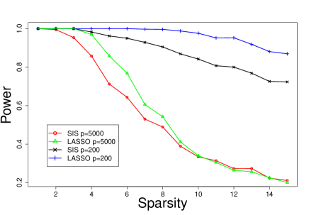
Results. The results are presented on Figure 4. When is
small, the dimension reduction problem is not ultra-high dimensional and the
Lasso and the SIS methods keep all the relevant covariates.
For large , the both methods miss some of the relevant
covariates. For , there is a clear decrease in the power
beyond . For and , both methods only have a power close to
0.5. In expectation, only four covariates belong to the sets
and of size 50. For , there is not a so clear transition,
but the power decreases slowly for . If there was no elbow effect in the minimax risk of estimation, then it would still be possible to recover the support of with high probability. Indeed, each non-zero component of is larger than which is detectable in a reasonable setting (see e.g. [46]). For instance, for and , . Here, the elbow effect implies that even for a huge signal over noise ratio, it is impossible to reduce the dimension of the problem without forgetting relevant variables.
Second simulation setting. We still take , , , , and ranging from 1 to 5. being fixed, we take such that and . Relying on experiments, we estimate the smallest such that has a power larger than . corresponds (up to the renormalization ) to the minimal intensity of the signal so that the dimension reduction method does not forget relevant covariates.

Results. The results are presented on Figure 5. For small , remains close to . In contrast, we observe that blows up at . We have not depicted , but we have . These two simulation studies confirm that when becomes large (in comparison to and ), the dimension reduction problem becomes extremely difficult.
Remark 7.1 (Rule of thumb).
From these simulations and from other theoretical arguments (e.g. [27, 22, 45]), we derive a simple rule of thumb. We say that a problem is ultra-high dimensional if
| . | (7.1) |
For and , this corresponds to . Setting and yields . In practice, we do not know in advance. Nevertheless, this criterion (7.1) helps us to know what is the largest sparsity index such that the statistical problem remains reasonably difficult in the minimax sense.
8 Discussion
As stated in Sections 4–6, the behaviors of the minimax separation distances and of the minimax risks become really different in an ultra-high dimensional setting. Apart from the test problem () with known variance and the problem of prediction () with fixed design, all the other separations distances and minimax risks blow up when becomes larger than .
This elbow effect has important practical implications: there is no hope of
selecting the
relevant covariates in an ultra-high dimensional setting, except if
signal over noise ratio is exponentially large. Moreover, even dimension
reduction techniques cannot work well in such a setting.
In linear testing (), we have proved that the optimal separation
distances highly depend on the knowledge of the variance.
Most of the testing procedures in the
literature rely on the knowledge of
. Some specific work is therefore needed to derive fast
and efficient procedures under unknown variance (but see [34] for a procedure in a specific situation).
We have not discussed so far the problem of variance estimation. From the minimax lower bounds of testing, we deduce the following lower bound.
Proposition 8.1.
Assume that . For any , there exist designs such that
As a consequence, the problem of variance estimation becomes extremely difficult in an ultra-high dimensional setting.
In Propositions 5.3 and
6.1, we have provided minimax lower bounds
for () and () over for arbitrary designs
. Our corresponding upper bounds match these lower bounds when the
restricted eigenvalues of are close to each other. However, these
bounds do not agree anymore when these restricted eigenvalues are away from each other.
Deriving the exact
dependency of the minimax risks on would require sharper lower bounds
and the analysis of
new estimation procedures.
Our minimax results use the Gaussianity of the noise and the Gaussianity of the design in the random design setting. In an ultra-high dimensional setting, the minimax upper bounds do not seem to be robust with respect to the Gaussianity. In smaller dimensions (), the Gaussian distribution of the design is less critical. For instance, consider a design where all the components are independent and follow a subgaussian distribution. By a result of Rudelson and Vershynin [41], the restricted eigenvalues of remain away from with high probability. Consequently, some of the minimax bounds should still hold for subgaussian designs. Nevertheless, the derivation of sharp minimax bounds for non-Gaussian designs and noises remains an open problem
9 Proofs of the minimax lower bounds
Some propositions contain both minimax lower bounds and upper bounds. This section is devoted to the proof of the main lower bounds, while the upper bounds are proved in Appendix B in [43]. In order to keep our notations as short as possible, we set
We also note for the total variation norm. For any subset , , covariance matrix , and any variance , we denote the quantity
the infimum being taken over all tests satisfying . Its counterpart for unknown variance is defined by
the infimum being taken over all tests satisfying . Similarly, we define for fixed design and for fixed design and unknown variance.
Most of the minimax lower bounds in this paper are based on an approach which goes back to Ingster [28, 29, 30]. The following lemma encompasses fixed and random design and known and unknown variance.
Lemma 9.1.
Let be a subset of and let and be two positive integers. Consider a probability measure on . We note and . Then,
| (9.1) | |||||
Here, can be replaced by or . If we also have , then can be replaced by or .
We refer to Baraud [5] Section 7.1 for a proof and further explanations in a close framework. The main idea is to find a prior probability on so that the total variation distance between and is as large as possible. We derive from Lemma 9.1 that if .
9.1 Proof of the lower bound (4.1) in Theorem 4.1
Proof of Theorem 4.1.
By homogeneity, we can assume that . We first build a
suitable prior probability in order to apply Lemma
9.1.
Let us take a set of size uniformly in (defined in Section 2). Let be a sequence of independent Rademacher random variables. Consider some . Define and consider the distribution of the random variable . stands for the distribution of with and . Here, is the orthonormal family of vectors of defined by
The likelihood ratio writes
where stands for the expectation with respect to the distribution of and .
In order to apply Lemma 9.1, we need to upper bound the expectation of . Let us first take the expectation of with respect to .
| (9.2) | |||||
where stands for the expectation with respect to while refers to the expectation with respect to the independent variables , , and .
Lemma 9.2.
If we assume that , then we have
In this lemma, we have specifically distinguished the integration with respect to from the integration with respect to . This will be useful for deriving minimax lower bound in fixed design (Proposition 4.2). Gathering Lemmas 9.1 and 9.2 allows to derive that
This last bound allows to conclude since .
∎
Proof of Lemma 9.2.
Let us fix , , and . First, we shall compute the
expectation
.
Let us decompose the set into four sets (which possibly are empty): , , , and , where and are defined by and . For the sake of simplicity, we reorder the elements of from to such that the first elements belong to , then to and so on.
where is the identity matrix of size and is block symmetric matrix of size defined by
Each block corresponds to one of the four previously defined subsets of (i.e. , , , and ). The matrix is of rank at most four. Hence, has the same determinant as the matrix of size defined by:
After some computations, we lower bound the determinant of
From now on, we assume that so that . Hence, we get
| (9.5) | |||||
Then, we take the expectation with respect to , , and . When and are fixed the expression (9.5) depends on and only through the cardinality of . As and follow independent Rademacher distributions, the random variable follows the distribution of , a sum of independent Rademacher variables and
| (9.6) |
where stands for the expectation with respect to . We now proceed as in the proof of Theorem 1 in Baraud [5] in order to upper bound the term
Following Baraud’s arguments, we get that when
Moreover, we have as soon as since . Gathering these observations with (9.6), we conclude that as soon as
∎
9.2 Proof of the lower bound (4.10) in Theorem 4.3
Proof of (4.10) in Theorem 4.3.
Lemma 9.3.
Suppose that . We have
| (9.7) |
for any such that
| (9.8) |
If we assume that Condition (A.1) holds, (9.7) holds for any such that
| (9.9) |
If and with and large enough, then Assumption is satisfied. For large enough, the quantity is large enough so that the lower bound (9.9) satisfies
Let us now assume that and where has been previously fixed. Then, the first lower bound (9.8) satisfies:
Gathering the two previous lower bounds with Lemma 9.3 allows to conclude. ∎
Proof of Lemma 9.3.
Consider some . To apply Lemma 9.1, we first have to define a suitable prior on and a suitable . More specifically, we set and the distribution is supported by defined by
Let be a random variable uniformly distributed over . Let be the distribution of the random variable where
and where is the orthonormal family of vectors of defined by if and otherwise. By Lemma 9.1, we only have to prove under conditions (9.8) or (9.9) with (), we have
| (9.10) |
Observe here that we use a variance for and a variance for the hypothesis . Using these two different variances allows us to take advantage of the fact that we work under unknown variance.
As a specific case of [44] Eq.(8.5), we have
where follows an hypergeometric distribution with parameters , , and . We know from Aldous (p.173) [2] that follows the same distribution as the random variable where is a binomial random variable of parameters , and some suitable -algebra. By a convexity argument, we get
| (9.11) |
Hence, we only need to upper bound the expectation of the second random variable.
CASE 1: Proof of Equation (9.8). Since and since , we have
As a consequence, the condition (9.10) holds if . Observe that . Since for any and any , the last condition is enforced by .
CASE 2: Proof of Equation (9.9). Here, we bound (9.11) under condition . We have
Since we need to ensure that , it is sufficient to prove that
| (9.12) | |||||
| (9.13) |
In order to prove these bounds, we shall use a deviation inequality of the random variable .
Lemma 9.4.
For any , , it holds that
| (9.14) |
FACT 1.
For any , the upper bounds
(9.12) hold under Condition ().
FACT 2. The upper bound (9.13) holds for any as soon as
| (9.15) |
We derive that under (9.15), we have The fact that allows to conclude.
∎
Proof of FACT 1.
Since for any , we derive that . Gathering this bound with Lemma 9.4, we get a new deviation inequality for .
| (9.16) |
for any . We apply this bound with . Then, Inequality (9.12) holds if
Taking the logarithm of this expression leads to
Since is constrained to be smaller than , we get
By Assumption (A.1), is larger than . Consequently, the worst case among all between and is . Hence, we only need to prove that
Since is larger than , is smaller than and this last inequality is ensured by Assumption (A.1).
∎
Proof of FACT 2.
We consider here the case . We derive from (9.16) that
Consequently, we want to ensure that
for any between and . For any and between and , . Setting and , we obtain that the last inequality holds if
Since is positive, the largest term in the bound corresponds to . Hence, it remains to prove that
We conclude that the upper bounds hold if
∎
Proof of Lemma 9.4.
We prove this deviation inequality using the Laplace transform of . Consider some and .
Deriving with respect to an upper bound of the last expression leads to the following choice
Hence, we get
Since we assume , we conclude that
Since , this upper bound is also valid when . ∎
9.3 Proof of Proposition 5.1
We derive this minimax lower bound from the hypothesis testing problem studied in Section 4. Since the covariance , the loss is simply . For the sake of simplicity, we assume that is even. We split the covariates into two groups and of size . Given some , we fix and we consider the two sets
Take any estimator . We consider an estimator such that
By the triangle inequality, we have , for any .
| (9.17) |
It is enough to prove that for , the supremum of
the probabilities
is lower
bounded by a positive constant.
This is equivalent to lower bounding the minimax separation distance for
against : .
As in the proof of Theorem 4.3, we build a prior distribution on . Consider the collection of subsets of of size . Let be be some random variable uniformly distributed over . Then, is the distribution of . Similarly, we define the prior distribution on . We note . We have
| (9.18) | |||||
by the triangle inequality. Lemma 9.1 states that
where . In fact, the second moment of has been studied in the proof of Theorem 4.3. If we take in this proof, we derive
9.4 Proof of Proposition 5.6
Let us set
.
Consider a design that achieves the bound
(4.13) and take . If is large enough, then .
Take any estimator that does not rely on the variance
. Let us build a test of the
hypotheses
: against
:
:
By Proposition 4.4, we have at least one of the two following properties:
| (9.20) | |||||
| (9.21) |
CASE 1: (9.20) holds. We have for any . Thus, there exists such that with probability larger than . As a consequence, we have
9.5 Proof of Proposition 8.1
For the sake of conciseness, we note . Given a positive number , we note . As in the proof of Theorem 4.3, we consider the prior probability on . For any estimator , we define by . For any , the loss is controlled as follows:
Thus, we get the minimax lower bound
| (9.22) | |||||
Let us note two numbers and . If is a standard Gaussian design and if , then the proof of Theorem 4.3 states for
we have where the expectation is taken both with respect to and . Applying Markov’s inequality, we derive that with positive probability,
For such designs and such we have
since . We conclude that
9.6 Fano’s Lemma
The next lower bounds are established applying Birgé’s version of Fano’s Lemma [10]. More precisely, we shall use the following lemma, which is taken from Corollary 2.19 in [37],
Lemma 9.5.
Let be some pseudo metric space, be some statistical model. Let us note . Then, for any estimator and any finite subset of , setting , provided that the following lower bound holds for any :
9.7 Proof of the lower bounds of Propositions 6.1 and 6.4
This lower bound is based on Fano’s lemma. For the sake of simplicity, we assume that and that . First, we consider a unit vector such that . Let us define . It is possible to find two vectors such that and . Consequently, the Kullback distance between the two distributions and is exactly and . Applying Lemma 9.5, we derive the first part of the lower bound:
Let us turn to the second part of the lower bound. We consider the collections of subsets of of size . Applying combinatorial results such as Varshamov’s lemma and Lemma 4.10 in [37], we derive that there exists of size larger than such that any pairs of distinct sets , in , we have .
For any , we define a vector that satisfies:
-
•
if and else.
-
•
.
Let us prove that this construction is possible by induction on . The construction is straightforward for . Assume that this construction is possible for . Let us take some subset and such that . There exists a vector such that , for any and . Now consider the two vectors and such that if , if and else. It follows that or , which allows to conclude.
For any , we consider the set . The Kullback distance between any two element in is upper bounded as follows:
while we have . Applying Birgé’s version of Fano’s lemma [10] we conclude that:
where stands for the convex hull of . Taking allows to conclude.
9.8 Proof of Proposition 6.2
Proof of the first result. First, the minimax lower bound is a straightforward consequence of (6.2), since if . Let us turn to the upper bound. Thanks to the minimax upper bound (6.1), we only have to prove that there exists a design such that its -restricted eigenvalues remain close from .
Consider a standard Gaussian design of size . Rescaling to a norm of each column of , we get a design . Let us assume that . Applying Lemma 11.2, we control the restricted eigenvalues of :
with probability larger than . Consider any such that . By definition of , there exists some such that . Moreover we have
Hence, we derive that
Thus, we have with positive probability.
Proof of the second result. Let be a design in . Take . Let us consider the collection (defined in Section 2). As explained in the proof of Proposition 6.1, there exists of size larger than such that any pairs of distinct sets , in , we have .
For any , we define a vector such that if and else and that . Such a construction is justified in the proof of Proposition 6.1.
For any in , we have
. If there exist two distinct sets such that , then the design satisfies
. A necessary condition for
to satisfy
is therefore that the vectors are -separated.
If satisfies , then the balls in with radius centered at are all disjoint. Thus, the sum of their volumes, is smaller than the volume of a ball a radius in . This implies that . Hence, for any design with unit columns, we have
which allows to prove the second result.
Proof of the third result. The minimax lower bound is direct consequence of (6.2) and (6.4). In order to finish the proof, we shall combine the minimax upper bound (6.1) with an upper bound of . Consider a standard Gaussian design with size . Applying the deviation inequality (11.3) of Lemma 11.2, we derive that with probability larger than , we have
However, the design does not belong to . This is why we consider , where is a diagonal matrix of size , whose -th diagonal element corresponds to the norm of the -th column of . Obviously, belongs to .
Each diagonal element of follows of distribution with degrees of freedom. Applying Lemma 11.1, we derive that with probability larger than . We conclude that
with probability larger than . This allows to conclude.
9.9 Proof of Proposition 6.6
For the sake of simplicity, we assume that . Consider a design . By the proof of Proposition 6.2, there exist two vectors and such that:
-
1.
and contain exactly non-zero components which are all equal to in absolute value.
-
2.
The Hamming distance between and is larger than .
-
3.
.
Let us set and with . Consequently, the Kullback discrepancy between and is smaller than . Consider an estimator taking its values in . Applying Corollary 2.18 in [37] (which is another version of Fano’s Lemma), we derive that . This allows to conclude.
9.10 Proof of Proposition 6.7
For the sake of simplicity, we assume that and that is even. Consider any estimator of size . We set
| (9.23) |
where the constants , correspond to the ones used at the end of the proof of Proposition 5.1. We also consider the set . Suppose that we have
| (9.24) |
Assume we are given a second -sample of () independent of the first one. We note () this new sample. We consider the estimator defined by
Since , all the covariates that do not lie in the support of play a symmetric role in the distribution of (). This estimator has the same form as the estimator introduced in (10.5). Arguing as in the proof of Theorem 5.2, we derive that
with probability larger than . Gathering this bound with (9.24), we derive that for any , we have
| (9.25) |
with probability larger than .
We shall prove that (9.25) is impossible if is too large. Let us split the covariates into two groups and . We consider the subsets (resp. ) of whose elements have their support in (resp. ). Arguing as in (9.17) and (9.18), we derive that for any estimator , there exists such that
with probability larger than . Here, the constants and are the same as in (9.23).
10 Procedures involved in the proofs of the minimax upper bounds
10.1 Testing procedures
10.1.1 Known variance: test
In order to establish the minimax upper bounds for known variance, we consider the following testing procedure. It is taken from Baraud [5] who applies it in the Gaussian sequence model. In the sequel, denotes the probability for a distribution with degrees of freedom to be larger than . Given a subset of , refers to the orthogonal projection onto the space generated by the vectors .
Definition 10.1.
[Procedure ] Define as the smallest integer such that . For any , we define the statistics by
where is defined in Section 2. We also consider
The procedure is defined by
| (10.1) |
The hypothesis is rejected if is positive.
corresponds to a Bonferroni multiple testing procedure based on a large number of parametric tests of the hypothesis : against : and for any . As a consequence, allows to test the hypothesis : against : . Then, corresponds to a Bonferroni multiple testing procedures based on the statistics , . Obviously, the procedure is computationally intensive. It is used here as a theoretical tool to derive minimax upper bounds.
10.1.2 Unknown variance: test
We introduce a second testing procedure to handle the case of unknown variance .
Definition 10.2.
[Procedure ] Fixing some subset of such that , we note the rank of the subdesign of of size . We define the Fisher statistic by
| (10.2) |
We build the statistic as
| (10.3) |
where denotes the probability for a Fisher variable with and degrees of freedom to be larger than . Finally, the statistic is defined by
| (10.4) |
The hypothesis is rejected when is positive.
In fact, is a Bonferroni multiple testing procedure. Contrary to , it is based on Fisher statistics to handle the unknown variance. The ideas underlying this statistic have been introduced in Baraud et al. [7] in the context of fixed design regression.
10.2 Estimation procedures
10.2.1 Definition of the estimator
Definition 10.3.
[Estimator ] For any integer , we consider a least-squares estimator defined by
| (10.5) |
Let us define the penalty function by
| (10.6) |
where is a tuning parameter. The dimension is selected as follows
For short, we note .
This variable selection procedure relies on complexity penalization. The penalty depends on the size of and on the number of subsets of of size . Observe that the estimator does not require the knowledge of .
10.2.2 Definition of the estimator and proof of (5.6) in Proposition 5.3
Definition 10.4.
[Procedure for fixed design regression] Define as the smallest integer such that . Let us consider the collection of dimensions . Then, the penalty function is defined by
We recall that for , the estimators are defined in (10.5) and that . The size is selected by minimizing the following penalized criterion
| (10.8) |
For short, we write .
11 Deviation inequalities
The proofs of the deviation inequalities stated in this section are postponed to Appendix C in [43].
Lemma 11.1 ( distributions).
For any integer and any number ,
For any positive number
| (11.1) |
where the constant .
Lemma 11.2 (Wishart distributions).
Let be a standard Wishart matrix of parameters with . For any number ,
| (11.2) |
For any with and any number ,
| (11.3) |
where is a numerical constant.
The two first deviation inequalities are taken from Theorem 2.13 in [19]. The bound (11.3) allows to control the tail distribution of the smallest eigenvalue of a Wishart distribution. Rudelson and Vershynin [41] have provided a control similar to (11.3) under subgaussian assumptions. However, their results only holds for events of probability smaller than .
Acknowledgements
I am grateful to Yannick Baraud and Christophe Giraud, the Associate Editor, and two anonymous referees for suggestions that greatly improve the presentation of the paper.
References
- [1] Abramovich, F. and Grinshtein, V. (2010). MAP model selection in Gaussian regression. Electron. J. Stat. 4, 932–949. http://dx.doi.org/10.1214/10-EJS573. \MR2721039 (2011j:62028)
- [2] Aldous, D. J. (1985). Exchangeability and related topics, École d’été de probabilités de Saint Flour XIII. Lecture Notes in Mathematics, Vol. 1117. Springer-Verlag, Berlin.
- [3] Arias-Castro, E., Candès, E. J., and Plan, Y. (2010). Global testing and sparse alternatives: Anova, multiple comparisons and the higher criticism. arXiv:1007.1434.
- [4] Baraniuk, R., Davenport, M., DeVore, R., and Wakin, M. (2008). A simple proof of the restricted isometry property for random matrices. Constr. Approx. 28, 3, 253–263. http://dx.doi.org/10.1007/s00365-007-9003-x. \MRMR2453366
- [5] Baraud, Y. (2002). Non-asymptotic rates of testing in signal detection. Bernoulli 8, 5, 577–606.
- [6] Baraud, Y., Giraud, C., and Huet, S. (2009). Gaussian model selection with an unknown variance. Ann. Statist. 37, 2, 630–672.
- [7] Baraud, Y., Huet, S., and Laurent, B. (2003). Adaptive tests of linear hypotheses by model selection. Ann. Statist. 31, 1, 225–251. \MRMR1962505 (2004a:62091)
- [8] Bickel, P., Ritov, Y., and Tsybakov, A. (2009). Simultaneous analysis of lasso and Dantzig selector. Ann. Statist. 37, 4, 1705–1732. http://dx.doi.org/10.1214/08-AOS620. \MRMR2533469
- [9] Birgé, L. (2001). An alternative point of view on Lepski’s method. In State of the art in probability and statistics (Leiden, 1999). IMS Lecture Notes Monogr. Ser., Vol. 36. Inst. Math. Statist., Beachwood, OH, 113–133. http://dx.doi.org/10.1214/lnms/1215090065. \MRMR1836557 (2002j:62049)
- [10] Birgé, L. (2005). A new lower bound for multiple hypothesis testing. IEEE Trans. Inform. Theory 51, 4, 1611–1615. \MRMR2241522 (2007b:62024)
- [11] Birgé, L. and Massart, P. (2001). Gaussian model selection. J. Eur. Math. Soc. (JEMS) 3, 3, 203–268. \MRMR1848946 (2002i:62072)
- [12] Birgé, L. and Massart, P. (2007). Minimal penalties for Gaussian model selection. Probab. Theory Related Fields 138, 1-2, 33–73. http://dx.doi.org/10.1007/s00440-006-0011-8. \MRMR2288064 (2008g:62070)
- [13] Candès, E. and Plan, Y. (2009). Near-ideal model selection by minimization. Ann. Statist. 37, 5A, 2145–2177. http://dx.doi.org/10.1214/08-AOS653. \MRMR2543688
- [14] Candes, E. J. and Tao, T. (2005). Decoding by linear programming. IEEE Trans. Inform. Theory 51, 12, 4203–4215. http://dx.doi.org/10.1109/TIT.2005.858979. \MRMR2243152 (2007b:94313)
- [15] Candes, E. J. and Tao, T. (2007). The Dantzig selector: statistical estimation when is much larger than . Ann. Statist. 35, 6, 2313–2351. \MRMR2382644
- [16] Chu, J.-H., Weiss, S., Carey, V., and Rabyl, B. (2009). A graphical model approach for inferring large-scale networks integrating gene expression and genetic polymorphism. BMC Systems Biology 3:55.
- [17] Cook, R. D. and Li, B. (2002). Dimension reduction for conditional mean in regression. Ann. Statist. 30, 2, 455–474. http://dx.doi.org/10.1214/aos/1021379861. \MRMR1902895 (2003c:62087)
- [18] Dalalyan, A. and Tsybakov, A. (2008). Aggregation by exponential weighting, sharp oracle inequalities and sparsity. Machine Learning 72, 1-2, 39– 61.
- [19] Davidson, K. R. and Szarek, S. J. (2001). Local operator theory, random matrices and Banach spaces. In Handbook of the geometry of Banach spaces, Vol. I. North-Holland, Amsterdam, 317–366. \MRMR1863696 (2004f:47002a)
- [20] Donoho, D. and Jin, J. (2004). Higher criticism for detecting sparse heterogeneous mixtures. Ann. Statist. 32, 3, 962–994. http://dx.doi.org/10.1214/009053604000000265. \MRMR2065195 (2005e:62066)
- [21] Donoho, D. and Johnstone, I. (1994). Minimax risk over -balls for -error. Probab. Theory Related Fields 99, 2, 277–303. http://dx.doi.org/10.1007/BF01199026. \MRMR1278886 (95g:62019)
- [22] Donoho, D. and Tanner, J. (2009). Observed universality of phase transitions in high-dimensional geometry, with implications for modern data analysis and signal processing. Philos. Trans. R. Soc. Lond. Ser. A Math. Phys. Eng. Sci. 367, 1906, 4273–4293. With electronic supplementary materials available online, http://dx.doi.org/10.1098/rsta.2009.0152. \MR2546388 (2010k:62407)
- [23] Donoho, D. L. (2006). Compressed sensing. IEEE Trans. Inform. Theory 52, 4, 1289–1306. http://dx.doi.org/10.1109/TIT.2006.871582. \MR2241189 (2007e:94013)
- [24] Efron, B., Hastie, T., Johnstone, I., and Tibshirani, R. (2004). Least angle regression. Ann. Statist. 32, 2, 407–499. With discussion, and a rejoinder by the authors. \MRMR2060166 (2005d:62116)
- [25] Fan, J. and Lv, J. (2008). Sure independence screening for ultrahigh dimensional feature space. J. R. Statist. Soc. B 70, 5, 849–911.
- [26] Fukumizu, K., Bach, F., and Jordan, M. I. (2009). Kernel dimension reduction in regression. Ann. Statist. 37, 4, 1871–1905. http://dx.doi.org/10.1214/08-AOS637. \MRMR2533474
- [27] Giraud, C. (2008). Estimation of Gaussian graphs by model selection. Electron. J. Stat. 2, 542–563.
- [28] Ingster, Y. (1993a). Asymptotically minimax hypothesis testing for nonparametric alternatives I. Math. Methods Statist. 2, 85–114.
- [29] Ingster, Y. (1993b). Asymptotically minimax hypothesis testing for nonparametric alternatives II. Math. Methods Statist. 3, 171–189.
- [30] Ingster, Y. (1993c). Asymptotically minimax hypothesis testing for nonparametric alternatives III. Math. Methods Statist. 4, 249–268.
- [31] Ingster, Y. (1998). Minimax detection of a signal for -balls. Math. Methods Statist. 7, 4, 401–428 (1999). \MR1680087 (2000f:62012)
- [32] Ingster, Y. (2001). Adaptive detection of a signal of growing dimension I. Math. Methods Statist. 10, 4, 395–421.
- [33] Ingster, Y. (2002). Adaptive detection of a signal of growing dimension II. Math. Methods Statist. 11, 1, 37–68.
- [34] Ingster, Y., Tsybakov, A., and Verzelen, N. (2010). Detection boundary in sparse regression. Electron. J. Stat. 4, 1476–1526.
- [35] Johnstone, I. (1994). On minimax estimation of a sparse normal mean vector. Ann. Statist. 22, 1, 271–289. http://dx.doi.org/10.1214/aos/1176325368. \MRMR1272083 (95g:62020)
- [36] Lounici, K. (2008). Sup-norm convergence rate and sign concentration property of Lasso and Dantzig estimators. Electron. J. Stat. 2, 90–102. http://dx.doi.org/10.1214/08-EJS177. \MRMR2386087 (2009a:62287)
- [37] Massart, P. (2007). Concentration inequalities and model selection. Lecture Notes in Mathematics, Vol. 1896. Springer, Berlin. Lectures from the 33rd Summer School on Probability Theory held in Saint-Flour, July 6–23, 2003, With a foreword by Jean Picard. \MRMR2319879 (2010a:62008)
- [38] Meinshausen, N. and Bühlmann, P. (2006). High-dimensional graphs and variable selection with the lasso. Ann. Statist. 34, 3, 1436–1462. \MRMR2278363 (2008b:62044)
- [39] Raskutti, G., Wainwright, M., and Yu, B. (2009). Minimax rates of estimations for high-dimensional regression over balls. Tech. rep., UC Berkeley.
- [40] Rigollet, P. and Tsybakov, A. (2011). Exponential screening and optimal rates of sparse estimation. Ann. Statist. 39, 2, 731–771.
- [41] Rudelson, M. and Vershynin, R. (2009). Smallest singular value of a random rectangular matrix. Comm. Pure Appl. Math. 62, 12, 1707–1739. http://dx.doi.org/10.1002/cpa.20294. \MRMR2569075
- [42] Verzelen, N. (2010a). High-dimensional gaussian model selection on a gaussian design. Ann. Inst. H. Poincaré Probab. Statist. 46, 2, 480–524.
- [43] Verzelen, N. (2010b). Technical Appendix to ”Minimax risks for sparse regressions: Ultra-high-dimensional phenomenons.”. http://nicolas.verzelen.free.fr/pdf/2012-Ver-Ultra-appendix.pdf.
- [44] Verzelen, N. and Villers, F. (2010). Goodness-of-fit tests for high-dimensional Gaussian linear models. Ann. Statist. 38, 2, 704–752. \MRMR2604699
- [45] Wainwright, M. (2009a). Information-theoretic limits on sparsity recovery in the high-dimensional and noisy setting. IEEE Trans. Inform. Theory 55, 12, 5728–5741. http://dx.doi.org/10.1109/TIT.2009.2032816. \MRMR2597190
- [46] Wainwright, M. (2009b). Sharp thresholds for high-dimensional and noisy sparsity recovery using -constrained quadratic programming (lasso). IEEE Trans. Inform. Theory 55, 5, 2183–2202.
- [47] Ye, F. and Zhang, C.-H. (2010). Rate minimaxity of the Lasso and Dantzig selector for the loss in balls. J. Mach. Learn. Res. 11, 3519–3540. \MR2756192
- [48] Yu, B. (1997). Assouad, Fano, and Le Cam. In Festschrift for Lucien Le Cam. Springer, New York, 423–435. \MRMR1462963 (99c:62137)
- [49] Zhao, P. and Yu, B. (2006). On model selection consistency of Lasso. J. Mach. Learn. Res. 7, 2541–2563. \MRMR2274449
- [50] Zou, H. and Hastie, T. (2005). Regularization and variable selection via the elastic net. J. R. Stat. Soc. Ser. B Stat. Methodol. 67, 2, 301–320. \MRMR2137327