Derivation of the $t$-$J$ model for finite doping

Abstract

Mapping complex problems to simpler effective models is a key tool in theoretical physics. One important example in the realm of strongly correlated fermionic systems is the mapping of the Hubbard model to a $t$-$J$ model which is appropriate for the treatment of doped Mott insulators. Charge fluctuations across the charge gap are eliminated. So far the derivation of the $t$-$J$ model is only known at half-filling or in its immediate vicinity. Here we present the necessary conceptual advancement to treat finite doping. The results for the ensuing coupling constants are presented. Technically, the extended derivation relies on self-similar continuous unitary transformations (sCUT) and normal-ordering relative to a doped reference ensemble. The range of applicability of the derivation of $t$-$J$ model is determined as function of the doping $\delta$ and the ratio bandwidth $W$ over interaction $U$.

I Introduction

The Hubbard model Gutzwiller (1963); Hubbard (1963); Kanamori (1963) is one of the most common models for the description of strongly correlated electron systems on lattices. Because it contains the motion of the electrons as well as the interaction between two electrons at the same site it is capable to describe charge degrees of freedom as well as magnetic degrees of freedom. Due to the rich physical behavior of the Hubbard model an analytic solution is not possible except in one dimension Essler et al. (2005).

One common route to simplify the model for large repulsion $U$ is to derive an effective model which does no longer contain charge fluctuations across the charge gap. Processes which change the number of doubly occupied sites (double occupancies, DOs) are eliminated. For large enough repulsion $U$ and at half-filling the electrons are fixed on their lattice sites. In this Mott-insulating phase the model can be mapped onto a Heisenberg model describing only the energetically low-lying spin degrees of freedom. In the immediate vicinity of half-filling the motion and the interaction of doped holes is described by the extension of the Heisenberg model to the $t$-$J$ model Harris and Lange (1967); Takahashi (1977); MacDonald et al. (1988); Stein (1997); Reischl et al. (2004). The metallic behavior for small values of the repulsion is beyond the applicability of this mapping Millis and Coppersmith (1991).

In the present work the mapping of the Hubbard model to the $t$-$J$ model is extended to finite macroscopic doping concentration $\delta$. The influence of the doping $\delta$ on the resulting parameters of the $t$-$J$ model is studied for sufficiently large repulsion. Our approach provides a systematic and controlled derivation of the effective coupling constants as function of the doping concentration. Thereby, an important gap between the applicability of the derivation of the $t$-$J$ model and its actual applications is closed.

First, we consider the half-filled case. The elimination of the charge fluctuations across the charge gap is performed by a self-similar continuous unitary transformation with various types of generators. Besides the magnetic exchange couplings, the resulting $t$-$J$ model contains the motion and the interaction of holes and doubly occupied sites. Since the mapping starts from a reference ensemble comprising the two spin states with equal weight and without any correlations between the spins on neighboring sites the spin state in the effective model remains unspecified.

The mapping relies on the elimination of processes changing the number of holes and doubly occupied sites. Note that an empty site represents a double occupancy of two holes. In the half-filled case the density of states exhibits two distinct bands for large $U$ (see Fig.  1). The bands display equal weight $1/2$ and they are well separated for large $U$ Hubbard (1963, 1964a, 1964b); Georges et al. (1996). Thus the states without holes or doubly occupied sites are energetically well separated from the ones with one or more holes or doubly occupied sites. If $U$ is decreased the bands approach each other. As soon as they touch the insulating phase is no longer the appropriate phase and metallic behavior occurs resulting in the breakdown of the mapping to the $t$-$J$ model.

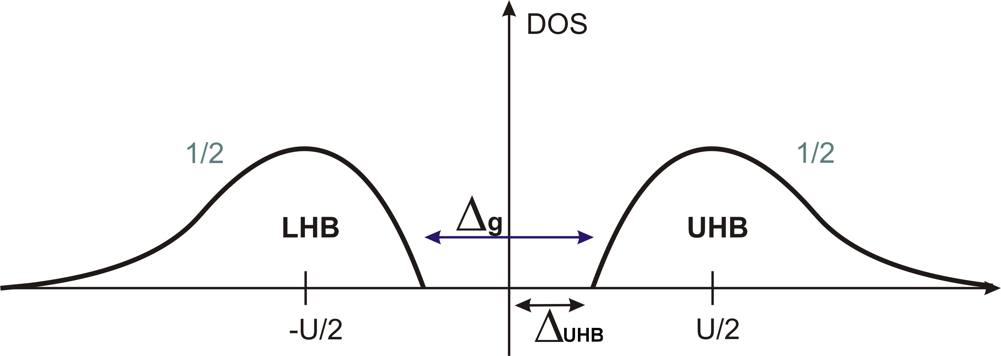
Figure 1: (Color online) Density of states for the half-filled Hubbard model with large repulsion $U$ Gutzwiller (1963); Hubbard (1963); Kanamori (1963). The density of states exhibits two distinct, equally weighted bands, the lower Hubbard band (LHB) and the upper Hubbard band (UHB) Hubbard (1963, 1964a, 1964b); Georges et al. (1996).

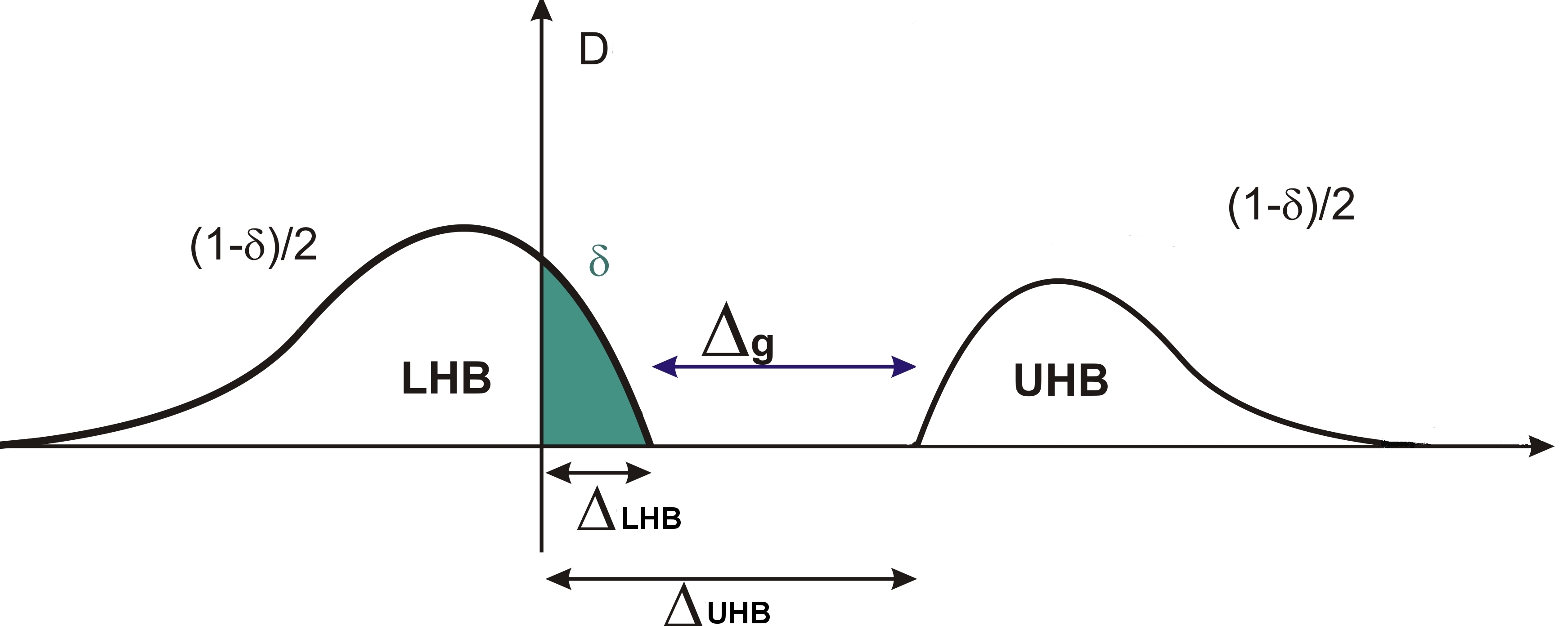
Figure 2: (Color online) Density of states for the case of hole doping with a doping concentration $\delta$. The weight of the hole state is given by $\delta$. The two half-filled states both carry the weight $\frac{1-\delta}{2}$. Note that the weight of the lower band is larger than the one of the upper Hubbard band Jarrell et al. (1995).

The generic density of states obtained in the doped case is depicted in Fig. 2. The effect of the doping on the density of states consists in shifting the Fermi energy into the lower Hubbard band for hole doping and redistributing the weight of the bands. Electron doping is completely analogous in shifting the Fermi energy into the upper Hubbard band. Since we focus here on particle-hole symmetric, bipartite lattices we will consider hole doping without loss of generality.

It is obvious from the comparison of Fig.  1 with Fig. 2 that the energetic separation of the Hubbard bands is more subtle in the doped case than in the half-filled case. The bands are shifted depending on $\delta$ and spectral weight is transferred as well. The shift of spectral weight is a smoking gun evidence for strongly correlated fermionic systems.

Simple counting arguments in the limit $U\rightarrow\infty$ tell us the distribution of weight. Adding an $\uparrow$ electron to a site succeeds with probability $p=\delta+(1-\delta)/2$. The first term results from the fraction of empty sites; the corresponding weight is found at low energy because no doubly occupied site has to be created. The second term results from the fraction of sites occupied by $\downarrow$ electrons; the corresponding weight is found at about $\omega\approx U$ because a doubly occupied site is created. Together with the sum rule the weights shown in Fig. 2 result.

We continue to use the number of doubly occupied sites (DOs) as criterion to distinguish different sectors of the Hilbert space. In order to have a quantitative measure for the energy separation of the sectors with differing number of DOs the apparent charge gap $\Delta_{g}$ is introduced which measures the energy separation of subspaces. It does not measure the energy gap between two pure states which is the reason why we call this separation of energy scales “apparent”. While the apparent charge gap is not an energy gap in a rigorous sense it is experimentally significant: It quantifies the energy needed in an Mott insulator to create a charge excitation irrespective of the spin state of the system. For instance, the system can be at a temperature which implies a disordered paramagnetic spin state while it preserves the insulating properties.

In the half-filled case the apparent charge gap measures the minimal energy of a doubly occupied site moving in an arbitrary spin background. The apparent charge gap is reduced for increasing values of the band width $W$. If the gap vanishes the system is no longer stable against charge fluctuations and the mapping fails Millis and Coppersmith (1991).

Obviously, the physical properties of strongly interacting fermionic systems depend considerably on the doping level Damascelli et al. (2003). This fact leads automatically to the question how the validity of the mapping from the Hubbard model to a generalized $t$-$J$ model is influenced by doping. Thus the apparent charge gap has to be determined in dependence on the doping $\delta$. Keeping track of the apparent charge gap we determine the parameter range in which the mapping is still justified. This range of applicability may not be misinterpreted as phase diagram although it has some similarities Millis and Coppersmith (1991). For instance, for large repulsion $U$ a doped $t$-$J$ model is still perfectly well defined while it displays metallic behavior. Of course, it is expected that the applicability of a $t$-$J$ model decreases upon increasing doping Millis and Coppersmith (1991).

In view of the above, it is one of our central objectives to derive a diagram showing the range of applicability in dependence on the doping which has, to our knowledge, not been done before. Our findings provide access to the limitations of the use of $t$-$J$ models in the context of planar cuprates to the extent that they can be described by a single-band Hubbard model.

The approach used is based on two conceptual ingredients. The first is a systematically controlled change of basis by means of continuous unitary transformations Wegner (1994); Stein (1997); Reischl et al. (2004). The second is the choice of a doped reference ensemble without spin or charge order. Within the range of applicability the effective $t$-$J$ model is derived. The doping dependence of the effective coupling constants is studied. The results are given in dependence on the ratio $W/U$ and on the dopant concentration $\delta$. The method implemented here uses a self-similar truncation scheme to reduce the amount of proliferating terms in the running Hamiltonian. The truncation is performed according to the range of the processes, that means rather local processes are kept while ones of longer range are neglected. Hence the local processes acquire a non-perturbative dependence on the bare, initial coupling constants of the system.

Furthermore, recently introduced modified generators of the CUT are implemented to cope with the vast amount of terms arising during the transformation Fischer et al. (2010). Their results are very close to the previously used particle-conserving generator Mielke (1998); Knetter and Uhrig (2000); Reischl et al. (2004), but they significantly facilitate the calculation in terms of required memory and CPU time.

After this introduction, the model and the method (see Sects. II, III) are introduced. In Sect. VI results for the apparent charge gap are presented and Sect. VII provides exemplary results for the doping dependence of the coupling constants. Sect. VIII concludes the article.

II Hubbard Model

We consider the fermionic Hubbard model Hubbard (1963); Kanamori (1963); Gutzwiller (1963). It describes electrons with spin $\sigma$ on a lattice site $i$ by their creation operator $\hat{c}_{i,\sigma}^{\dagger}$ and their annihilation operator $\hat{c}_{i,\sigma}^{\phantom{\dagger}}$. The Hamiltonian consists of two terms describing the single-fermion kinetics ($H_{t}$) and their interaction ($H_{U}$)

$$H =H_{t}+H_{U}$$ (1a)

$$H_{t} =t\sum_{<i,j>}(\hat{c}_{i\sigma}^{\dagger}\hat{c}_{j\sigma}^{\phantom{\dagger}}+\text{h.c.})$$ (1b)

$$H_{U} =U\sum_{i}\left(\hat{n}_{i,\uparrow}-\frac{1}{2}\right)\left(\hat{n}_{i,\downarrow}-\frac{1}{2}\right).$$ (1c)

The kinetic part consists of the hopping of an electron with spin $\sigma$ from site $i$ to site $j$ and vice versa. For this process to take place $i$ and $j$ have to be nearest neighbors as indicated by the bracket under the sum. The corresponding matrix element is denoted by $t$. The band width $W$ of the model is given by $W=2zt$ with the coordination number $z$ (number of nearest neighbors). In this work the lattice studied is the two dimensional square lattice with coordination number $z=4$ so that $W=8t$.

The second part of the Hamiltonian determines the interaction of the electrons. This term constitutes a pure on-site interaction. In $H_{U}$ the operator $\hat{n}_{i,\sigma}=\hat{c}_{i,\sigma}^{\dagger}\hat{c}_{i,\sigma}^{\phantom{\dagger}}$ represents the number operator for the electrons. This indicates that putting two electrons on the same site costs the additional energy $U$.

In the Hubbard model there are four possible states per site. The site may be singly occupied by one electron with spin up or spin down $|\uparrow\rangle$,$|\downarrow\rangle$, doubly occupied by two electrons with opposite spin $|\downarrow\uparrow\rangle$ or completely empty $|0\rangle$. The last two configurations correspond to charge fluctuations and are referred to as double occupancies (DO) in this context.

The interplay of motion and interaction of electrons in the Hubbard model provides a description of the metal-insulator transition Imada et al. (1998). Another important field of application of the single-band Hubbard model is the physics of high-$T_{\text{C}}$ cuprates Bednorz and Müller (1986); Lee et al. (2006).

For a large Hubbard repulsion $U$ in the half-filled case the density of states exhibits two separate bands, see Fig. 1, the so-called lower (LHB) and the upper Hubbard band (UHB). For infinite $U$ each site of the lattice is occupied by one electron which is energetically fixed to its site. If $U$ is finite the electron can move and virtually hop to adjacent site. Thereby, DOs are created but the the physics remains rather local, that means, the charge correlation length stays small.

Based on the locality of the important processes one may map the Hubbard model onto an effective $t$-$J$ model. The generalized $t$-$J$ model conserves the number of DOs. It comprises a part which describes the magnetic degrees of freedom, which is a generalized Heisenberg model, and a part which describes the motion and interaction of DOs reflecting the charge degrees of freedom. In order to obtain a model conserving the number of DOs, processes which create or annihilate DOs have to be eliminated. One systematic way to achieve this objective is the application of continuous unitary transformations to the Hamiltonian.

For smaller values of $U$ the local picture used here is no longer appropriate and the derivation of the $t$-$J$ model is not justified.

III Continuous Unitary Transformations

III.1 General Framework

The effective $t$-$J$ model is derived from the Hubbard model by eliminating processes which change the number of DOs. This elimination is performed using continuous unitary transformations (CUT) Wegner (1994); Stein (1997); Mielke (1998); Knetter and Uhrig (2000); Reischl et al. (2004); Fischer et al. (2010). The elimination is based on a systematic change of the basis

$$H(\ell)=\hat{U}^{\phantom{\dagger}}(\ell)H^{\phantom{\dagger}}\hat{U}^{\dagger}(\ell)$$ (2)

with a unitary operator $\hat{U}$ and a continuous auxiliary variable $\ell$ referred to as the flow parameter. The transformation is determined by the flow equation

$$\frac{d}{d\ell}H(\ell)=\left[\eta(\ell),H(\ell)\right]$$ (3)

where $\eta(\ell)$ denotes an antihermitian infinitesimal generator. At $\ell=0$ the transformation starts with the initial Hamiltonian $H$. The unitary transformation can be stopped at any arbitrary value of the flow parameter $\ell$. Usually, the effective Hamiltonian is reached for $\ell=\infty$. Due to the continuity of the transformation it is readjusted to the flowing Hamiltonian for every value of $\ell$.

The transformation stops automatically when the commutator $[H(\ell),\eta(\ell)]$ vanishes which is generically the case for $\ell\rightarrow\infty$, i.e., for convergence for $\ell\rightarrow\infty$. The structure of the effective Hamiltonian is determined by the choice of the generator $\eta(\ell)$. We first choose the generator which leads to an effective model conserving the number of DOs. To this end, we introduce the operator

$$\hat{D}:=\sum_{i}[\hat{n}_{i,\uparrow}\hat{n}_{i,\downarrow}+\left(1-\hat{n}_{i,\uparrow}\right)\left(1-\hat{n}_{i,\downarrow}\right)]$$ (4)

counting the number of DOs.

By the use of $\hat{D}$ the repulsive part of the Hamiltonian can be written as

$$\hat{H}_{U}=\frac{U}{2}\left(\hat{D}-\frac{N}{2}\right)$$ (5)

with $N$ denoting the number of sites. The kinetic part is split into three parts according to their effect on the number of DOs

$$\hat{H}_{t} =\hat{T}_{0}+\hat{T}_{+2}+\hat{T}_{-2}$$ (6)

where $\hat{T}_{i}$ creates $i$ DOs. The terms are given by

$$\hat{T}_{0}=t_{0}\sum_{<i,j>,\sigma}\left[\left(1-\hat{n}_{i,\sigma}\right)\hat{c}_{i,\bar{\sigma}}^{\dagger}\hat{c}_{j,\bar{\sigma}}^{\phantom{\dagger}}\left(1-\hat{n}_{j,\sigma}\right)+\right.$$

$$\left.\hat{n}_{i,\sigma}\hat{c}_{i,\bar{\sigma}}^{\dagger}\hat{c}_{j,\bar{\sigma}}^{\phantom{\dagger}}\hat{n}_{j,\sigma}+\text{h.c.}\right]$$ (7a)

$$\hat{T}_{+2}=t_{+2}\sum_{<i,j>,\sigma}\left[\hat{n}_{i,\sigma}\hat{c}_{i,\bar{\sigma}}^{\dagger}\hat{c}_{j,\bar{\sigma}}^{\phantom{\dagger}}\left(1-\hat{n}_{j,\sigma}\right)+\right.$$

$$\left.\hat{n}_{j,\sigma}\hat{c}_{j,\bar{\sigma}}^{\dagger}\hat{c}_{i,\bar{\sigma}}^{\phantom{\dagger}}\left(1-\hat{n}_{i,\sigma}\right)\right]$$ (7b)

$$\hat{T}_{-2}=t_{-2}\sum_{<i,j>,\sigma}\left[\left(1-\hat{n}_{i,\sigma}\right)\hat{c}_{i,\bar{\sigma}}^{\dagger}\hat{c}_{j,\bar{\sigma}}^{\phantom{\dagger}}\hat{n}_{j,\sigma}+\right.$$

$$\left.\left(1-\hat{n}_{j,\sigma}\right)\hat{c}_{j,\bar{\sigma}}^{\dagger}\hat{c}_{i,\bar{\sigma}}^{\phantom{\dagger}}\hat{n}_{i,\sigma}\right]\,.$$ (7c)

with $\bar{\sigma}:=-\sigma$.

The terms contained in $T_{0}$ have no effect on the number of DOs while the terms in $T_{+2}$($T_{-2}$) increase (decrease) the number of DOs by two. These terms are the ones that we intend to eliminate by the transformation. In the initial Hamiltonian the prefactors $t_{+2}$,$t_{-2}$ and $t_{0}$ are equal, but they evolve differently under the CUT.

The first generator we use, the so-called quasiparticle conserving generator $\eta_{\text{pc}}$, can be expressed by the commutator

$$\eta_{\text{pc}}(\ell)=\left[\hat{D},\hat{H}(\ell)\right]\,.$$ (8)

This generator corresponds to the generator defined in Refs. Mielke, 1998; Knetter and Uhrig, 2000; Reischl et al., 2004; Fischer et al., 2010 except for a global factor of two, which just implies a multiplicative renormalization of the flow parameter. The terms comprised by this generator are sketched in Fig. 3. The terms of the Hamiltonian are classified according to their number of quasiparticle creation and annihilation operators. The $\left(j,l\right)$ block consists of terms with $j$ creation and $l$ annihilation operators. Note that such a term requires at least $l$ excitations to be present in order to become active. But it is also active if more than $l$ excitations are present in the system. In this respect, the scheme in Fig. 3 may not be mistaken to be a matrix. For a comprehensive presentation we refer the reader to Ref. Fischer et al., 2010.

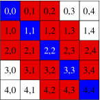
Figure 3: (Color online) Schematic diagram of the Hamiltonian with the terms contained in the $\eta_{\text{pc}}$ generator highlighted in red (dark grey). These terms will be eliminated. The terms in the uncoloured squares are zero initially and stay zero in the flow induced by $\eta_{\text{pc}}$.

The quasiparticle conserving generator $\eta_{\text{pc}}$ comprises all terms of the off-diagonal blocks. Due to the structure of the generator the block-band structure of the Hamiltonian is preserved during the flow Mielke (1998); Knetter and Uhrig (2000); Dusuel and Uhrig (2004). During the whole flow there will only be terms created which change the number of DOs by $0,+2$ or $-2$.

With the definition (8) of the generator the flow equation (3) can be calculated. Comparing the contributions on both sides of Eq. 3 a set of differential equations for the prefactors of the monomials in the creation and annihilation operators is obtained. These differential equations are first order in $\ell$ and they are bilinear in the prefactors entering on the right hand side.

The equations do not form a closed set because in infinite systems new terms continue to arise on each application of the commutator in (3). For $\ell=0$ these terms carry the prefactor zero because they are not part of the initial Hamiltonian. If we kept all these new terms in the remaining calculations we would obtain exact results for the effective model. But the number of arising terms is rising exponentially so that we have to limit them in number. For this purpose a truncation scheme is introduced which specifies the relevance of all term. Less important terms are neglected, leading to a closed set of differential equations which can be solved numerically.

In many previous applications a small parameter is used to classify the arising terms so that a perturbative treatment results. In contrast, we are adopting here a truncation scheme which classifies the terms according to their structure. Such a CUT scheme is usually called self-similar. It resembles more conventional renormalizations. Effects of infinite order are present in the prefactors of the kept terms.

The truncation scheme used in this work keeps or neglects terms according to their locality, i.e., according to the range of the represented physical process. This approach is well justified if the model under study is governed by a small correlation length. This is exactly the case for a Hubbard model at large $U$ where the propagation of charge degrees of freedom is suppressed by the high energetic cost of creating a DO.

III.2 Reference Ensemble and Normal Order

Before we discuss how we measure the degree of locality we have to find a unique representation for the operators to be sure to treat similar terms in the same way. To this end, the monomials are expressed as normal-ordered products of local operators. The normal-ordering we are using is not the standard one known for the fermionic or bosonic algebra because the creation or annihilation of a DO can not be represented by interaction free fermions or bosons. Instead, we use a reference ensemble. Non-trivial operators are only those which create or annihilate fluctuations away from the reference ensemble. For a given doping concentration $\delta$ the reference ensemble is defined by the statistical operator

$$\hat{\rho}_{\delta}=\Pi_{i}\left\{\frac{1-\delta}{2}\Big{[}|\uparrow\rangle_{i}\langle\uparrow|_{i}+|\downarrow\rangle_{i}\langle\downarrow|_{i}\Big{]}+\delta|0\rangle_{i}\langle 0|_{i}\right\}$$ (9)

where the product extends over all lattice sites $i$. In the half-filled case ($\delta=0$) the reference ensemble is paramagnetic and the magnetic degrees of freedom are totally disordered. Each site is equally probably occupied by an $\uparrow$ or by a $\downarrow$ electron; no direction is singled out, no correlation between neighboring sites exists. Charge fluctuations from this reference ensemble are the empty $|0\rangle$ and the doubly occupied site $|\downarrow\uparrow\rangle$. Magnetic fluctuations are induced by the application by spin operators, see below.

Considering doping we focus on hole doping only because the model at hand is particle-hole symmetric so that electron doping leads exactly to the same results. Hence we include the empty state $|0\rangle$ in the reference ensemble (9) besides the half-filled states with a probability given by the doping level $\delta$. The remaining weight is again equally distributed over the two spin states. Note that this extension to the doped case does not introduce any bias. There is no correlation between sites nor on each site. Hence the reference ensemble (9) is the mixture with the maximum entropy at given level of doping.

Based on the reference ensemble we define a term as normal-ordered if the expectation value of each of its factors of local operators vanishes with respect to this ensemble. Thus a normal-ordered local operator fulfills

$$\langle A_{i}\rangle_{\text{ref}} =\delta\langle 0|_{i}A_{i}|0\rangle_{i}+\frac{1-\delta}{2}\left(\langle\uparrow|_{i}A_{i}|\uparrow\rangle_{i}+\langle\downarrow|_{i}A_{i}|\downarrow\rangle_{i}\right)$$

$$=0.$$ (10)

Based on this condition we define a basis of local normal-ordered operators (see Tab. 1). Of course, the identity does not fulfull the condition (10). But the identity is the trivial action of an operator and obviously does not create or annihilate any fluctuation away from the reference ensemble. Without the identity the list of operators would not be complete. Any monomial occuring during the flow is expressed in the operator basis in Tab. 1.

bosonic	fermionic
$\mathds{1}$	$\left(1-\hat{n}_{\downarrow}\right)\hat{c}_{\uparrow}^{\phantom{\dagger}}$
$\sigma^{z}=\hat{n}_{\uparrow}-\hat{n}_{\downarrow}$	$\left(1-\hat{n}_{\uparrow}\right)\hat{c}_{\downarrow}^{\phantom{\dagger}}$
$\hat{c}_{\uparrow}^{\dagger}\hat{c}_{\downarrow}^{\phantom{\dagger}}$	$\hat{n}_{\downarrow}\hat{c}_{\uparrow}$
$\hat{c}_{\downarrow}^{\dagger}\hat{c}_{\uparrow}^{\phantom{\dagger}}$	$\hat{n}_{\uparrow}\hat{c}_{\downarrow}$
$\hat{c}_{\downarrow}\hat{c}_{\uparrow}$	$\hat{n}_{\uparrow}\hat{c}_{\downarrow}^{\dagger}$
$\hat{c}_{\uparrow}^{\dagger}\hat{c}_{\downarrow}^{\dagger}$	$\hat{n}_{\downarrow}\hat{c}_{\uparrow}^{\dagger}$
$\bar{n}_{\delta}=\hat{n}_{\uparrow}+\hat{n}_{\downarrow}-1+\delta\mathds{1}$	$\left(1-\hat{n}_{\downarrow}\right)\hat{c}_{\uparrow}^{\dagger}$
$\hat{D}_{\delta}=2\hat{n}_{\uparrow}\hat{n}_{\downarrow}-\bar{n}_{\delta}$	$\left(1-\hat{n}_{\uparrow}\right)\hat{c}_{\downarrow}^{\dagger}$

Table 1: Basis of normal-ordered local operators

Among the normal-ordered operator basis the operator $\bar{n}_{\delta}=\hat{n}_{\uparrow}+\hat{n}_{\downarrow}-1+\delta\mathds{1}$ occurs. This operator counts the number of electrons on one site relative to the mean value of the filling $1-\delta$. In the half-filled case ($\delta=0$) the mean value of the filling is $1$. Thus $\bar{n}_{0}$ applied to an empty site yields $-1$. Applied to a doubly occupied site yields $+1$ and a singly occupied site leads to $0$. In the doped case the counting operator $\hat{D}_{\delta}$ can be determined from the operator for the half-filled case through

$$\hat{D}_{\delta}=\hat{D}_{0}+\delta\sum_{i}\mathds{1}_{i}\,.$$ (11)

A unique representation for a possible operator occurring in the Hamiltonian or in the generator is given by the appropriate linear combination of monomials of the basis operators. The monomial is the product of local operators acting on different sites. Hence the expectation value of each monomial also vanishes.

III.3 Implementation: Truncation Schemes

The cluster of sites of a monomial is the set of sites on which the monomial has a non-trivial action. Here ‘non-trivial’ simply means no to be the identity. Based on the clusters a truncation scheme is defined by measuring its locality by the extension of its cluster. The extension is defined as the maximum taxi cab distance between the outermost cluster sites. Thus the extension in $x$ and in $y$ direction have to be summed up. An exemplary term with an extension of 3 is shown in Fig. 4. With the normal-ordered operators given in Tab. 1, a monomial with the cluster shown in Fig. 4 can be expressed as product of 3 local operators. These operators act on the lattice sites (0,0), (2,0) and (2,1). The extension of this cluster in x-direction is 2 and its extension in y-direction is 1.

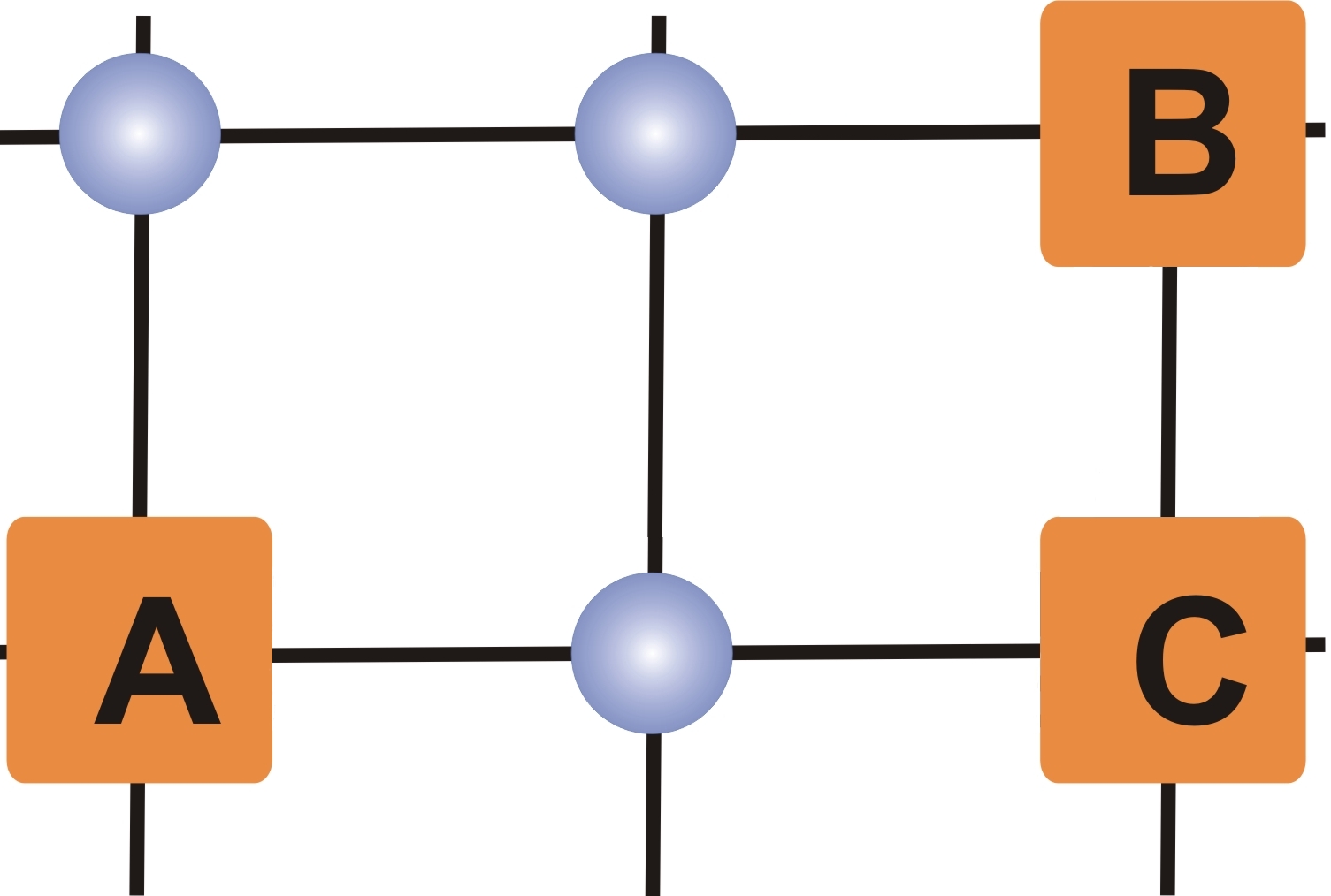
Figure 4: (Color online) Cluster of a term with an extension of 3. The term consists of the operators A,B and C. The taxi cab distance between the outermost operators A and C determines its extension.

To limit the number of generated terms in the course of the flow we define a maximum extension. For each normal-ordered term generated by the commutator the extension is determined. A term with an extension higher than the defined maximum extension is neglected. A CUT truncated to a maximum extension of two only considers terms whose clusters have an extension two or less. (see Fig. 5).

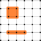
Figure 5: (Color online) The maximum clusters occurring in a calculation with a maximum extension 2. In the following we will call the calculation based on this truncation the plaquette calculation.

In this way more and more extended truncation schemes are used until the numerical results do not change noticeably anymore. Then the calculation is sloppily said to be ‘converged’. To illustrate how the couplings change under the influence of different truncation schemes we consider the nearest-neighbor magnetic exchange constant $J_{1}$

$$H_{\text{Heisenberg}}=J_{1}\sum_{\langle i,j\rangle}\vec{S}_{i}\vec{S}_{j}.$$ (12)

In leading perturbation order one obtains $J_{1}^{(2)}=\frac{4t^{2}}{U}$ Harris and Lange (1967); Takahashi (1977); MacDonald et al. (1988). The results for this coupling constant obtained by CUT are shown in Fig. 6.

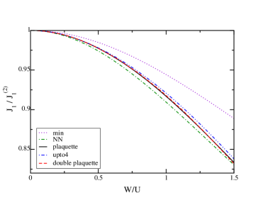
Figure 6: (Color online) Effective nearest-neighbor Heisenberg exchange $J_{1}$ obtained in various truncation schemes relative to the leading perturbative result in $t/U$.

The results are shown for various truncation schemes, where ‘min’ denotes the minimal model in which only the Heisenberg exchange term is kept in addition to the terms present in the initial Hamiltonian. The NN truncation represents a nearest-neighbor calculation defined by the maximum extension 1. This calculation reproduces the second order perturbative result for $J_{1}$. The plaquette calculation contains all terms which fit on the clusters shown in Fig. 5. This truncation corresponds to a maximum extension 2. It reproduces $J_{1}$ up to fourth order in $t/U$.

A maximum extension of 3 corresponds to the so-called ‘double plaquette’ calculation. This truncation scheme is sufficient to describe 6th order processes of $J_{1}$. Since the double plaquette calculation results in a large number of terms an additional truncation scheme is introduced, the ‘upto4’ truncation. In this calculation a subset of processes with extension 3 are considered which consist at most of 4 non-trivial local operators on different sites.

From the results for $J_{1}$ we deduce that $J_{1}$ already converged for a maximum extension 2. Thus the terms contained in a plaquette calculation are sufficient to describe the nearest-neighbor exchange appropriately. Considering even more extended terms does not change the result significantly.

We emphasize that the calculation with a truncation according to the extension is not equivalent to a finite-size cluster calculation. The latter acts on a finite cluster with finite Hilbert space only. The former only restricts the maximum range of physical processes but remains a calculation on the thermodynamic, infinitely large system. The latter computes quantities on finite clusters and a second approximation, for instance finite-size scaling, is needed to extend these finite-cluster results to the infinite system.

III.4 Implementation: Flow Equations

The choice of a truncation scheme implies that the set of differential equations describing the flow is finite. Hence, two tasks have to be accomplished, both of which are implemented on computers. First, the flow equations have to be set up. Even though the large number of running coupling constants makes the use of computer aid indispensable, this step is an essentially analytic calculation. Second, the flow equations are integrated numerically which results in the effective coupling constants determining the effective model. In the effective model the most important subspaces, subspaces of different number of DOs, are decoupled from the rest of the Hilbert space. Thus important observables can be calculated with less effort.

The derivation of the flow equation is realized by a program implemented in C++. This program performs the calculation of the commutators and collects all contributions to the same term. Due to the vast amount of terms it is advantageous to use symmetries to increase the efficiency. If a particular term can be generated from another term by applying symmetry transformations both terms have the same prefactor. The model under study displays the SU(2) spin rotation symmetry and the point group symmetry of the square lattice. This group contains rotation symmetries about $\pi/2$, $\pi$ and $3/2\pi$, reflection symmetries about $x$, $y$ and the diagonal. In the half-filled case the particle-hole symmetry may be used additionally. Of the spin rotation symmetry we only exploited the spin flip symmetry, i.e., the U(1) symmetry of rotations around $S_{z}$. In addition, we used that the Hamiltonian is hermitian conjugate so that adjoint terms also must have the same prefactor.

By applying the above symmetries up to 64 terms are created out of a single term. Since they all carry the same prefactor it is sufficient to treat one representative instead of all 64 terms separately. By this technique, the number of terms is reduced from more than 1.6 million to 26251 in the double plaquette calculation. Yet the double plaquette calculation remains costly. It requires 14.7 weeks of CPU time and more than 20 GB RAM memory.

Compared to the derivation of the flow equations the solution of them is straightforward. We start at $\ell=0$ with the initial Hamiltonian and integrate the differential equations. At $\ell=\infty$ the effective model is reached. Since the integration is performed numerically, this limit can not be reached and we stop before at large enough values of $\ell$.

In order to have a measure to which extent the CUT is accomplished we introduce the residual off-diagonality (ROD) Fischer et al. (2010). The name is motivated by the idea that the CUT eliminates the off-diagonal terms. As we will see in the next subsection the precise choice which terms are eliminated and which are not depends on the choice of the generator $\eta$. Hence in practice the ROD is a measure of the norm of the generator. The ROD is calculated by squaring the (real) prefactors of the terms of the generator, summing them and finally taking the square root of this sum.

The ROD measures to what extent the terms in the generator are eliminated at the current value of the flow parameter $\ell$. When the ROD vanishes, the generator vanishes and consequently the transformation is finished. When the ROD is decreased to some small value, for instance $10^{-15}$, the calculation can be stopped at $\ell<\infty$. The contributions of the remaining off-diagonal terms are negligible so that we consider the model obtained to be the wanted effective model.

III.5 Various Choices of the Generator

Because the number of generated terms during the flow leads to computational costly calculations, we consider various choices of generators for simplification Fischer et al. (2010). The basic idea of the modified generators is that the most relevant physics requires only a very small number of DOs. Hence it may be sufficient to separate subspaces with zero or one DO from the remaining Hilbert space instead of applying $\eta_{\text{pc}}$ which eliminates all terms changing the number of DOs.

An obvious example is the derivation of the Heisenberg model describing the magnetic degrees of freedom without any charges. Here the separation of the subspace without any DO from the remaining Hilbert space is completely sufficient. Thus we consider the generator $\eta_{\text{gs}}$ Fischer et al. (2010)

$$\eta_{\text{gs}}(\ell)=2\sum_{i>0}^{N}\left(\hat{H}_{0}^{i}(\ell)-\hat{H}_{i}^{0}(\ell)\right)$$ (13)

where $N$ denotes the number of quasiparticles. The operator $\hat{H}_{j}^{i}(\ell)$ represents all terms which contain $j$ annihilation operators of DOs and $i$ creation operators of DOs. This generator contains all terms which couple to the subspace without DOs. Note that this subspace is a high-dimensional subspace and not a single ground state for the model under study in contrast to the situation considered by Fischer et al. Fischer et al. (2010). But the other conceptual points, e.g., concerning the formulation in second quantization and the differences to a matrix formulation Dawson et al. (2008) are the same. The Hamiltonian and its evolution under the CUT induced by the gs-generator (13) is graphically represented in Fig. 7.

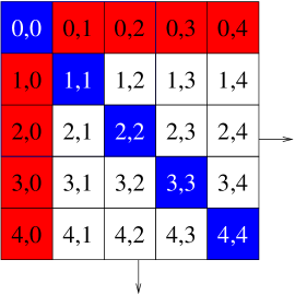
$\Rightarrow$

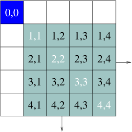
Figure 7: (Color online) Effect of the gs-generator. The terms of the Hamiltonian are labelled according to the number of creation and annihilation operators they contain. Thus a term in the $\left\{i,j\right\}$ block creates $i$ DOs after annihilating $j$ DOs.

If in addition we aim at an explicit description of the motion of a single DO the generator $\eta_{gs,1p}$ has to be used

$$\eta_{\text{gs,1p}}(\ell)=$$ (14)

$$2\sum_{i>0}^{N}\left(\hat{H}_{0}^{i}(\ell)-\hat{H}_{i}0(\ell)\right)+2\sum_{i>0}^{N}\left(\hat{H}_{1}^{i}(\ell)-\hat{H}_{i}1(\ell)\right).$$

In this generator the idea of decoupling some subspaces from the remainder of the Hilbert space is extended to the subspace with one DO. Thus also terms coupling to this subspace are included as depicted in Fig. 8. Whereas the subspaces with zero and with one DO are decoupled at the end of the transformation, the other subspaces are still coupled. To compute eigenvalues in the subspaces of zero or one DO only these subspaces need to be taken into account. In contrast, eigenstates involving two or more DOs still require the diagonalization of the full Hilbert space.

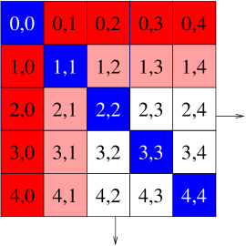
$\Rightarrow$

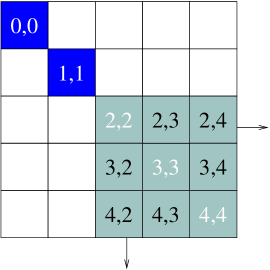
Figure 8: (Color online) Effect of the gs,1p-generator. The terms of the Hamiltonian are labelled according to the number of creation and annihilation operators they contain. Thus a term in the $\left\{i,j\right\}$ block creates $i$ DOs after annihilating $j$ DOs.

The CPU time needed for a double plaquette calculation using various generators are given in Tab. 2. In the case of a CUT based on the gs,1p-generator the use of symmetries is even more efficient. Using all of them except for the particle-hole symmetry reduces the number of terms from 5 million to 55049. The reader may be surprised that these numbers are larger than those for the particle-conserving $\eta_{\text{pc}}$ although terms linking subspaces with higher number of DOs are not decoupled. The explanation is that $\eta_{\text{pc}}$ has the additional feature that it preserves the block-banded structure of the Hamiltonian while the other generators do not Mielke (1998); Knetter and Uhrig (2000); Fischer et al. (2010). Yet the modified generators induce a simpler and faster CUT as shown by the numbers in Tab. 2.

pc-generator	gs,1p-generator	gs-generator
102 days	51 days	less than 10 days

Table 2: Comparison of CPU time needed for a double plaquette calculation using all symmetries in the half-filled case with different generators.

IV Minimal and Nearest Neighbor Model

In this section we present analytic solutions of the flow equations which are possible for the two simplemost truncation schemes. Due to the simplicity of the truncation schemes no difference between the different choices of the generator are found. For concreteness, we consider the particle-conserving $\eta_{\text{pc}}$ here.

IV.1 Minimal Model

The calculation of the minimal model starts by studying all processes on between adjacent sites. This nearest neighbor (NN) calculation is equivalent to a maximal extension of $e=1$. To arrive at the minimal model all terms not present in the initial Hamiltonian except the NN Heisenberg exchange are neglected.

The initial generator takes the form

$$\eta(\ell)=\left[\hat{D},\hat{H}(\ell)\right]=2\hat{T}_{+2}-2\hat{T}_{-2}$$ (15)

with the flow parameter $\ell$. Inserting this definition in the flow equation (3) we calculate

$$\frac{d}{d\ell}H(\ell)=\left[\eta(\ell),\hat{H}_{U}(\ell)+\hat{H}_{t}(\ell)\right].$$ (16)

From the commutator new terms arise Hamerla et al. (2010). In the minimal model all terms except the NN Heisenberg exchange

$$H_{\text{Heisenb.}}=J_{1}(\ell)\sum_{\langle i,j\rangle}\vec{S}_{i}\vec{S}_{j}$$ (17a)

$$\vec{S_{i}}\vec{S_{j}}=\frac{1}{2}\left(\sigma_{i}^{+}\sigma_{j}^{-}+\sigma_{i}^{-}\sigma_{j}^{+}\right)+\frac{1}{4}\sigma_{i}^{z}\sigma_{j}^{z}$$ (17b)

are omitted. The coupling constant $J_{1}(\ell)$ starts at $J_{1}(0)=0$ because it is not part of the initial Hamiltonian $H(0)$. For $\ell\neq 0$ it evolves according to the flow equation.

In this simple case the flow equation can be solved analytically for a general lattice with coordination number $z$ Hamerla et al. (2010). For $\ell=\infty$ the effective model is reached. The effective coupling constants take the form

$$t_{0,\text{eff}} =t_{0}$$ (18a)

$$t_{+2,\text{eff}} =0$$ (18b)

$$U_{\text{eff}} =\frac{1}{2}\sqrt{4U_{0}^{2}+16zt_{0}^{2}}$$ (18c)

$$J_{1,\text{eff}} =\frac{1}{z}\sqrt{4U_{0}^{2}+16zt_{0}^{2}}-\frac{2}{z}U_{0}.$$ (18d)

To obtain the equations for the square lattice $z=4$ must be inserted. The variables $t_{0}$ and $U_{0}$ represent the initial, unrenormalized values of the hopping and the Hubbard repulsion. For simplicity we will omit the subscript 0 and label the unrenormalized values by $t$ and $U$ henceforth. Since the terms $T_{+2}$ and $T_{-2}$ are hermitian conjugates and we assume their coefficients to be real $t_{+2}=t_{-2}$ holds. From (18b) we see that the terms contained in $T_{+2}$ and $T_{-2}$ are eliminated as it should be because they change the number of DOs. The effective model is eventually given by

$$\hat{H}_{\text{eff}}=U_{\text{\text{eff}}}\frac{1}{2}\hat{D}+\hat{T}_{0}+J_{1,\text{eff}}\sum_{<i,j>}\vec{S_{i}}\vec{S_{j}}\,.$$ (19)

IV.2 Nearest Neighbor Model

In the nearest neighbor model all terms arising from a nearest neighbor calculation are included in the effective model as well as in the generators. This is the full calculation with extension 1. It can still be solved analytically Hamerla et al. (2010). In this truncation scheme the Heisenberg exchange coupling is given by

$$J_{1,\text{eff}}=\frac{2}{3+z}\left(\sqrt{U_{0}^{2}+4(3+z)t_{0}^{2}}-U_{0}\right).$$ (20)

Note the differences to the result of the minimal model (18d). Of course, this differences arises only beyond leading order.

Besides the Heisenberg exchange the calculation contains the term $\hat{H}_{V}$ describing the interaction of two DOs

$$\hat{H}_{V}(\ell)=V(\ell)\sum_{<i,j>}\bar{n}_{i}\bar{n}_{j}.$$ (21)

The operator $\bar{n}$ counts the amount of electrons compared to the mean value of the filling. For the half-filled case the mean value is $1$.The third term created during the flow is

$$\hat{H}_{p}(\ell)=V_{p}(\ell)\sum_{<i,j>}\left(\hat{c}_{i\uparrow}^{\dagger}\hat{c}_{i\downarrow}^{\dagger}\hat{c}_{j\downarrow}^{\phantom{\dagger}}\hat{c}_{j\uparrow}^{\phantom{\dagger}}+\text{h.c.}\right)\,.$$ (22)

describing pair hopping processes of DOs. One of the processes contained in this term is the hopping of two electrons from site $j$ to an empty site $i$. As the empty state as well as the doubly occupied state represents a DO this process does not change the number of DOs. In the effective model $V$ and $V_{p}$ take the values

$$V_{\text{eff}} =-\frac{2}{3+4z}\sqrt{U2+4(3+z)t2}+\frac{2}{3+4z}U_{0}$$ (23a)

$$V_{p,\text{eff}} =\frac{4}{3+4z}\sqrt{U2+4(3+z)t2}+\frac{4}{3+4z}U_{0}.$$ (23b)

In the case of doping another contribution to the flow equation also arises. It reads

$$\hat{H}_{\mu} =\mu\sum_{i}\bar{n}_{i,\delta}$$ (24)

and determines the chemical potential $\mu$. In the effective model this constant takes the value

$$\mu_{\text{eff}} =\frac{\delta z}{2(3+z)}U\sqrt{1+4(3+z)\frac{t^{2}}{U^{2}}}-\frac{z}{2(3+z)}U\delta\,.$$ (25)

with the coordination number $z$. In leading order in $\frac{t}{U}$ this yields a chemical potential which depends linearly on the doping constant $\delta$ and on the coordination number of the lattice

$$\mu^{(2)}=\delta z\frac{t^{2}}{U}\,.$$ (26)

V Influence of the Choice of Generator

In this section the influence of the choice of the generator is studied. First, we consider the ROD defined in Sect. III for the gs-generator (13), gs,1p-generator (14), and the pc-generator (8). The results for the ROD obtained in a double plaquette calculation at half-filling are shown in Fig. 9 as functions of the continuous flow parameter $\ell$.

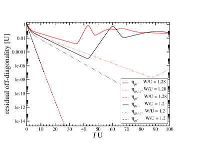
Figure 9: (Color online) Behavior of the residual off-diagonality (ROD) in a double plaquette calculation for various choices of the generator for various initial ratios $W/U$.

For the gs-generator, the ROD converges for all values of the ratio $W/U$. In contrast, the ROD for the gs,1p-generator and even more pronounced the ROD for the pc-generator show non-monotonic behavior for larger values of $W/U$.

Non-monotonic behavior of the ROD suggests that the intended transformation does not succeed. There is no strict statement that a successful CUT has to have a monotonic ROD. It is well possible that the ROD displays local maxima which indicate that some energy eigenstates are re-ordered, see for instance Ref. Dusuel and Uhrig, 2004. If the CUT is performed without approximation any unitary transformation is as good as any other. But since we have to truncate many terms the upturn of the ROD indicates a potential loss of accuracy. If the total norm of the off-diagonal terms is large there is still a significant transformation to be done. In the course of this transformation the truncation of terms may introduce significant errors. In return, a quickly decreasing ROD indicates that all coefficients to be eliminated decay fast and significant truncation errors are less likely. But we like to stress that the behavior of the ROD is only an indicator for possible truncation errors which eventually may imply that the intended mapping breaks down.

The faster convergence of the gs-generator is straightforward to understand because the gs-generator comprises only terms which create DOs from the reference ensemble or which annihilate them, see Eq. (13) and Fig.  7. As long as there is a finite charge gap $\Delta_{g}$ these processes are exponentially suppressed: $\propto\exp(-\Delta_{g}\ell)$. For the gs,1p-generator the processes starting from one DO creating two additional DOs can be more difficult to suppress if they decrease the total energy. This is possible if the DOs disperse and a DO at high energies decays into three DOs at lower energy.

The pc-generator aims in addition at eliminating processes starting from two and more DOs so that there are even more processes which may decrease the total energy while the number of DOs increases. Hence we are not surprised to see that the pc-generator induces a flow of the ROD which displays even more pronounced non-monotonic behavior.

From these observations the conclusion to always favor the gs-generator suggests itself. But it is in fact a trade-off. The gs-generator is quicker to implement and more robust in its convergence, but it achieves less because it decouples only the subspace without any DOs. For deriving only an extended Heisenberg model this is completely sufficient and hence for this aim the gs-generator is the generator of choice. But if one is additionally interested in an explicit description of the dynamics of DOs the other generators are advantageous as we will illustrate next.

To see how the coupling constants are influenced by the choice of generator a few exemplary results are shown. One of the most important magnetic coupling constants besides the nearest neighbor coupling $J_{1}$ is the Heisenberg interaction between next-nearest neighbors $J_{2}$, i.e., diagonal over a plaquette. The behavior of this exchange coupling as function of $W/U$ for the three generators is depicted in Fig. 10.

Figure 10: (Color online) Behavior of the next nearest neighbor interaction $J_{2}$ for different generators as function of $W/U$ determined in an upto4 calculation. The results for the three generators almost coincide even for large values of $W/U$.

The curves for all three generators almost coincide. This underlines that it is completely sufficient to use the gs or the gs,1p-generator for the determination of this coupling. All processes contributing to this coupling are included in the CUT induced by the gs-generator. This can be understood from the fact, that the magnetic coupling $J_{2}$ describes an interaction within the subspace of half-filled states, i.e., the subspace without any DO. This subspace is decoupled from the remainder of the Hilbert space by all three generators. If no truncation errors occurred, all three generators would indeed yield precisely the same result, cf. Ref. Fischer et al., 2010.

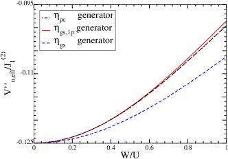
Figure 11: (Color online) Density-density interaction between third nearest neighbors for different generators obtained in an upto4 calculation. The results for the $pc$- and the $gs,1p$-generator agree very well whereas the results of $gs$-generator show larger deviations.

In contrast to a pure spin-spin coupling the term

$$\hat{H}_{Vn}^{\prime\prime} =V^{\prime\prime}_{n}\sum_{\alpha,\beta}\sum_{\langle\langle i,j\rangle\rangle}\left\{\left(1-\hat{n}_{i,\alpha}^{\phantom{\dagger}}\right)\hat{c}_{i,\bar{\alpha}}^{\dagger}\hat{c}_{j,\bar{\beta}}^{\phantom{\dagger}}\left(1-\hat{n}_{j,\beta}^{\phantom{\dagger}}\right)\bar{n}_{k}\right.$$

$$\left.+\hat{n}_{i,\alpha}^{\phantom{\dagger}}\hat{c}_{i,\bar{\alpha}}^{\dagger}\hat{c}_{j,\bar{\beta}}^{\phantom{\dagger}}\hat{n}_{j,\beta}^{\phantom{\dagger}}\bar{n}_{k}+\text{h.c.}\right\}.$$ (27)

acts on two DOs. It describes the hopping of an electron from a singly occupied site to an empty site under the condition that site $k$ is occupied by a DO. It is a process which is not active on the subspace with zero or only one DO. We do not expect that the results for the different generators agree. Indeed, the results for this coupling constant (Fig. 11) show rather large deviations of the results obtained by the gs-generator from the results obtained by the other two generators. This illustrates that the gs-generator induces a different unitary transformation than the other two generators. Note that the deviations do not necessarily imply that the gs-result is less accurate because it results from the representation of the Hamiltonian in a different basis.

In view of the above arguments, it is surprising that the results of the gs,1p-generator and the pc-generator are so close to each other. From their definitions we expect that the pc- and the gs,1p-results agree very well for processes involving a single DO, but not necessarily for processes involving two DOs.

In conclusion, the question which generator is optimum cannot be answered generally. It depends on the particular objective of the intended investigation.

VI apparent charge gap

In the previous sections we have started to discuss the issue for which conditions the intended mapping from the Hubbard model to a generalized $t$-$J$ model is possible and justified. Qualitatively it is obvious that $U$ must be large enough. But quantitative indicators are needed. Here we aim at giving a quantitative estimate for the parameter range in which the mapping is justified.

VI.1 General Considerations

The basis of the transformation from the Hubbard model to the $t$-$J$ model is the elimination of charge fluctuations. These charge fluctuations correspond to changes in the number of DOs. The corresponding processes are the ones that we consider to be off-diagonal. To be able to eliminate such processes the subspaces with differing numbers of DOs have to be separated in energy. In Sect. III we introduced the residual off-diagonality (ROD) as a measure to decide if for a given $\ell$ the off-diagonal terms are small enough to be neglected.

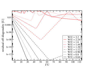
Figure 12: (Color online) Behavior of the residual off-diagonality (ROD) for the pc-generator obtained in a double plaquette calculation for different values of $W/U$. The ROD measures to which extent charge fluctuations are eliminated as function of the flow parameter $\ell$.

Figure 12 shows the behavior of the ROD of the pc-generator for the double plaquette calculation at various values of $W/U$. For small values of the flow parameter $\ell U<2.24$ the ROD decreases exponentially. If the ratio $W/U$ is increased to $W/U=1.12$ the ROD evolves non-monotonically. For $\ell U<64$ the ROD falls below $10^{-13}$ to rise again for larger values of $\ell$. For even higher values of $W/U$ this increase sets in for smaller and smaller $\ell$.

We argued in the preceding section that a non-monotonic behavior of the ROD as observed in Fig. 12 is a first clue for a possible breakdown of the mapping. Although the non-monotonicity indicates problems of the mapping already for $W/U=1.12$ no sign of a possible breakdown can be seen in the coupling constants, see for instance Fig. 10. This is due to the fact, that the dominant spin coupling constants are already converged to their value in the effective model for small values of $\ell$. Thus processes appearing only at large $\ell$ have no influence on these values.

To make progress in determining the range of validity of the mapping we have to study the separation of energy scales between the states without DOs and the states with DOs. To this end we investigate the energies of an added electron or an added hole to the system, that means the density-of-states (DOS) which comprises the LHB and the UHB for large $U$, see Figs. 1 and 2. If $W$ is increased the bands approach each other and eventually touch so that there is no energy separation anymore. States with differing number of DOs have the same energy so that charge fluctuations can not be eliminated. In a paramagnetic description by dynamic mean-field theory (DMFT) the Mott-insulating phase becomes unstable at this very point Georges et al. (1996); Nishimoto et al. (2004); Garcia et al. (2004); Karski et al. (2005).

Turning the argument around we use the gap $\Delta_{g}$ between the lower and the upper Hubbard band as quantitative indicator of the energy separation of subspaces with different number of DOs. If $\Delta_{g}$ is finite there is good physical reason to regard the mapping of the Hubbard model onto the $t$-$J$ model as justified. If $\Delta_{g}$ vanishes the mapping has to break down.

There is one additional aspect to which we have to draw the reader’s attention. In infinite dimensions, where DMFT is exact, one may suppress long-range magnetic order and consider the paramagnetic phase which does not show an spin-spin correlation between different sites so that the insulating paramagnetic phase behaves like the reference ensemble (9) for $\delta=0$. In particular, the charge gap does not depend on the spin state.

But in finite dimensions, even without long-range magnetic order one has to expect that the charge gap will generically depend on the spin state. Hence there is no well-defined charge gap without specifying the state of the spin degrees of freedom. Thus we have to introduce the concept of the apparent charge gap $\Delta_{g}$ Reischl et al. (2004) which is designed to describe the energy separation of subspaces with different number of DOs if an electron is added to the disordered reference ensemble (9). The apparent charge gap is not rigorously defined and it cannot be measured precisely in experiment because it does not capture bandtails of the Hubbard bands which carry little spectral weight. But it is an estimate for the energy separation between states without DOs and states with DOs. Hence it provides an appropriate estimate of the range of validity of the mapping from the Hubbard model to the $t$-$J$ model.

We calculate $\Delta_{g}$ for the effective $t$-$J$ model derived before. In the half-filled case the gap is calculated by estimating the lowest possible energy of an added DO, for details see below. Calculations for the half-filled case indicate a closure of the gap for $W/U\approx 0.9$ Reischl et al. (2004). In the doped case the calculation of $\Delta_{g}$ is divided into two steps as can be understood from the DOS sketched in Fig. 2.

To calculate the apparent gap we first determine the lowest possible energy $\Delta_{\text{UHB}}$ of a DO in the upper Hubbard band. In a second step we calculate the maximum energy for the destruction of a DO $\Delta_{\text{LHB}}$, that means for adding an electron to an empty site. Hence in the doped case we use

$$\Delta_{g}=\Delta_{\text{UHB}}-\Delta_{\text{LHB}},$$ (28)

while in the undoped case we have

$$\Delta_{g}=2\Delta_{\text{UHB}}.$$ (29)

Note that the seemingly discontinuous definition of $\Delta_{g}$ as function of $\Delta_{\text{UHB}}$ stems from the discontinuous evolution of the Fermi level which jumps upon hole doping from the middle between the Hubbard bands to the edge of the lower Hubbard band.

VI.2 Calculation of $\Delta_{g}$

The apparent charge gap is calculated for the effective $t$-$J$ model. A full diagonalization of the Hamiltonian is not feasible and it would not provide what we need, namely the charge gap above the disordered reference ensemble (9). Hence we apply a Lanczos approach in terms of operators. The Lanczos approach is appropriate because we only aim at extremum eigenvalues. Since we have to deal with operators acting on the reference ensemble Reischl et al. (2004), which is a mixed state, the Liouville formulation of this method has to be used Mori (1965); Fulde (1993); Viswanath and Müller (1994). The evolution of an operator $\hat{A}$ is given by the Liouville superoperator

$$\mathcal{L}\,\hat{A}=\left[\hat{H}_{\text{eff}},\,\hat{A}\right]\,.$$ (30)

The effect of this superoperator applied to the creation operator of a DO consists of moving the DO and changing the spin background. With this operator a basis of operators $\left\{\hat{v}_{0},...\hat{v}_{n}\right\}$ describing the DO with momentum $k$ and the effect on its surrounding spins is built recursively. In the first part of the calculation the minimal energy of a DO with momentum $k$ is calculated. The calculation starts with the vector

$$\hat{v}_{0}=\frac{1}{\sqrt{N}}\sum_{\vec{r}}e^{i\vec{k}\vec{r}}\hat{n}^{\phantom{\dagger}}_{\vec{r},\downarrow}\,\hat{c}^{\dagger}_{\vec{r},\uparrow}\,.$$ (31)

where $N$ denotes the number of lattice sites and the vector $\vec{r}$ determines the actual position of the DO. The action of this operator is to put an $\uparrow$ electron on a site which is already occupied by a $\downarrow$ electron so that a doubly occupied site is created. From this starting vector the basis is built recursively by

$$\hat{v}_{i+1}=\mathcal{L}\hat{v}_{i}-a_{i}\hat{v}_{i}-b_{i}^{2}\hat{v}_{i-1}$$ (32)

according to the rules of the Lanczos tridiagonalization. The scalar product of the Liouville formulation Fulde (1993) is defined as

$$\left(\hat{A}|\hat{B}\right)=\text{Tr}\left(\hat{A}^{\dagger}\hat{B}^{\phantom{\dagger}}\hat{\rho}_{0}^{\phantom{\dagger}}\right)\,.$$ (33)

with the statistical operator $\hat{\rho}_{0}$ of the reference ensemble (9). The prefactors $a_{i}$ are given through the projection onto $\hat{v}_{i}$

$$a_{i} =\frac{\left(\hat{v}_{i}|\mathcal{L}\hat{v}_{i}\right)}{\left(\hat{v}_{i}|\hat{v}_{i}\right)}$$ (34)

and the $b_{i}$ are given by

$$b_{i}^{2}=\frac{\left(\hat{v}_{i}|\hat{v}_{i}\right)}{\left(\hat{v}_{i-1}|\hat{v}_{i-1}\right)}\,.$$ (35)

In this operator basis the Liouville superoperator takes tridiagonal form with the coefficients $a_{i}$ on the diagonal the coefficients $b_{i}$ on the secondary diagonals.

If infinitely many iterations were performed the dispersion of a DO relative to the disordered spin background would be given as the lowest energy in the subspace spanned by the calculated operator basis. In real calculations only a few iterations are feasible due to the humongous number of terms in the effective Hamiltonian. Starting with the vector $\hat{v}_{0}$ in (31) consisting of one single operator, the commutation leads to increasingly complicated terms whose appropriate superposition describes $\hat{v}_{j}$. The effort grows exponentially with the number of iterations. Thus we restrict ourselves to a finite basis $\left\{\hat{v}_{0}\ldots\hat{v}_{n}\right\}$. The lowest energy calculated in the subspace spanned by $\left\{\hat{v}_{1}\ldots\hat{v}_{n}\right\}$ yields an upper bound $\Delta_{\text{UHB}}$ to the real dispersion of the DO. Note that in the following we denote by $\Delta_{\text{UHB}}$ this upper bound in order to keep the notation simple.

In the half-filled case the apparent charge gap results from Eq. (29). For finite doping the particle-hole symmetry is lost, the Fermi energy jumps to the LHB, and the value $\Delta_{\text{LHB}}$ has to be determined. To this end, we start from the modified vector

$$\hat{u}_{0}=\frac{1}{\sqrt{N}}\sum_{\vec{r}}e^{i\vec{k}\vec{r}}\hat{c}^{\dagger}_{\vec{r},\uparrow}\left(1-\hat{n}^{\phantom{\dagger}}_{\vec{r},\downarrow}\right).$$ (36)

This operator destroys a DO by placing a single electron on an empty site. The value for $\Delta_{\text{LHB}}$ we obtain from the calculation in a finite subspace $\left\{\hat{u}_{0}\ldots\hat{u}_{n}\right\}$ is a lower bound to the true maximum energy. Finally the apparent charge gap is given by (28) in dependence on the doping level $\delta$. As argued before the mapping to the $t$-$J$ model is justified as along as $\Delta_{g}\geq 0$.

Extremum values of $E_{k}$ occur at the high symmetry points of the Brillouin zone. Thus we avoid costly calculation of the whole dispersion and focus on the momenta $\vec{k}=\left(0,0\right)$ and $\vec{k}=\left(\pi,\pi\right)$ where the lattice constant is set to unity. The calculations rely on the the nearest neighbor effective model. Previous calculations in the half-filled case Reischl et al. (2004) showed that there is no significant change in the results obtained for different truncation schemes because the main uncertainty results from the limited number of iterations in the Lanczos tridiagonalization. The truncation of the effective model used plays only a minor role. Since only a few iterations were feasible we additionally perform an extrapolation. The results for the gaps are extrapolated in $1/n$ with $n$ denoting the number of iterations. By extrapolating to $n=\infty$ we obtain an estimate for $\Delta_{g}$; for more details we refer to Ref. Reischl et al., 2004. Figure 13 displays the extrapolation for the half-filled case. For the doped case, $\Delta_{\text{LHB}}$ and $\Delta_{\text{UHB}}$ are extrapolated separately in $1/n$.

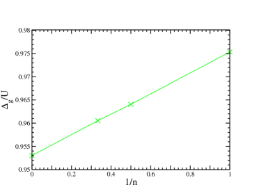
Figure 13: (Color online) Linear extrapolation in $\frac{1}{n}$ of the apparent charge gap at half-filling for $W/U=0.5$ obtained by $n$ iterations.

VI.3 Results for $\Delta_{g}$

The apparent charge gap is computed for the effective $t$-$J$ model derived by a CUT with NN truncation using the pc-generator or the gs,1p-generator. The gs-generator is not used in this context because the resulting effective model mixes a single DO with the subspaces of two and more DOs. The gap is calculated for various doping levels as function of $W$. Thus the value $W/U$ up to which the mapping is justified is estimated from $\Delta_{g}(W/U)=0$. The minimum $\Delta_{\text{UHB}}$ of the dispersion of a DO is found for a vanishing momentum. The maximum energy $\Delta_{\text{LHB}}$ for the destruction of a hole is found for a momentum $\vec{k}=\left(\pi,\pi\right)$.

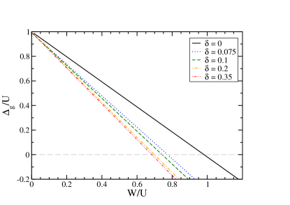
Figure 14: (Color online) The extrapolated apparent charge gap as function of $W/U$ for various $\delta$.

The results for the extrapolated $\Delta_{g}$ are displayed in Fig. 14 for various values of the doping $\delta$. For vanishing bandwidth $W=0$ the apparent gap is given by the Hubbard repulsion $U$. Thus the curves of $\Delta_{\text{app}}/U$ start at unity. Then the gap decreases almost linearly until $\Delta_{\text{app}}=0$ is reached. Negative values of the gap indicate the breakdown of the mapping. The linear decrease of the gap has also been observed for the half-filled case Gebhard (1997). The decrease leads to a closure of the charge gap for $W/U=1$. For the Bethe lattice with $z\rightarrow\infty$ a closure of the gap was found for $W/U=0.89$ Nishimoto et al. (2004) which agrees well with our estimate in view of the different lattices and techniques. Other numerical evaluations of DMFT for the Bethe lattice yield a closure of the insulating gap at $W/U\approx 0.84$ Garcia et al. (2004) or at $W/U\approx 0.83$ Karski et al. (2005).

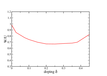
Figure 15: (Color online) Limiting values for $W/U$ up to which a mapping of the Hubbard model to the effective $t$-$J$ model is justified. It is derived from the zeros $\Delta_{g}(W/U)=0$ as function of doping.

Our results indicate that the apparent charge gap $\Delta_{g}$ for the square lattice closes at $W/U\approx 0.98$ for $\delta=0$. Upon doping $\Delta_{g}$ vanishes even faster upon increasing bandwidth so that the range of applicability of the mapping ‘Hubbard model $\to$ $t$-$J$ model’ is reduced. From the values of $W/U$ where $\Delta_{g}$ beomes zero we estimate this range of applicability. The result is shown in Fig. 15 which represents one of the central results of this work. Our approach provides the first systematic derivation of this diagram of applicability as function of doping.

The range of applicability decreases from $W/U\approx 0.98$ for $\delta=0$ to $W/U\approx 0.67$ for $\delta=0.25$. Then the range of applicability increases again slightly to $W/U=0.73$ for $\delta=0.4$. The plateau in $W/U(\delta)$ and the moderate increase are rather unexpected, cf. Ref. Millis and Coppersmith (1991). We do not have an obvious explanation for it. In contrast, the decrease of the range of applicability for $\delta\leq 0.3$ meets the qualitative expectation since a doped system has a higher mobility of charges so that the energy separation of sectors of differing number of DOs becomes smeared out.

The relative constant limiting value for $W/U$ below which the use of a generalized $t$-$J$ model is justified provides interesting information on the applicability of $t$-$J$ models for doped systems. The use of $t$-$J$ models is very widespread in theoretical studies for the high-$T_{c}$ superconductors based on cuprates. Commonly used parameters are $W/U\approx 0.7$ and $\delta<0.3$ Ogata and Fukuyama (2008). Our results indicate that the use of $t$-$J$ models is indeed justified. But caution is required in the doping range $0.18\lessapprox\delta\lessapprox 0.25$ where $W/U\approx 0.7$ is at about the limit of applicability. Thus our results shed light on the important question of the applicability of a commonly used model. It is remarkable that the issue of how to justify this model for significant levels of dopings has attracted so little attention so far.

VII results for the relevant coupling constants

In the preceding section we comprehensively discussed the applicability of the derivation of a generalized $t$-$J$ model. The result of this discussion is summarized in the estimated range of applicability shown in Fig. 15. In the present section, we provide the coupling constants which ensue from the CUT of the Hubbard model to the $t$-$J$ model. Results are given in the range $W/U\leq 1.0$ because the mapping definitely breaks down beyond.

All results shown are derived from upto4 calculations using the pc-generator. Additionally we performed random double plaquette calculations with the gs,1p-generator to check if there are changes in the coupling constants when higher truncation schemes are applied. No significant differences are found. Thus the upto4 truncation appears to be sufficient to determine the coupling constants. The results for the half-filled case ($\delta=0$) shown in the following figures agree perfectly with the results obtained by Reischl et al. Reischl et al. (2004).

Although the mapping generates a large number of terms, only few of them are really relevant in the final effective model. Most others only have very small prefactors.

VII.1 Chemical Potential

First, we consider the chemical potential as defined in (24). In leading quadratic order of $\frac{t}{U}$ it is proportional to $\delta$. Therefore $\mu$ will be shown in units of $\delta J_{1}^{(2)}$ as defined in (12). The ratio $\mu/\delta$ shows almost no dependence on $\delta$, see Fig. 16. As function of $W/U$ the chemical potential stays rather constant and even for $W/U=1$ the deviations are small. The dependence on $W/U$ is greater for smaller values of $\delta$ concentration.

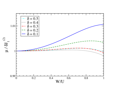
Figure 16: (Color online) Chemical potential relative to $\delta J_{1}^{(2)}$for various doping concentrations $\delta$.

VII.2 Spin Terms

The dominant terms of the effective model are the Heisenberg-type spin interactions.

$$H_{\text{Heisenb.}|i-j|}=\sum_{i,j}J_{|i-j|}\vec{S}_{i}\vec{S}_{j}\,.$$ (37)

The largest contribution of this type is the Heisenberg exchange $J_{1}$ between nearest neighbors. All results are shown relative to the leading perturbative result $J_{1}^{(2)}=\frac{4t^{2}}{U}$.

The left panel of Fig. 17 shows the dependence of $J_{1}$ on the ratio $W/U$. Starting from $J_{1}^{(2)}$ for $W/U=0$ the coupling constant takes slightly smaller values for larger $W/U$. Additionally, the doping dependence of $J_{1}$ for various values of $W/U$ is shown relative to its value for the undoped system in the right panel of Fig. 17. $J_{1}$ increases with $\delta$. The doping has a greater influence for larger values of $W/U$, but the effect remains rather small. Even for $W/U=0.8$ the doping causes a change in $J_{1}$ of only about $3\%$.

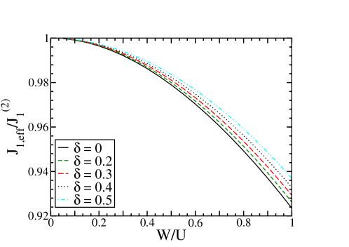
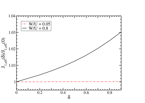
Figure 17: (Color online) Dependence of $J_{1}$ on $W/U$ for various values of $\delta$ (left panel). The dependence on $\delta$ for two ratios $W/U$ is depicted in the right panel. The undoped value for $W/U=0.05$ is found to be $J_{1}(0)\approx 1.5621\cdot 10^{-4}\,U$. For $W/U=0.8$ $J_{1}(0)$ takes the value $0.0379\,U$.

The Heisenberg exchange between next-nearest (diagonal) neighbors $J_{2}$ as well as the exchange $J_{3}$ between neighbors at a linear distance of two lattice spacings are much smaller than $J_{1}$. Both terms appear in fourth order of $\frac{t}{U}$. Even for $W/U=1$ $J_{2}$ is smaller than $0.03J_{1}$, see Fig. 18. Surprisingly, $J_{2}$ shows a slightly more significant (relative) dependence on the dopant concentration than $J_{1}$, see Fig. 18. Yet, in view of the small absolute values of $J_{2}$, this doping dependence can be neglected.

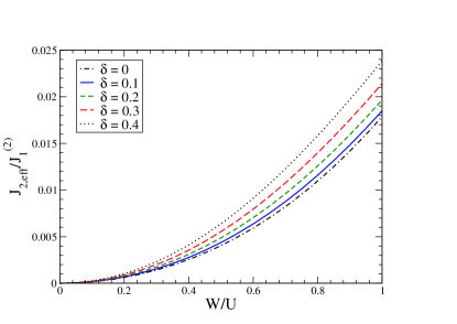
Figure 18: Effective $J_{2}$ for various doping concentrations as function of $W/U$.

As can be seen in the right panel of Fig. 19 the coupling $J_{3}$ shows a counter-intuitive behavior. First it decreases upon doping but increases again beyond $\delta\approx 0.3$.

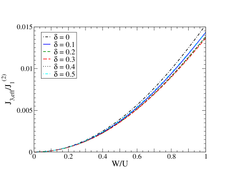
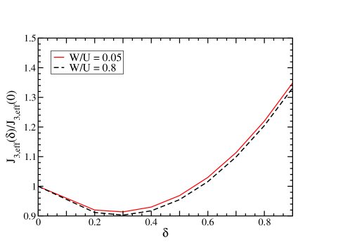
Figure 19: (Color online) Dependence of $J_{3}$ on $W/U$ for various values of $\delta$ (left panel). The dependence on $\delta$ for two ratios $W/U$ is depicted in the right panel. The undoped values are $J_{3}(0)\approx 6.1039\cdot 10^{-9}\,U$ for $W/U=0.05$ and $J_{3}(0)\approx 3.9802\cdot 10^{-4}\,U$ for $W/U=0.8$.

Besides the 2-spin terms in (37) the two dimensional square lattice also allows for 4-spin interactions. The leading contribution is given by

$$\hat{H}_{\Box} =J_{\Box}\sum_{<i,j,k,l>}\left[\left(\vec{S}_{i}\vec{S}_{j}\right)\left(\vec{S}_{k}\vec{S}_{l}\right)+\left(\vec{S}_{i}\vec{S}_{l}\right)\left(\vec{S}_{j}\vec{S}_{k}\right)-\right.$$

$$\left.\left(\vec{S}_{i}\vec{S}_{k}\right)\left(\vec{S}_{j}\vec{S}_{l}\right)\right]$$ (38)

which we sloppily call ring exchange although the complete ring exchange comprises also nearest-neighbor and diagonal 2-spin couplings Brehmer et al. (1999). We do so since these 2-spin terms are accounted for by $J_{1}$, $J_{2}$, and $J_{3}$ in (37). The term (38) describes the interaction of the four spins on a plaquette, see Fig. 20, and it occurs first in order $\left(\frac{t}{U}\right)^{4}$  Takahashi (1977). Its importance is discussed at length in the literature, see for instance. Refs. Schmidt and Kuramoto, 1990; Brehmer et al., 1999; Müller-Hartmann and Reischl, 2002; Katanin and Kampf, 2002; Reischl et al., 2004; Schmidt and Uhrig, 2005 and references therein. The magnetic excitations in planar cuprates may not be understood without considering ring exchange Müller et al. (2004); Lorenzana et al. (1999); Notbohm et al. (2007).

Figure 20: (Color online) Positions of spins interacting via the ring exchange $H_{\Box}$.

Compared to other quartic exchange couplings such as $J_{2}$ or $J_{3}$ the ring exchange is much more important, see its values in Fig. 21. The ring exchange takes values of up to $20\%$ of $J_{1}$. Hence this term must not be neglected in an effective model.

The ring exchange shown in Fig. 21 displays nearly no dependence on the doping $\delta$. Even for doping as large as $\delta=0.8$ the change in the coefficient is less than $1.12$ percent. Thus while ring exchange is an important process its doping dependence can safely be omitted.

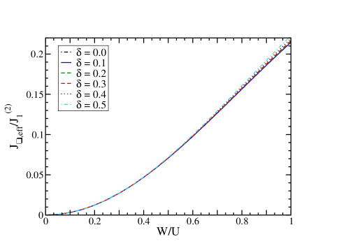
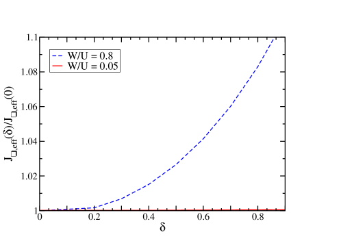
Figure 21: (Color online) Effective ring exchange term $J_{\Box}$ for various values of $\delta$ (left panel) and its doping dependence of $J_{\Box}$ (right panel) relative to the undoped values $J_{\Box}\approx 2.4390\cdot 10^{(}-7)\,U$ for $W/U=0.05$ and $J_{\Box}(0)\approx 0.0125\,U$ for $W/U=0.8$.

The second 4-spin term is the cross exchange

$$\hat{H}_{\times}=J_{\times}\sum_{<i,j,k,l>}\left(\vec{S}_{i}\vec{S}_{k}\right)\left(\vec{S}_{j}\vec{S}_{l}\right).$$ (39)

In this term the spins are located on the same sites as for the ring exchange, but the inner products are taken of the diagonal spins. The corresponding coupling constant is shown in Fig. 22. It takes smaller values than $J_{\Box}$ and hardly shows any doping dependence.

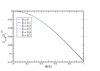
Figure 22: (Color online) Effective $J_{\times}$ as defined in Eq. 39 for various doping concentrations $\delta$.

VII.3 Interaction of Double Occupancies

The effective generalized $t$-$J$ model also contains interactions between DOs. First, we consider the Hubbard repulsion $U$ which determines the energy costs for the creation of a single DO. So strictly speaking it does not represent a true interaction. Since the deviations of the doped values of $U$ from the ones in the half-filled case are small we directly show the doped values relative to the half-filled ones in Fig. 23. This coupling constant shows nearly no dependence on the doping $\delta$. Hence the influence of doping on $U$ may be neglected.

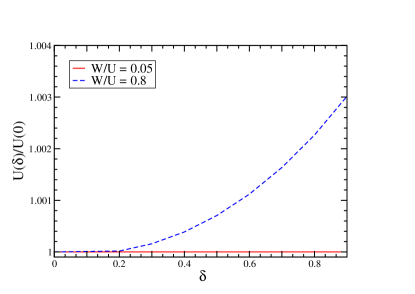
Figure 23: (Color online) Hubbard repulsion for the doped case relative to the value in the half-filled case as function of $\delta$ for various values of $W/U$. The doped values are given relative to the undoped values of $U(0)\approx 1.0003\,U$ for $W/U=0.05$ and $U(0)\approx 1.0787\,U$ for $W/U=0.8$.

The following interaction terms are active only in the presence of at least two DOs. Thus these terms have to be seen as genuine 2-DO interactions. Among them density-density interactions of various distances appear. The density-density interaction between nearest neighbors reads

$$\hat{H}_{V}=V\sum_{<i,j>}\bar{n}_{i,\delta}\bar{n}_{j,\delta},$$ (40)

where $\bar{n}_{\delta}$ denotes the operator counting the number of electrons on a site compared to the average filling, cf. Tab. 1. At half-filling this term only contributes if site $i$ and site $j$ are either empty or truly doubly occupied. Figure 24 only shows an increase in the coupling constant of about $1\%$ under the influence of doping for $W/U=0.8$.

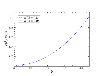
Figure 24: (Color online) Effective density-density interaction as function of doping for various values of $W/U$. Results are given relative to the values at zero doping $V(0)\approx-3.9056\cdot 10^{-5}\,U$ for $W/U=0.05$ and $V(0)\approx-9.2525\cdot 10^{-3}\,U$ for $W/U=0.8$.

A second type of interaction is correlated hopping. The most important term of this kind is the hopping of two electrons to a nearest neighbor site which is initially empty, see Eq. 22. Since the empty state also corresponds to a DO, the effect of the term is to exchange the two DOs. The results for various doping levels are depicted in Fig. 25.

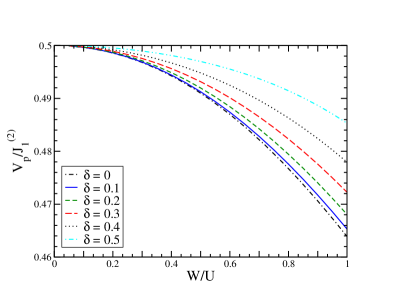
Figure 25: (Color online) Effective pair interaction $V_{p}$ as defined in Eq. 22 for various $\delta$ as a function of $W/U$.

Besides the nearest neighbor pair interaction $V_{p}$ there are also pair interaction terms between three spins. One of these terms is the interaction of three spins on a plaquette which reads

$$\hat{H}^{\prime}_{\text{pair}} =V^{\prime}_{p}\sum_{\sigma}\sum_{<i,j,k>}\left[\hat{c}_{k,\sigma}^{\dagger}\hat{c}_{k,\bar{\sigma}}^{\dagger}\hat{c}_{i,\bar{\sigma}}^{\phantom{\dagger}}\hat{n}_{i,\sigma}^{\phantom{\dagger}}\hat{c}_{j,\sigma}^{\phantom{\dagger}}(1-\hat{n}_{j,\bar{\sigma}}^{\phantom{\dagger}})+\right.$$

$$\left.\hat{c}_{k,\sigma}^{\dagger}\hat{c}_{k,\bar{\sigma}}^{\dagger}\hat{c}_{i,\bar{\sigma}}(1-\hat{n}_{i,\sigma}^{\phantom{\dagger}})\hat{c}_{j,\sigma}^{\phantom{\dagger}}\hat{n}_{j,\bar{\sigma}}+\text{h.c.}\right].$$ (41)

The sites $i$ and $j$ are supposed to be diagonal neighbors with a common adjacent site $k$. One possible process consists of the hopping of an electron from a singly occupied site $j$ to an empty site $k$. Simultaneously, an electron from the doubly occupied site $i$ hops to site $k$ forming a DO on this site. The corresponding effective coupling constant $V^{\prime}_{p}$ is depicted in Fig.  26 as function of doping.

Since this correlated hopping imposes an additional constraint on the state of site $k$ it is half as large as the nearest neighbor term $V_{p}$. Even for large values of $W/U$ the coupling constant is increased only by $8\%$ for large doping.

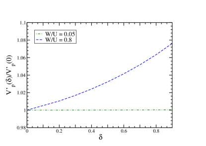
Figure 26: (Color online) Effective pair interaction $V_{p}^{\prime}$ on $W/U$ for various $\delta$. In the undoped case $V^{\prime}_{p}$ takes the value $V_{p}^{\prime}(0)\approx 3.9035\cdot 10^{-5}\,U$ for $W/U=0.05$ and $V_{p}^{\prime}(0)\approx 8.5167\cdot 10^{-3}\,U$ for $W/U=0.8$.

The last class of terms considered are correlated hopping terms such as

$$\hat{H}_{V^{\prime}_{n}} =V^{\prime}_{n}\sum_{\alpha,\beta}\sum_{<i,j,k>}\left\{\left(1-\hat{n}_{i,\alpha}^{\phantom{\dagger}}\right)\hat{c}_{i,\bar{\alpha}}^{\dagger}\hat{c}_{j,\bar{\beta}}^{\phantom{\dagger}}\left(1-\hat{n}_{j,\beta}^{\phantom{\dagger}}\right)\bar{n}_{k}+\right.$$

$$\left.\hat{n}_{i,\alpha}^{\phantom{\dagger}}\hat{c}_{i,\bar{\alpha}}^{\dagger}\hat{c}_{j,\bar{\beta}}^{\phantom{\dagger}}\hat{n}_{j,\beta}^{\phantom{\dagger}}\bar{n}_{k}+\text{h.c.}\right\}.$$ (42)

One of the processes described by $\hat{H}_{V^{\prime}_{n}}$ is the hopping of an electron from a singly occupied site $j$ to an empty site $i$ under the condition that site $k$ is occupied by a DO, see Fig. 27. Sites $i$ and $j$ are diagonal neighbors on a plaquette and $k$ joint adjacent neighbor.

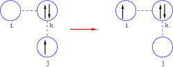
Figure 27: (Color online) Example for processes comprised in $\hat{H}_{V^{\prime}_{n}}$

Due to the constraint that site $k$ has to be occupied by a DO and site $i$ has to be empty in the beginning, these processes rely on the presence of two DOs which justifies to view them as true interactions. The number of DOs is not changed by this process. Processes such as $\hat{H}_{V^{\prime}_{n}}$ appear in second order of $\frac{t}{U}$.

The corresponding coupling constant is shown in the left panel of Fig. 28 as function of $W/U$. In the right panel of Fig. 28, the value for the coupling constant $V^{\prime}_{n}$ in the doped case is shown relative to its value in the half-filled case.

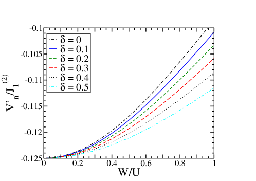
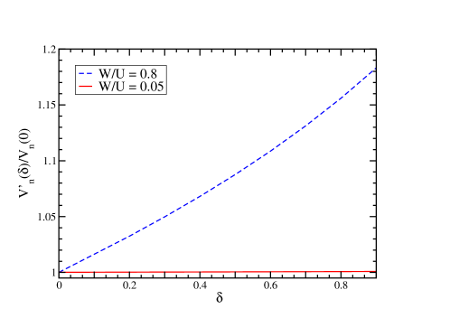
Figure 28: (Color online) Effective correlated hopping process $V^{\prime}_{n}$ over diagonal neighbors for various $\delta$ (left panel) and as function of $\delta$ for the values $W/U=0.05$ and $W/U=0.8$ (right panel). The undoped values are $V^{\prime}_{n}\approx-1.9518\cdot 10^{-5}\,U$ ($W/U=0.05$) and $V^{\prime}_{n}\approx-4.2584\cdot 10^{-3}\,U$ ($W/U=0.8$).

For large values of $W/U$, the coupling $V^{\prime}_{n}$ shows a noticeable dependence on $\delta$. Note that besides the correlated hopping defined in (42) and illustrated in Fig. 27, there is correlated hopping between three sites located on three sites in a row. The corresponding coupling constant $V^{\prime\prime}_{n}$ shows the same behavior as $V^{\prime}_{n}$ so that we do not show it here for brevity.

For too large values of $W/U$, i.e., $W/U\gg 1$, the curves for the coupling constants are not smooth anymore (not shown here) Reischl et al. (2004). This observation is explained by the breakdown of the mapping as it is indicated by the behavior of the apparent charge gap (see Sect. VI).

VII.4 Hopping Terms

The first term to be considered is $\hat{T}_{0}$ which was introduced before in (7a). The initial $\hat{T}_{0}$ represents hopping processes by one lattice spacing without a change in the number of DOs. The corresponding coupling constant $t_{0}$ is shown in the left panel of Fig. 29 relative to its unrenormalized value.

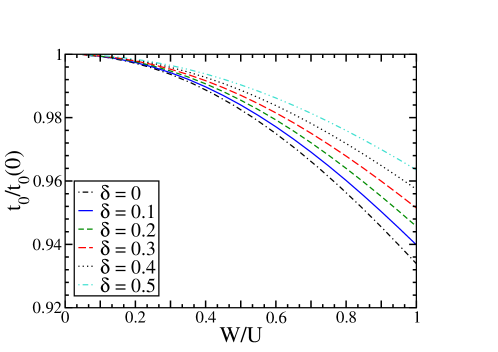
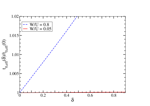
Figure 29: (Color online) Effective NN hopping without changing the number of DOs compared to its initial, bare value (left panel). Its doping dependence relative to the values at half-filling $t_{0}(0)\approx 6.2490\cdot 10^{-3}\,U$ for $W/U=0.05$ and $t_{0}(0)\approx 0.0956\,U$ for $W/U=0.8$ is depicted in the right panel.

The deviation of the coupling $t_{0}$ from its bare value is proportional to $\left(\frac{t}{U}\right)^{2}$. It is increased upon increased doping. To examine the doping dependence the renormalized value of $t_{0}$ in the doped case is compared to the one in the half-filled case in the right panel of Fig. 29. Under the influence of doping the hopping parameter is increased linearly. But even for $W/U=0.8$ the parameter is changed only by a few percent.

Hopping also occurs between diagonal sites on a plaquette, for instance in

$$\hat{T}^{\prime}_{0}=t^{\prime}\sum_{\sigma}\sum_{<<i,j>>}\left[\left(1-\hat{n}_{i,\sigma}^{\phantom{\dagger}}\right)\hat{c}_{i,\bar{\sigma}}^{\dagger}\hat{c}_{j,\bar{\sigma}}^{\phantom{\dagger}}(1-\hat{n}_{j,\sigma}^{\phantom{\dagger}})+\right.$$

$$\left.\hat{n}_{i,\sigma}^{\phantom{\dagger}}\hat{c}_{i,\bar{\sigma}}^{\dagger}\hat{c}_{j,\bar{\sigma}}^{\phantom{\dagger}}\hat{n}_{j,\sigma}^{\phantom{\dagger}}+\text{h.c.}\right]\,.$$ (43)

Here the double bracket under the sum indicates next-nearest neighbors (NNN) on the square lattice. The same process also appears between third nearest neighbors with a distance of two lattice sites. The corresponding coupling constant is denoted by $t^{\prime\prime}$. Since $t^{\prime\prime}$ and $t^{\prime}$ show very similar behavior we only show the results for $t^{\prime}$ in Fig. 30.

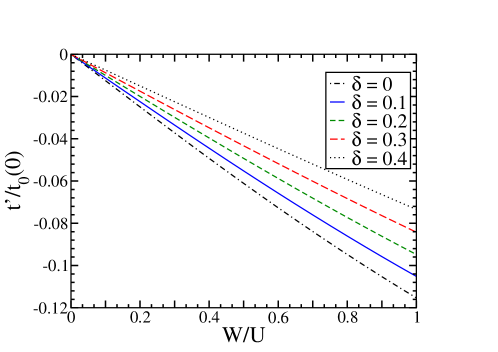
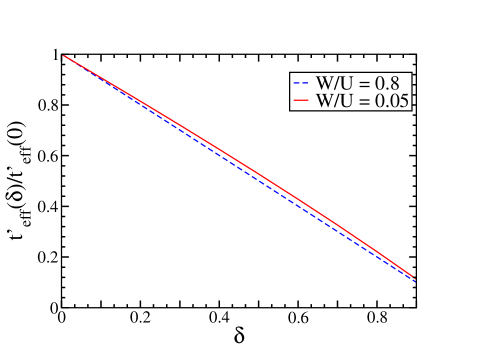
Figure 30: (Color online) Effective NNN Hopping $t^{\prime}$ between diagonal sites as function of $W/U$ for various values of $\delta$ (left panel) and its doping dependence for $W/U=0.05$ and $W/U=0.8$ (right panel). In the undoped case $t^{\prime}$ takes the values $t^{\prime}(0)\approx-3.9053\cdot 10^{-5}\,U$ ($W/U=0.05$) and $t^{\prime}(0)\approx-9.4785\cdot 10^{-3}\,U$ for $W/U=0.8$.

The hopping $t^{\prime}$ decreases linearly for increasing ratio $W/U$ with slopes depending on the doping, see left panel of Fig. 30. Relative to its values at half-filling the decrease as function of doping hardly depends on $W/U$, see right panel of Fig. 30. It is remarkable that the constant is decreased to almost 0 for $\delta\rightarrow 1$. This is actually the only significant dependence on doping that we found. But one has to keep in mind that the absolute values of $t^{\prime}$ are small. Note that the sign of $t_{0}$ is positive whereas $t^{\prime}$ and $t^{\prime\prime}$ are negative.

An interesting coupling generated in second order of $\frac{t}{U}$ is the spin dependent hopping described by

$$\hat{T}^{\prime}_{\text{spin}} =t^{\prime}_{\text{spin}}\sum_{\alpha\beta}\sum_{<i,k,j>}\left[\left[\left(1-\hat{n}_{i,\alpha}^{\phantom{\dagger}}\right)\hat{c}_{i,\bar{\alpha}}^{\dagger}\vec{\sigma}_{\bar{\alpha},\bar{\beta}}\hat{c}_{j,\bar{\beta}}^{\phantom{\dagger}}(1-\hat{n}_{j,\beta}^{\phantom{\dagger}})\right.\right.$$

$$\left.\left.+\hat{n}_{i,\alpha}^{\phantom{\dagger}}\hat{c}_{i,\bar{\alpha}}^{\dagger}\vec{\sigma}_{\bar{\alpha}\bar{\beta}}\hat{c}_{j,\bar{\beta}}^{\phantom{\dagger}}\hat{n}_{j,\beta}^{\phantom{\dagger}}+\text{h.c.}\right]\vec{S}_{k}\right]\hskip 28.45274pt$$ (44)

where the sum runs over two diagonal neighbors $i$ and $j$ which have a common nearest neighbor $k$. The size of the corresponding hopping parameter $t^{\prime}_{\text{spin}}$, see Fig. 31, is comparable to the spin independent parameter $t^{\prime}$. This shows that the induced NNN spin dependent hopping processes are as important as the spin independent ones. This was first observed by Reischl et al. Reischl et al. (2004) at half-filling.

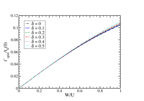
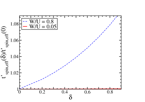
Figure 31: (Color online) Effective spin dependent hopping $t^{\prime}_{\text{spin}}$ for various values of $\delta$ (left panel) and its dependence on $\delta$ for two values of $W/U$, namely $W/U=0.05$ ($t^{\prime}_{\text{spin}}(0)\approx 3.9042\cdot 10^{-5}\,U$) and $W/U=0.8$ ($t^{\prime}_{\text{spin}}(0)\approx 8.8496\cdot 10^{-3}\,U$) (right panel).

Upon doping the spin dependent hopping term is increased. But even for larger values of $W/U$ the value of $t^{\prime}_{\text{spin}}$ is increased only by a few percent. The analogous process also appears between third nearest neighbors. The corresponding coupling constant behaves similar to $t^{\prime}_{\text{spin}}$ so that we do not display it here. Both processes concern three sites. Thus it does not matter significantly whether the sites are aligned linearly or in a right angle on a plaquette.

Compared to the spin independent hopping $t^{\prime}$ the spin dependent hoppings $t^{\prime}_{\text{spin}}$ and $t^{\prime\prime}_{\text{spin}}$ are not negligible. But all of them are fairly small compared to the bare NN hoping $t_{0}$. Thus one can either stick to a pure $t$-$J$ model or include more extended hopping terms. But if one opts for including hopping over two lattice spacings one should incorporate spin independent hopping $t^{\prime}$ as well as the spin dependent hoppings $t^{\prime}_{\text{spin}}$ and $t^{\prime\prime}_{\text{spin}}$. The doping dependence of the spin dependent hopping elements may be neglected. In contrast, the hopping element $t^{\prime}$ shows a rather strong dependence on the doping concentration $\delta$.

VIII Summary

We presented a systematically controlled mapping of a fermionic Hubbard model to a generalized $t$-$J$ model. The conceptual foundation of this mapping was analyzed carefully. In particular, we developed a scheme for this mapping which covers also the interesting case of substantial doping. Remarkably, this issue had so far attracted only little attention.

In the derivation of the generalized $t$-$J$ model we eliminate the charge fluctuations by self-similar continuous unitary transformations. Processes that change the number of double occupancies are rotated away. Thereby, we obtain the effective coupling constants as function of the doping $\delta$ and of the ratio $W/U$ where $W$ is the bandwidth and $U$ the local interaction. Note that the generalized $t$-$J$ model comprises the magnetic degrees of freedom as well as the kinetics and the interactions of double occupancies.

We extended the concept of the apparent charge gap $\Delta_{g}$ Reischl et al. (2004) from half-filling to the doped system. This gap is not the true physical gap but it measures the energy separation of subspaces with differing number of double occupancies irrespective of the spin state. We argue that as long as $\Delta_{g}$ is finite the mapping to a $t$-$J$ model is justified. A vanishing $\Delta_{g}$ indicates the breakdown of this mapping. By estimating the parameter where $\Delta_{g}(W/U,\delta)=0$ holds we derived a diagram of applicability of the $t$-$J$ model shown in Fig. 15. As expected the applicability is reduced upon doping $\delta$. But it levels at intermediate values of doping so that the commonly assumed parameters for the description of high-$T_{c}$ cuprates lie within the range of applicability. To our knowledge, no such result was derived before.

Furthermore we find that the coupling constants of the effective model show hardly any doping dependence. The only coupling which exhibits a significant dependence on $\delta$ is the hopping parameter $t^{\prime}$ describing hopping between diagonal neighbors. Relative to its value at half-filling $t^{\prime}$ exhibits a strong doping dependence. But the absolute value of this hopping element remains small. Thus within a wide range of doping the $t$-$J$ model with constant coupling constants is appropriate. Besides the usually considered terms, the 4-spin ring exchange on each plaquette should be included.

Technically we used recently developed types of infinitesimal generators for the continuous unitary transformation Fischer et al. (2010). They only decouple certain subspaces of the Hilbert space which simplifies and accelerates the calculations. So far, the pc-generator was used which leads to a particle number conserving effective model; the particles are the double occupancies Reischl et al. (2004); H.-Y.Yang et al. (2010). We extended the gs-generator introduced previously for the ground state of matrices Dawson et al. (2008) and of many-body systems Fischer et al. (2010) to mixed reference ensembles. The gs-generator is particularly suited to obtain the purely magnetic Heisenberg model since it efficiently decouples the subspace of the reference ensemble from the remainder of the Hilbert space. If, however, the dynamics of the double occupancies matters as well, the gs,1p-generator turned out to be a good compromise between efficiency and sufficient decoupling. This generator decouples the reference ensemble and the states with one double occupancy from the rest of the Hilbert space. We found that the couplings derived from a faster gs,1p-calculation agree very well with the results from a slower pc-calculation. We expect that these generator or modifications of them will continue to play an important role in the systematic derivation of effective models.

The present analysis for the square lattice can certainly be extended to other types of lattices such as the triangular lattice which has already been analysed by perturbative CUTs H.-Y.Yang et al. (2010), the honeycomb lattice Meng et al. (2010), or more sophisticated lattices such as the kagomé lattice and so on. In this way, the effects of subleading magnetic exchange processes such as ring exchange can be analysed quantitatively.

Another route to extend the present calculation is to also transform the observables, for instance the standard fermionic creation operator. At half-filling, one will then be able to compute the spectral weight in the upper Hubbard band, that means in the subspace with one double occupancy. But there should be also weight in the subspaces with three and more double occupancies. To our knowledge, no estimate whatsoever exists for the weight in such trans-Hubbard bands.

More generally, the systematic derivation of effective models in other contexts can be tackled by adapting the ideas of the present work. For instance, the reliable downfolding of interacting fermionic models with many bands to models with a minimum number of bands and Hubbard-type of interactions is a long standing field of research Herbst et al. (1978a, b); Gunnarsson (1990) which continues to attract much attention, see for instance Refs. Aryasetiawan et al., 2004; Cano-Cortés et al., 2007; Miyake and Aryasetiawan, 2008; Cano-Cortés et al., 2010. We think that continuous unitary transformations provide an promising approch to make systematic and controlled progress in this field.

Hence we expect that the systematic derivation of effective models by means of continuous unitary transformations will continue to evolve into a field with widespread applications.