Characterisation of Sloan Digital Sky Survey Stellar Photometry

Abstract

We study the photometric properties of stars in the data archive of the Sloan Digital Sky Survey (SDSS), the prime aim being to understand the photometric calibration over the entire data set. It is confirmed that the photometric calibration for point sources has been made overall tightly against the SDSS standard stars. We have also confirmed that photometric synthesis of the SDSS spectrophotometric data gives broad band fluxes that agree with broad band photometry with errors no more than 0.04 mag and little tilt along the wide range of colours, verifying that the response functions of the SDSS 2.5 m telescope system are well characterised. We locate stars in the SDSS photometric system, so that stars can roughly be classified into spectral classes from the colour information. We show how metallicity and surface gravity affect colours, and that stars contained in the SDSS general catalogue, plotted in colour space, show the distribution that matches well with what is anticipated from the variations of metallicity and surface gravity. The colour-colour plots are perfectly consistent among the three samples, stars in the SDSS general catalogue, SDSS standard stars and spectrophotometric stars of Gunn & Stryker, especially when some considerations are taken into account of the differences (primarily metallicity) of the samples. We show that the $g-r$ - inverse temperature relation is tight and can be used as a good estimator of the effective temperature of stars over a fairly wide range of effective temperatures. We also confirm that the colours of G2V stars in the SDSS photometric system match well with the Sun.

1 Introduction

The Sloan Digital Sky Survey (York et al., 2000, SDSS) provides a large data base of photometry for galaxies and stars, over 350 million objects in the 11663 square degree survey area, that can be used for a great variety of astrophysical science (Abazajian et al., 2009). Besides its scale, another very important feature is the special care that has been paid to maintain the accuracy of the data, especially their photometric accuracy, from instrumentation throughout the eight year period of the survey. The photometric system is different from systems which have been traditionally used, so it must be internally defined consistently over that period. In addition, the survey attempted to apply photometric calibration to the over 1 million spectra obtained during the survey, and we will study this calibration as well.

One of the important issues is the consistency between spectrophotometry and broad-band photometry with the five passbands, in the sense that the integral of spectrophotometric data with the determined response functions should give the proper broad-band flux. This has been a perennial problem inherent with the data bases available to date. Synthetic colours obtained by integrating spectrophotometric data often give systematically increasing error with colours as obtained by broad band photometry, typically of the order of 0.1 mag, or sometimes larger, for stars for a range in $B-V$ from 0 to 1 (see e.g., Fukugita, Shimasaku & Ichikawa, 1995). This is probably largely to be attributed to a poor characterisation of the response functions of conventional detector systems.

In order to minimise these systematic errors and make the broad-band photometry as well specified as possible, much effort was invested in the SDSS to characterise the response functions (Doi et al., 2010), in addition to a chain of stellar calibrations (Tucker et al., 2006; Stoughton et al., 2002). The response functions for SDSS photometry have been measured on site a number of times during the survey, which enables us to characterise their seasonal and secular variations. This work has been published in Doi et al. (2010), where the representative response functions are also presented as the Reference response functions of the 2.5m telescope (Gunn et al., 1998, 2006). These average response functions are recommended to be used unless the user’s interests are in fine details. It is demonstrated in Doi et al. (2010) that the stellar data taken in the early period of the survey are consistent with those acquired in the later period within 0.01 mag after calibration, including the data for the $u$ passband which has suffered from a significant secular change in the system response and, therefore, the expected variations in photometry have been well compensated by the calibration process. It is concluded that the errors due to time varying changes, both seasonal and secular, in the response functions and calibration procedures that use several different systems are no more than 0.01 mag as a whole.

The other special feature of the SDSS observation is hourly monitoring of the atmospheric extinction with the ancillary 50-cm Photometric Telescope (PT). A set of the SDSS standard stars were observed every night, together with hourly observation of stars in the transfer fields from PT to the 2.5-m main telescope. The SDSS standard stars are chosen as uniformly as possible both over the northern sky and in colour space so that they are not inclined to give weight towards particular classes of stars (Smith et al., 2002). For other efforts to maintain the accuracy of the photometry, see Hogg et al. (2001); Tucker et al. (2006); Ivezić et al. (2004).

In this paper we study the photometric accuracies and properties of the data presented in the SDSS catalogues, which are already in the public domain. The purpose of this paper is to examine, in particular, (i) the consistency between spectrophotometry and broad-band photometry, including the verification of the response functions for broad band photometry, (ii) the overall accuracy of photometric calibrations against standard stars, (iii) the location of stars in colour space in the SDSS photometric system and its variation with the atmospheric parameters of stars, such as effective temperature, surface gravity and metallicity, (iv) colours of galaxies relative to stars, and (v) brightness and colour of the Sun in the SDSS photometric system. One of the important purposes of (iii) is to locate stars of known spectral type in colour space so that approximate spectral type can be inferred from colours of the SDSS photometric system. We also give effective temperature for those stars. The reader is referred to Lenz et al. (1998) for an earlier study along these lines. There is also a substantial amount of work done for observations of stars and for determinations of the atmospheric parameters in Sloan Extension for Galactic Understanding and Exploration (SEGUE) under the SDSS project (see, Lee et al. (2008a, b); Allende Prieto et al. (2008); Yanny et al. (2009)). Here, the problem is that the SDSS acquired spectra of stars fainter than $g\simeq 14$, whereas the stars for which high resolution spectra are available needed to determine the atmospheric parameters are brighter, such as $V<14$ (NB: $V\approx g-0.1$): hence, the overlap of the samples is small, which makes well-calibrated stellar science with the SDSS not so straightforward. This also remains as our problem and we attempt to circumvent it by the use of bright SDSS standard stars, or of spectrophotometric standard stars after verifying their brightness in the SDSS photometric system.

The procedure of SDSS broad band photometry is described in Tucker et al. (2006); see also Stoughton et al. (2002). In brief it is based on the network of 158 standard stars spanning a wide range of colours, which were measured by separate observations made at USNO (Smith et al., 2002) using filters and a detector system pseudo-equivalent to the SDSS system (Doi et al., 2010) with the colour tansformation between the two systems taken into account to offset the slight difference in their response functions. The zero point is ultimately set by the subdwarf BD$+17\arcdeg 4708$ whose brightness is defined by a synthetic calculation of the spectrophotometric data (Oke & Gunn, 1983; Oke, 1990) in the AB₉₅ magnitude system (Fukugita et al., 1996). The main telescope data are calibrated using the set of stars which are observed simultaneously with both the main telescope and an ancillary 50 cm Photometric Telescope, the latter being also used to observe the SDSS standard stars whose brightness is set by the work at USNO, and to monitor hourly atmospheric extinction during survey operation.

Spectroscopy was carried out with two fibre-fed double spectrographs covering the wavelength range 3800 to 9200Å  with two 2048²-pixel CCD detectors in each spectrograph. The spectrographs are fed with 640 fibers plugged into an aluminum plate in the focal surface, positioned with the astrometry obtained from the imaging data (Pier et al., 2003). The mean resolving power is $\Delta\lambda/\lambda\simeq 1850-2200$ depending on the wavelength. Spectrophotometric calibration is carried out using spectrophotometric standard stars selected in each field. Standard stars were intended to be typically F8 dwarfs (Abazajian et al., 2004) but the set in actuality contains a variety of similar spectral types (Adelman-McCarthy et al., 2008); the spectra are fit to models given by Gray et al (2001), and the model spectra are used for calibration. Spectrophotometric calibration also requires match between spectrophotometric fluxes and the broad-band photometric PSF fluxes. This is done with a single calibration determined for each camera in a given plate (Adelman-McCarthy et al., 2008).

The data acquired in the SDSS projects are all published in 7 data releases, DR1$-$DR7 (Abazajian et al., 2003, 2004, 2005; Adelman-McCarthy et al., 2006, 2007, 2008; Abazajian et al., 2009). All DR data are cumulative, and DR7 stands for the final data release of the SDSS I and II, which employ the original instrumentation of the SDSS. We use the data set from DR6 in the study presented in this paper. The photometric calibration is made against the set of standard stars. Reddening corrections are not applied for the stars. The stars are located mostly in low extinction regions. If we take the extinction map of Schlegel et al. (1998), the peak of the distribution is at $(B-V)\approx 0.02$ with the mean 0.04 and the variance 0.03; only 2.6% of stars are located in the region $E(B-V)>0.1$. Note that this reddening is the maximum value along the line of sight and the actual reddening for objects within the disk of the galaxy is smaller.

2 Comparison between spectrophotometry and broad-band photometry

In this paper we consider synthetic fluxes, obtained by integrating with the $d\ln\nu$ measure over the spectrophotometric data with the response functions for each filter. The flux calibration of the spectrophotometry was done by comparing the spectrophotometric data with the PSF fluxes of the standard stars in each spectroscopic field (actually two fields independently, one for each spectrograph.) So, it is important to confirm that synthetic spectrophotometric fluxes indeed agree with broad band photometric fluxes within tolerable errors for the majority of stars across the wide spectral range.

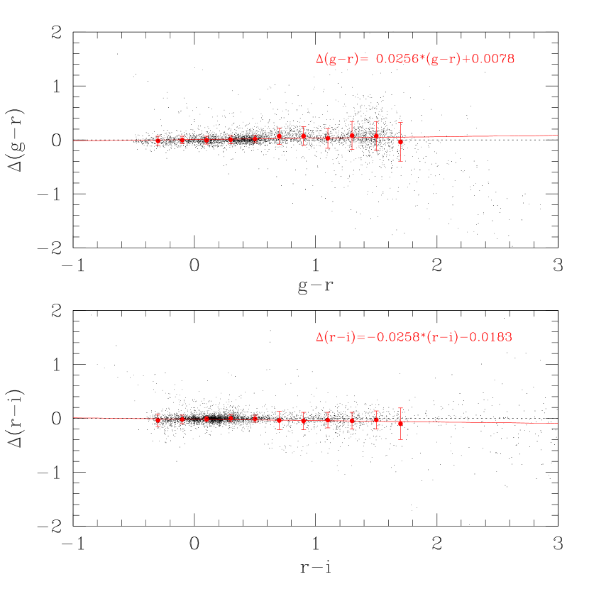
Figure 1: Difference in the brightness of broad band colour between the synthesis of the spectrophotometric data and the direct broad band photometry, $m({\rm spectro})-m({\rm photo})$, is plotted against colours of stars acquired in the southern equatorial stripe (Stripe 82) for $g-r$ and $r-i$. The lines are linear fits with the coefficients given in the figure.

In Figure 1 we present the difference of synthetic colours and photometric colours for (a) $g-r$ and (b) $r-i$ as a function of colours of stars. Stars are taken from the observation for southern equatorial stripe (stripe 82), and the psf magnitude is adopted for broad band photometry. The error bar shows the variance in each colour bin, 0.2 mag in $g-r$ or $r-i$. The offset of the mean is $<0.05-0.07$ mag for most of the colour bins, and it increases to 0.08 mag for red stars with $g-r\approx 1.3$. The rms scatter we have seen is about 0.1 mag, and it goes up to $>0.15$ mag towards redder stars with $g-r>0.7$. This is compared with the rms error quoted for the spectrophotometric calibration, 0.04 mag (DR7). The smaller scatter for bluer stars offsets the larger rms scatter in longer wavelengths for the total sample.

The $u$ and $z$ passbands are out of the range of our spectroscopy, which spans from 3800Å to 9200Å  and therefore are not shown. We adopt the SDSS spectroscopic data and use the reference response function for the SDSS 2.5 m telescope presented in Doi et al. (2010) referred to the standard 1.3 airmass value for the atmospheric extinction corrections.

The global tilt of the offset across colour is small. After 3$\sigma$ rejection of highly deviant data points, the mean gives $\Delta(g-r)_{\rm spec-photo}=0.026(g-r)+0.008$ and $\Delta(r-i)_{\rm spec-photo}=0.026(r-i)-0.018$ for the range $-0.4<g-r<1.8$ and $-0.4<r-i<1.8$, respectively. This implies that the response curves are well characterised. Synthetic colours may be substituted for broad band measurements at least in the mean over the stars in the sample and for non-variable stars. We consider that this is an improvement, crudely speaking, of a factor of 5 in accuracy compared with previous ‘best’ spectrophotometry-photometry data sets (e.g., Fukugita et al., 1996). Highly deviant data points are likely to be variable stars or double stars, as found for subsamples (Sesar et al., 2007).

3 Colours of stars in the SDSS data base

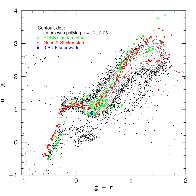
Figure 2: Three hundred thousand stars in $u-g$ vs $g-r$ colour space taken from SDSS general star catalogue. Densely populated regions are shown by contours, and one step corresponds to $\sqrt{10}$ increase in the density with the outermost contour for 75 stars/(0.1 mag)². Open circles show SDSS standard stars, and solid circles are the GS83 stars. Those denoted by solid squares are three BD F-subdwarfs, taken to give the observational flux standard. The oblique line segment along the contour (from $g-r=0.2$ to 0.8) indicates the approximate positions of the centre of gravity for the star distribution used to define $d_{ug}$ used in later figures.

In Figure 2 we plot $u-g$ of 290647 stars with $16.95<r<17.05$ against $g-r$ taken from the full DR6 catalogue. Regions of densely populated points are represented by contours, which correspond to an increase of density by $\sqrt{10}$ in each step. Those denoted by individual points are 2660 stars, or 0.9% of all stars. The catalogue contains an additional 583 stars that fall outside the range and are not plotted. We also superimpose the data of 158 SDSS standard stars given in Smith et al. (2002) and 175 spectrophotometric stars given by Gunn & Stryker (1983, hereafter GS83). The colour of GS83 stars is derived by synthetic calculations with the reference response function of the 2.5m telescope system at 1.3 airmass after taking the redleak of the $u$-filter into account. Since the GS stars are mostly located in the low latitude field and receive large reddening, dereddening correction is applied as in GS93. It is noted that the reddening model used in that paper is probably oversimple, although the resulting colour does not differ too significantly from what is calculated using a more standard extinction curve.

There are 5 GS83 stars that fall beyond the figure frames and are dropped. All SDSS standard stars are shown. The redleak affects $u-g$ colour by no more than 0.02 mag for stars with $g-r\leq 1$, while it increases to 0.2 mag close to the red edge of the contour, $g-r\approx 1.5$. Recognition of this correction improves agreement between the GS83 stars and other stars, if only slightly. The three solid squares around $g-r\approx 0.28$ represent the metal poor F subdwarfs, BD$+17\arcdeg 4708$, BD$+26\arcdeg 2606$ and BD$+21\arcdeg 0607$, the latter two of which were added to the first to set up the network of F-subdwarf standards approximately 8 hours apart (Smith et al., 2002). Accurate spectrophotometry is available only for the first two stars (Oke & Gunn, 1983; Oke, 1990), but the third is sufficiently similar to the first two that the adopted linear interpolation to obtain its fluxes should be adequate.

We confirmed that the contours of the distribution of stars change only moderately when we take stars of $r\simeq 18$ or 19 instead of $r\simeq 17$. The distributions change in detail, doubtless due to the changes in stellar populations from old disk to thick disk and halo as one goes fainter (Chen et al., 2001; Ivezić et al., 2008). The contours, however, overlap very well for stars bluer than $g-r\simeq 1$ for the 3 samples that differ in brightness, indicating that the calibration is robust against brightness of stars.

We see that both SDSS standard stars and GS93 stars are located near the centre of gravity of the distribution of stars in the SDSS general sample for $g-r<0.8$. This also serves, albeit indirectly, as the evidence that spectrophotometry of the GS83 stars and spectroscopic synthesis give correct broad band colours to the level we have required. We see for red stars with $g-r>0.7$ some shift of the loci of these stars towards the upper side, $u-g$ being redder by $\approx 0.3$ mag. On the other hand there appears a second locus of the GS83 stars, which is shifted downwards by $\approx 0.1$ mag with respect to the centre of gravity. We ascribe this to widening of the gap in colour space between the distribution of luminosity class III and V stars for $g-r\geq 1$, as shown in the next section. For red stars we observe that the locus of the GS83 stars is more heavily populated around the upper side, to which stars are driven by high metallicity (nearly solar) of the GS83 stars. In general, the scatter becomes larger towards the redder end, as a natural wilder variation of spectra due to molecular bands developed in later K to M stars for $g-r\geq 1$. The span of the $u-g$ colour range against the variation of metallicity, and also of gravity, increases towards the reddest stars.

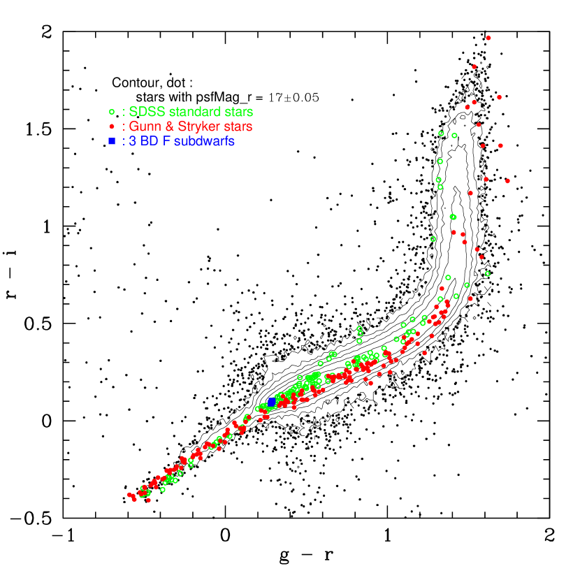
Figure 5: Same as Figure 2, but for $r-i$ vs. $g-r$.

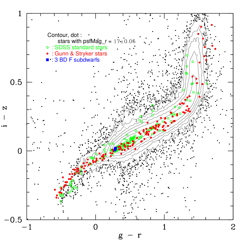
Figure 6: Same as Figure 2, but for $i-z$ vs. $g-r$.

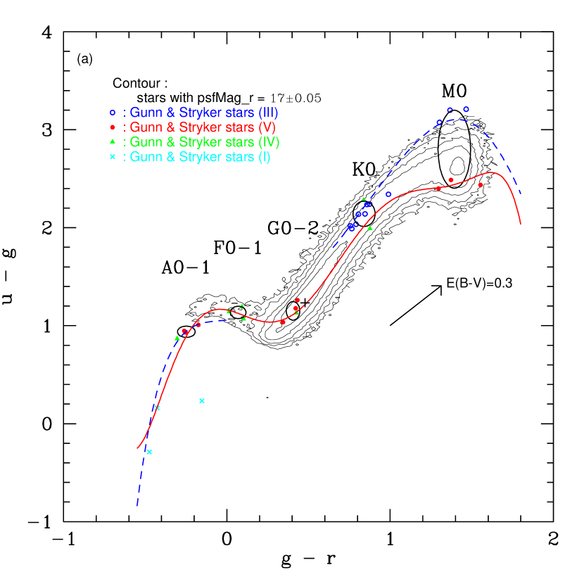
Figure 8: (a) Distribution of stars in the SDSS general catalogue in $u-g$ vs. $g-r$ plane (the same as Figure 2 but with isolated points representing individual stars suppressed). Two curves are empirical loci of main sequence stars obtained by interpolating the GS83 stars with known spectroscopic types separately for luminosity class V (solid curve, red) and III (dashed curve, blue). In panel (a) ellipses show the position of the GS83 stars with types given as indicated in the figure with the size representing the variance of the subsample. The plus symbol is colour of the Sun given in the text. In panel (b) [ see next page ] line segments indicate variations due to metallicity from [Fe/H]=$-1$ to +1 with 0.5 unit steps (blobs), from downstairs up, using the Kurucz atmosphere model. Asterisks show the position for [Fe/H]=$0$.

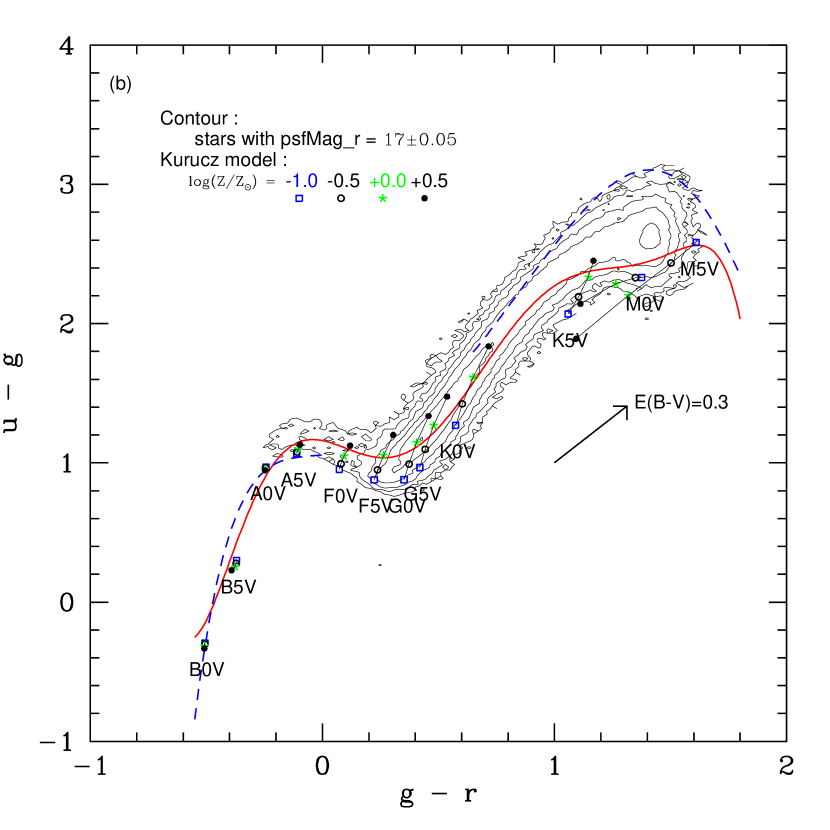
Figure 8: (b) continued

For very blue stars with $g-r<-0.2$, the locus of the GS83 stars does not agree with that of SDSS standard stars and that of the general SDSS stars, by 0.1 mag in $g-r$ or as much as 0.4 mag in $u-g$. This is significantly larger than could arise from the different response functions of SDSS specifications. One might suspect that this displacement is due to reddening, especially given the crudity of the GS reddening corrections. In fact, however, the displacement corresponds approximately to $E(B-V)\approx 0.15$. Such large extinction is very rare in the SDSS data, but is present in essentially all the blue GS stars, and is poorly determined. However, if such corrections are systematic and are made, we would expect shifts in $i-z$ vs $g-r$, for which the shift (see Figure 6 below), if any, takes place in a way opposite to that expected. Note that the standard extinction curve (O’Donnell, 1994) gives reddening for $r-i$ and $i-z$ smaller than that for $u-g$ only by a factor of two (see arrows for extinction in Figure 8-12 below). In $r-i$ vs $g-r$ the two loci overlap at a good precision; see Figure 5 below, but the extinction for this colour is nearly parallel to the stellar locus, and it is not easy to separate out extinction. We thus do not find an easy explanation that accounts for the shift in $u-g$ vs $g-r$ plane between the GS83 stars relative to the SDSS stars. We do note, however, that the populations of the blue GS stars and the blue SDSS stars are completely different; the blue GS stars are all main-sequence disk Population I objects, and the blue SDSS stars are essentially all low-mass, hot, highly evolved Population II objects of a variety of types, so the discrepancy may not be surprising. We note also that the locus of the SDSS stars overlaps well that of the SDSS standard stars.

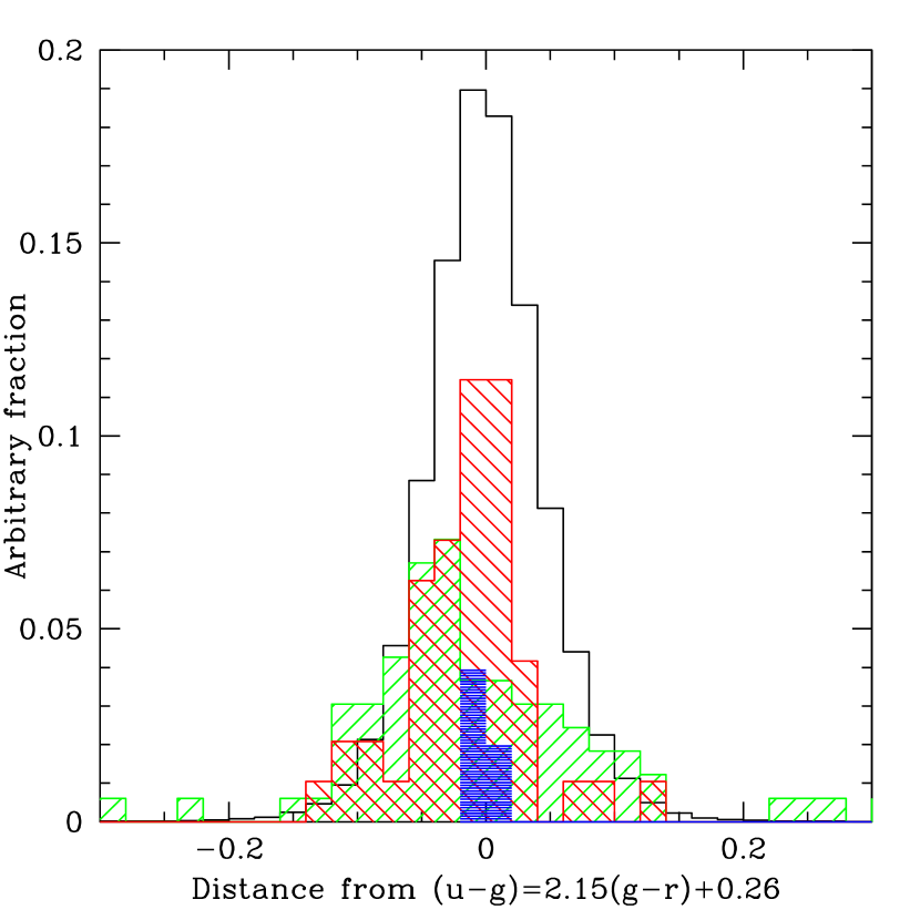
Figure 3: Distribution of stars with $0.2<g-r<0.8$ in different samples projected to the axis that is perpendicular to the distribution of densely populated region, which is around $u-g=2.15(g-r)+0.26$ in $g-r$ vs $u-g$ colour space, shown in Figure 2. The abscissa is $d_{ug}$ (mag). Open histogram shows the stars in the general SDSS catalogue, the histogram hatched from up-left to down-right (red) shows stars in the GS83 sample, and that hatched from up-right to down-left (green) shows the SDSS standard stars presented in Smith et al. (2002). The thick horizontally hatched histogram at around the zero point in the abscissa shows 3 F subdwarfs taken as the fundamental standard at the observation. The ordinate is in arbitrary units.

To scrutinize the possible offset among the populations in three different star samples, i.e., the sample in the SDSS general catalogue, the SDSS standard star sample and the GS83 sample, we plot in Figure 3 the distribution of the three populations, projected onto the line orthogonal to $(u-g)=2.15(g-r)+0.26$ which follows the locus of the stellar colour for $0.2\leq g-r\leq 0.8$, indicated as the line segment in Figure 2. The distribution of the three F subdwarfs is also shown. The distance along this base line measured from the locus of the population is denoted by $d_{ug}$ (mag) with the positive direction towards the lower right (increasing $g-r$ and decreasing $u-g$). We see that all populations are distributed very well with respect to the common zero point, although the distribution for the SDSS standard stars is somewhat skewed towards the bluer side, which can be understood by a larger weight of lower metallicity stars in that sample. No alarming offset is visible in the zero point among the four samples beyond $\approx 0.05$ mag in $d_{ug}$.

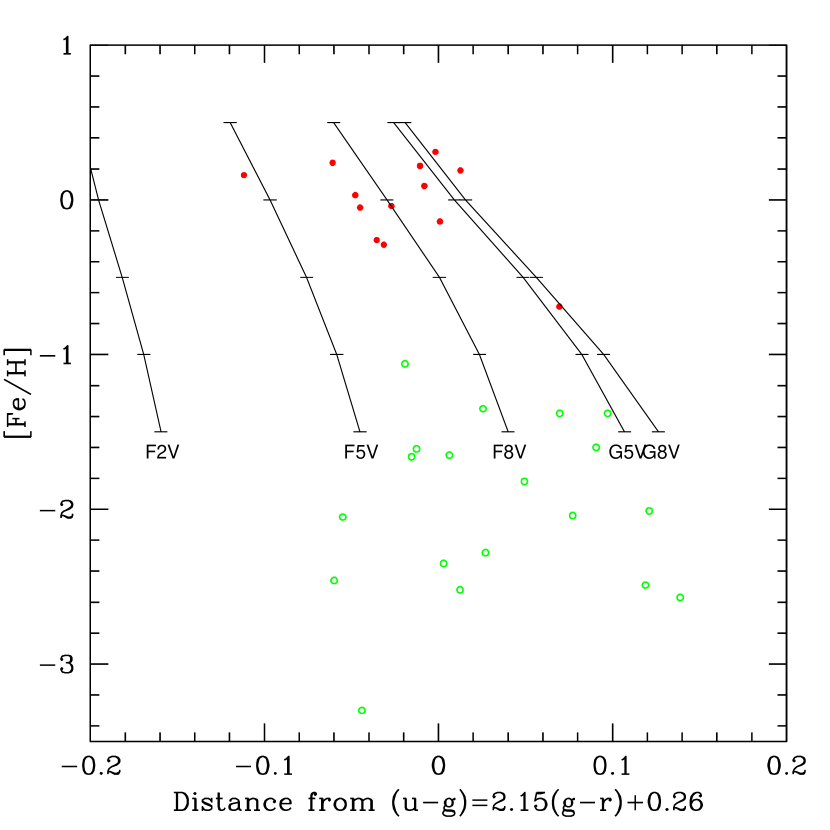
Figure 4: Correlation of [Fe/H] estimated in Cayrel de Strobel et al. (2001) with $d_{ug}$, i.e., the distance from the line $(u-g)=2.15(g-r)+0.26$, which represents the centre of gravity of the most densely populated region between $g-r=0.2$ and 0.8, as defined in the text. The sample is taken from the GS83 stars (solid circles) and the SDSS standard stars (open circles). The line segments are the metallicity dependence predicted by the Kurucz atmosphere model (Castelli & Kurucz, 2004) from F2 to G9 stars in the main sequence.

The distance $d_{ug}$ is correlated with metallicity. 21 out of the 158 SDSS standard stars and 44 out of the 175 GS83 stars are given estimates for metallicity with high resolution spectroscopic observations (Cayrel de Strobel et al., 2001). Figure 4 shows those stars having colours in the range $0.2<g-r<0.8$ plotted in the plane of metallicity versus $d_{ug}$, indicating the correlation of metallicity with $d_{ug}$. It shows that the GS stars plotted in this figure have metallicity close to solar, while many of the SDSS standard stars are indeed metal poor [Fe/H]$<-1$, as expected from the fact that they are mostly high latitude halo objects (Ivezić et al., 2008). Although these are partial samples of the GS83 and the SDSS standard stars, this explains the difference of the two samples we saw in the $u-g$ vs. $g-r$ plane. We also plot the bundle of line segments which show the prediction of the Kurucz atmosphere model (Castelli & Kurucz, 2004) for stars with F2V to G8V, metallicity from [Fe/H]=0.5 being at the top to $-1.5$ at the bottom.

A similar plot is shown in Figure 5 for $r-i$ vs. $g-r$. The distribution is narrower and the agreement among the three distributions is much tighter than we have seen for $u-g$ vs. $g-r$. The SDSS standard stars are located very close to the centre of gravity of the general star sample. The GS83 stars are also located close to the centre of gravity: we observe a slight displacement between the SDSS standard star sample and the GS83 star sample, which is of the order of the difference we expect from the different metallicity. The three F subdwarfs are also on the top of the loci. The difference in the loci between the luminosity class III and V is negligibly small, as we see in the next section more quantitatively.

A similar observation holds for the plot of $i-z$ against $g-r$ shown in Figure 6. We do not observe displacements among the three populations, again except for some disagreement for very blue stars. Otherwise, the distributions of the standard stars and GS83 stars agree well with those of the stars in the SDSS general catalogue.

These considerations mean that the stellar loci are well defined in the SDSS photometry and depend little on the sample taken, and also verify that the photometric calibration has been made well in colour against the standard stars. This does not mean that the broad band flux is accurate in physical units (AB magnitude system), however.

4 Variations of colours and stellar atmosphere

The main parameters that regulate colours of stars are effective temperature $T_{\rm eff}$, surface gravity $g$ and metallicity [Fe/H]. We first show that $T_{\rm eff}$ is well represented by $g-r$ colour (see also Ivezić et al. (2008)). The most accurate measurement of $T_{\rm eff}$ is made with Michelson interferometry of stars to measure their diameters. This has been done, however, only for very bright stars and the sample is very limited. The sample may be extended by stars for which temperatures have been obtained from the infrared flux method (IRFM) (Blackwell & Shallis, 1977), which is calibrated against stars with Michelson interferometry measurements of high accuracy. The IRFM suffers from less model dependence; temperatures from the IRFM method are supposed to be accurate at the 1% level. The stars with effective temperatures estimated by IRFM are still too bright for the main sample of SDSS, but the GS83 sample has stars whose effective temperature has been estimated with IRFM. The argument in the previous sections ensures that photometry from spectrophotometric synthesis for GS83 stars is sufficiently accurate.

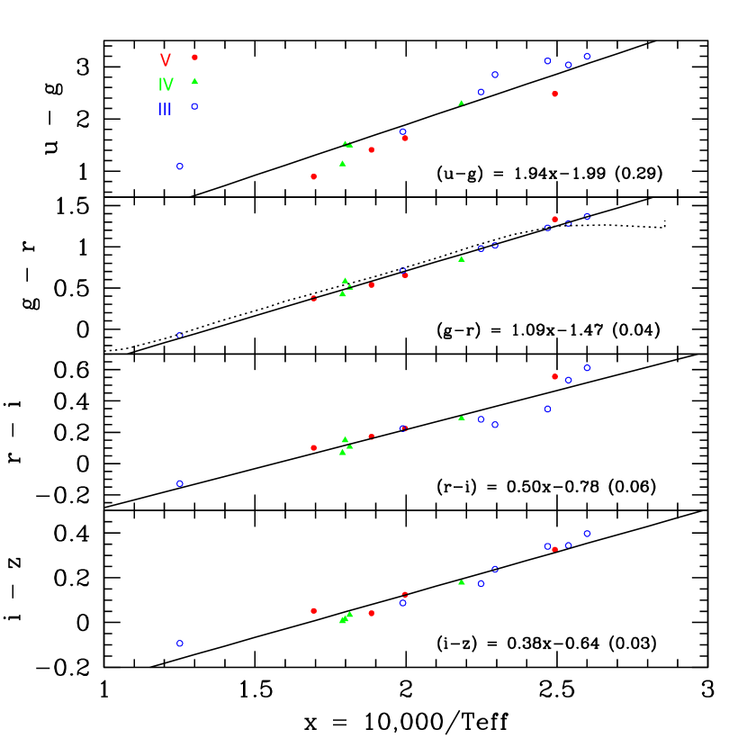
Figure 7: $u-g$, $g-r$, $r-i$ and $i-z$ colours plotted against inverse temperature in units of 10000K. The GS83 stars for which temperature is estimated using the IRFM are shown. The solid circles (red) show stars with the luminosity class V, open circles (blue) stars with luminosity class III and solid triangles (green) stars with luminosity class IV. Lines are linear fits to the data and their coefficients given in the figure where parentheses are dispersion of the fit in colour units. In the fit $x=10^{4}{\rm K}/T_{\rm eff}$ and $y$ is the corresponding colour. The dotted curve in the panel for $g-r$ is the prediction of the Castelli-Kurucz atmosphere model for main sequence stars.

Figure 7 shows colours of 15 GS83 stars against inverse effective temperature that is given in the IRFM catalogue of di Benedetto (1998). Among the panels that show $u-g$, $g-r$, $r-i$ and $i-z$ colours the correlation with $g-r$ colour is tightest: the stars are well fitted with the simple formula

$$T_{\rm eff}/10^{4}{\rm K}={1.09\over g-r+1.47}$$ (1)

with an rms scatter around the fit $\sigma_{g-r}=0.04$ or $\sigma(T_{\rm eff})=93$K. Note that the star sample contains different luminosity classes, III (7 stars), IV (4 stars) and V (4 stars), and metallicity is not differentiated. We do not observe any systematic difference for $g-r$ among the different luminosity classes. We note, however, that this colour-temperature relation is empirically verified only in the range, $1.25<10^{4}{\rm K}/T_{\rm eff}<2.6$ or $3850{\rm K}<T_{\rm eff}<8000{\rm K}$. The use of the Castelli-Kurucz atmosphere model (indicated by the dotted curve in the second panel of Figure 7) suggests that this inverse linear relation may break down for $T_{\rm eff}>9500{\rm K}$: for those stars with temperature higher than $T_{\rm eff}\approx 8500{\rm K}$, $T_{\rm eff}$ is higher than eq.(1) indicates for given $g-r$. A departure from eq.(1) is also indicated towards lower temperature below 3850K.

The expression we derived above agrees well with the $\log T_{\rm eff}-(g-r)$ colour relation given by Ivezić et al. (2008) but only in a finite segment, $-0.3<g-r<0.7$, or $5000<T_{\rm eff}<8000$K. The latter relation gives temperature significantly lower than the IRFM estimate for stars redder than $g-r\simeq 0.7$. Lee et al. (2008a) use a polynomial which is third order in $g-r$ to estimate $T_{\rm eff}$ from $g-r$ in the SEGUE stellar parameter pipeline. It agrees with eq. (1) within 0.02 dex for the range $-0.6<g-r<1.2$ ($4200K<T_{\rm eff}<12500$K).

We see some systematic shifts among different luminosity classes for the $u-g$ vs. inverse temperature plot; e.g., all 4 class V stars lie below the fit line, and 6 of the 7 class III stars lie above the line. The $i-z$ colour is also well correlated with temperature, the dispersion of $i-z$ being also small (0.03). The corresponding dispersion of temperature, $\sigma(T_{\rm eff})=190$K, however, is twice as large as that for the $g-r$ inverse temperature relation due to the shallower slope.

Metallicity has been estimated with high resolution spectroscopy (Cayrel de Strobel et al., 2001) for 9 among the 15 stars given in this figure and it ranges from [Fe/H]=$-$0.69 to 0.31. We do not observe a systematic trend with metallicity in the $g-r$ vs. $T_{\rm eff}$ plot. The variation with metallicity is significantly smaller than is seen with $B-V$, since the metal lines are fewer and weaker in the $g$ (and $r$) passband than in the $B$ passband. The scatter around the colour temperature relation is nearly as small as the one that would be obtained after the metallicity effect taken into account in the $B-V$ - $T_{\rm eff}$ relation, or the $V-K$ - $T_{\rm eff}$ relation for which the smallest scatter has been claimed (Cohen et al., 1978; di Benedetto, 1998). Some metallicity trends are observed for the $u-g$ - $T_{\rm eff}$ plot in the way one would expect, but the present sample is too scanty to derive the metallicity dependence in a meaningful way. We conclude that $g-r$ colour is a good indicator for (inverse) temperature, much better than $B-V$ because of weak metal lines in the $g$ and $r$ passbands.

We repeat in Figure 8, the $u-g$ vs. $g-r$ colour-colour distribution shown in Figure 2. In panel (a) the loci of GS83 stars are represented by the two curves, the solid curve for luminosity class V and the dashed curve for class III. These curves are drawn by spline-interpolating the mean positions of the GS83 stars that are classified as III and V. The curve segments that are not constrained well by the data are skipped in the figure. The ellipses are the areas where GS83 stars with some specified types, A0 and A1 stars (denoted as A0$-$1), F0 and F1 stars, G0, G1 and G2 stars, K0 stars and M0 stars fall (as indicated), where III and V are not distinguished. The size of the ellipses corresponds to the sample variance. The two curves cross at around $g-r=0$, but the data are scanty for class III and this crossover is yet to be examined with a larger data set. We see that the gap between the two curves widens for $g-r>1$, which is likely to account for the gap between the two branches in the GS83 sample as we saw earlier, and as also noted by Yanny et al. (2009). We indicate at the bottom right of the panels how reddening affects colour. The length of the arrow corresponds to $E(B-V)=0.3$, and the extinction curve we used (O’Donnell, 1994) gives $k_{\lambda}=A_{\lambda}/E(B-V)$: $k_{u}=5.155$, $k_{g}=3.793$ and $k_{r}=2.751$.

We give in Table 1 the effective temperature and colours for given spectral types for stars in the GS83 sample, where the use is made of our eq. (1) to estimate the effective temperature or, where available, the temperature is adopted from the IRFM measurements (di Benedetto, 1998). We calculate the mean over the available stars, although for most listings only one or two stars are available in the GS83 sample.

It is expected that colour is affected by metallicity. To show the range in $u-g$ vs. $g-r$ colour space that is covered by the variation of metallicity, we indicate it in Figure 8(b) with line segments where the two edges correspond to [Fe/H]=+0.5 (upper edge) and $-$1 (lower edge) for luminosity class V, taking the atmosphere model of Castelli & Kurucz (2004). The asterisk on the segment shows the position of [Fe/H]=+0. These line segments are shifted for luminosity class III stars, somewhat irregularly for K and M stars. We expect that the Kurucz atmosphere models may give the relative metallicity-dependent position with reasonable accuracy, though the absolute position may somewhat be shifted. The models properly represent the range covered by the variation of metallicity. This shows that the width of the distribution of stars in the general catalogue is consistent with the variation covered by the range of metallicity $-1<$[Fe/H]$<0$ along with further widening of the range due to the mixture of luminosity class III and V stars.

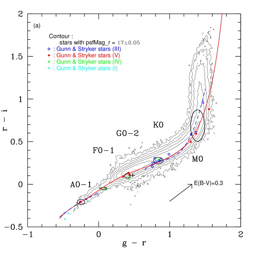
Figure 10: (a) Same as Figure 8 but in $r-i$ vs. $g-r$ plane.

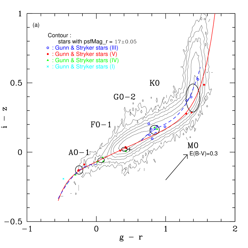
Figure 12: (a) Same as Figure 8 but in $i-z$ vs. $g-r$ plane.

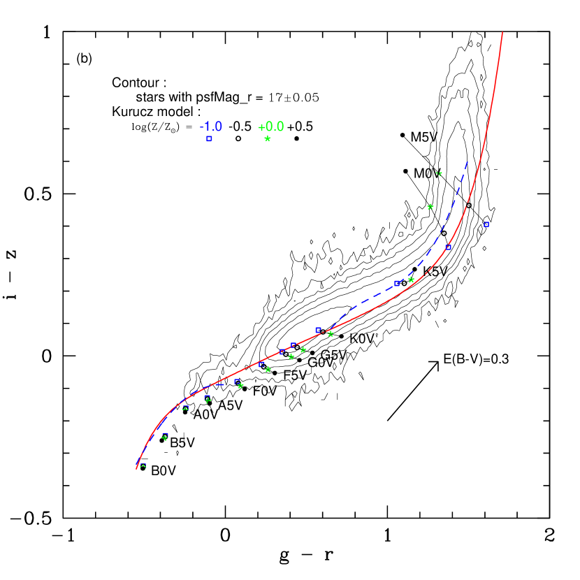
Figure 10: (b) continued

A similar figure is given for the $r-i$ vs. $g-r$ colour distribution in Figure 10. The splitting of tracks between luminosity classes III and V is very small: the two curves are nearly degenerate except for red stars with $g-r>1.2$. The variation due to metallicity is also reduced although it is still substantial in $g-r$. This generally smaller variation makes the discrepancy between the observation and the Kurucz atmosphere model, indicated by line segments in Figure 10b, somewhat more apparent. The Kurucz atmosphere model fits the curve representing the data only at its lowest metallicity edge, although the discrepancy is only about 0.03 mag in $r-i$. The trend is similar for the $i-z$ vs. $g-r$ colour distribution (Figure 12). We see a small gap appearing between the two luminosity classes which is somewhat more conspicuous than is seen in $r-i$ vs. $g-r$. Metallicity induced colour variation is larger for $i-z$, even larger than for $u-g$, for red stars.

All of the above indicates that the SDSS system is relatively close to a true AB system; the suspected corrections to an AB system of a few hundredths of a magnitude (Abazajian et al., 2009) are small enough not to have been seen in this analysis.

5 Colours of other objects

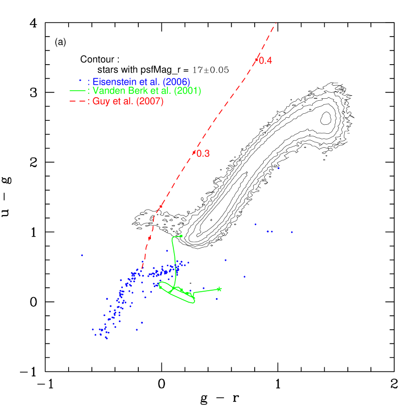
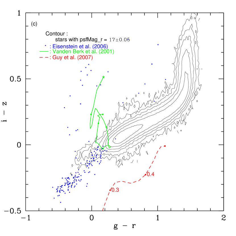
Figure 14: Distribution of stars in (a) $u-g$ vs. $g-r$ plane, (b) $r-i$ vs. $g-r$ plane, and (c) $i-z$ vs. $g-r$ plane (the same as Figure 2, 5 and 6, respectively, with isolated points representing individual stars suppressed). Small dots show hot white dwarfs. The solid curve shows the locus of quasars having the composite spectrum with redshift $\approx 0$ to 2.5, with blobs at the 0.5 interval in $z$: the lowest redshift is shown with the asterisk, which is $z=0$ for (a), $z=0.05$ for (b) and $z=0.35$ for (c). The dashed curve is the locus of Type Ia supernovae redshifted 0 to $z\leq 0.5$ towards red. The blobs on the supernova curve are at a 0.1 interval in redshift, but those at $z\approx 0$ is out of the range of the figure and omitted in (b) and (c). The blobs at $z=0.1$ and 0.2 are also omitted in (c).

To give the idea as to the feature of SDSS colours. we show in Figure 14 the distribution of white dwarfs, the sample of which is taken from the 9300 spectroscopically confirmed white dwarfs ($16.75<r<17.25$) of Eisenstein et al. (2006). They are white dwarfs with temperature typically $>7000$K. Cooler white dwarfs are degenerate with main sequence stars, and more with subdwarfs. Selections other than colours are needed to find candidates for cooler white dwarfs (Kilic et al., 2006; Harris et al., 2006). The locus of quasars is also added (solid curve) taking the composite spectrum of Vanden Berk et al. (2001) as the fiducial and by redshifting it to $z\leq 2.5$. The lowest redshifts shown depend on colour: they are 0 for $u-g$, 0.05 for $g-r$, and 0.35 for $r-i$. The locus of Type Ia supernovae at the epoch of their B-band brightness maximum is also shown (dashed curve) using the model spectrum of SALT2 (Guy et al., 2007) that is moved to non-zero redshift, $z\leq 0.5$. Some parts of the locii lie outside the frame of the figure.

The figure shows the distribution of white dwarfs well separated from normal stars due to their UV excess in the $u-g$ vs. $g-r$ plane, in so far as hot white dwarfs (approximately with $T>7000$K) are concerned, as efficiently used in Eisenstein et al. (2006), and to some extent also in the $i-z$ vs. $g-r$ plane. A strong degeneracy with normal stars is seen in the $r-i$ vs. $g-r$ plane. White dwarfs are degenerate with the blue tip of the distribution of normal stars with these colours.

Low redshift quasars, having $u-g$ colors much bluer than most stars, are also well separated from normal stars on the $u-g$ vs. $g-r$ plane till quasars reach $z\approx 2.5$, where they mingle into the stellar locus. The confusion of quasars with white dwarfs may take place in the $u-g$ vs. $g-r$ plane, though quasars are somewhat redder in $g-r$: this degeneracy is lifted if the $i-z$ vs. $g-r$ colour is used in addition. This demonstrates the advantage of multicolour space in the photometric selection of low redshift quasar candidates. The photometric target selection for quasars is discussed at length in the papers of Fan et al. (2001) and Richards et al. (2002, 2004), and we do not discuss this problem further.

The figure shows that Type Ia supernovae can be identified, well separated from the stellar locus, given the homogeneity of colours of Type Ia supernovae. The fiducial colour of the SALT II template at zero redshift, $u-g=0.476$, $g-r=-0.170$ and $r-i=-0.673$, is compared with that derived from the SDSS supernova sample, which reads $u-g=0.591\pm 0.237$, $g-r=-0.093\pm 0.157$ and $r-i=-0.636\pm 0.088$ where the error represents the sample variance (Yasuda & Fukugita, 2010). The diagram shows that Type Ia supernova locus moves monotonically with redshift, indicating that the photometric redshift can be estimated with a good confidence, given good colors at maximum light.

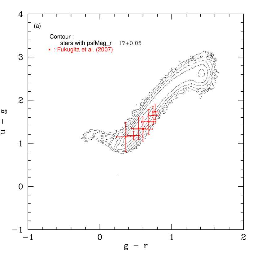
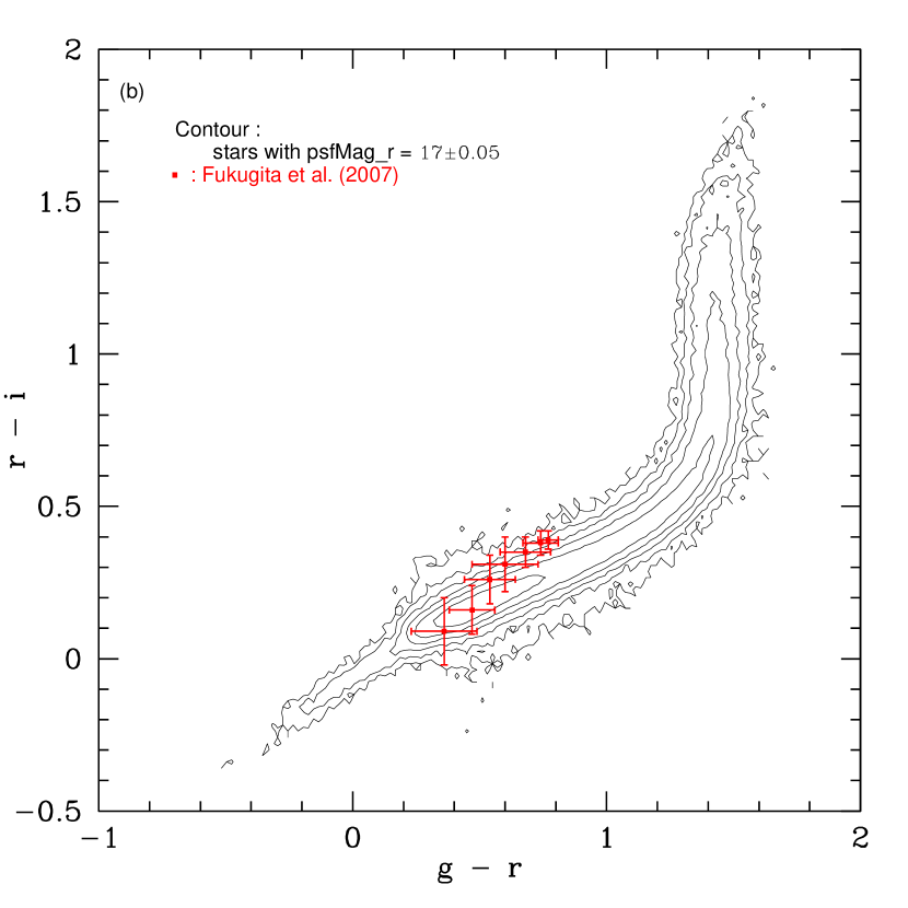
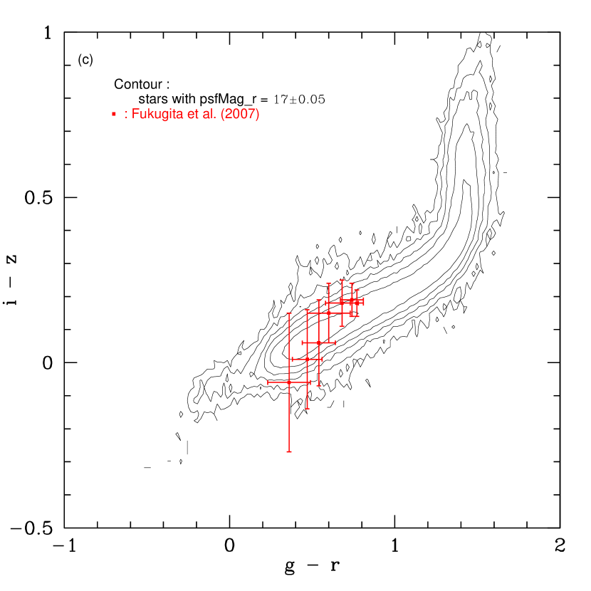
Figure 15: Distribution of stars in (a) $u-g$ vs. $g-r$ plane, (b) $r-i$ vs. $g-r$ plane, and (c) $i-z$ vs. $g-r$ plane, where colours of galaxies are overlaid. The error bars represent the variance of colours in the morphologically classified sample, from the right to the left E, S0, Sa, Sb, Sc, Sd and Im.

The three panels of Figure 15 show colours of morphologically classified galaxies at $z\approx 0$. Galaxy colours are taken from Fukugita et al. (2007) based on the visual classification of 2250 galaxies with $r\leq 16$ in the northern equatorial stripe. Magnitudes are Petrosian. The error bars indicate the variance of the samples for E, S0, Sa, Sb, Sc and Im. Galaxies occupy a colour space locus narrower than stars, with colours roughly corresponding to F5$-$K2 stars in the range $g-r=0.2-0.8$.

6 Brightness and colour of the Sun

The brightness of the Sun is taken as a basic unit in astrophysical work. The measurement of the brightness of the Sun, however, is notoriously difficult due to its extreme brightness and angular extent (e.g., Hayes, 1985). The measured broad band colour of the Sun has been variously reported from $(B-V)_{\odot}=0.62$ to 0.68 by various investigators. The choice often taken is $(B-V)_{\odot}=0.65$ (Allen, 1973).

We adopt the absolute spectrophotometry of the Sun measured by SOLSPEC in the Atmospheric Laboratory for Application and Science (ATLAS) 3 mission (Thuillier et al., 2003), the absolute flux of which has been calibrated against a black body standard. We present in Table 2 the synthetic broad band magnitudes of the Sun for $V$, $B-V$, $g$, $u-g$, $g-r$, $r-i$ and $i-z$. We take the $B$ and $V$ response functions evaluated by Ažusienis & Straižys (1969), which seem to give the minimal offset of synthetic brightness against Johnson broad band photometry among a number of response functions we tested (Fukugita, Shimasaku & Ichikawa, 1995). We also present synthetic values of brightness of the Sun using another spectrophotometric table compiled by Colina et al. (1996) in order to indicate the size of possible systematic errors.

The agreement among the different spectral energy distribution (SED) is within about 0.02 mag for the V band brightness. The SED of Thuillier et al. (2003) integrated with the reference response function of the SDSS 2.5m telescope with 1.3 airmasses, gives $V=-26.73$ mag which agrees well with $-26.75\pm 0.06$ mag of the summary value of photometry, given by Hayes (1985) and is also close to the value, $-26.74$, adopted in Allen’s Astrophysical Quantities (1973). The use of the SED from earlier missions of ATLAS also gives V band brightness within 0.02 mag of the ATLAS3 value. This is, in fact, the order of magnitude Thuillier et al. (2003) claimed as the error of calibration.

This result leads us to expect that solar SED can also be used to calculate broad band colours. The $B-V$ colour from Thuillier et al. (2003) is $0.62\pm 0.01$. While this looks somewhat bluer than the conventional value, we should remark that $B-V$ colour estimated from the colour temperature relations for main sequence stars with the solar abundance also lie bluer, in the range 0.616$-$0.635 (see Sekiguchi & Fukugita, 2000). The colour often quoted, $B-V=0.650$, is rather close to colour of G4 stars than G2, and is suspected to be too red.

The modern SED of the Sun gives a reasonable agreement among the different data sets for both absolute flux and colour. We calculate with a reasonable confidence $g-r$, $u-g$, $r-i$ and $i-z$ colour of the Sun as given in Table 2 in the AB₉₅ magnitude system. The $u-g$ and $g-r$ colours thus obtained (see the cross symbols in Figure 8) fall close to the later-type edge of the 1 $\sigma$ ellipse representing G0$-$G2 stars of the GS83 sample in Figure 8: $(u-g)_{\odot}=1.21$ and $(g-r)_{\odot}=0.45$ are close to the mean of two G2V stars in the GS83 sample, 1.22 and 0.43, respectively. The same is true also for the redder passbands: $(r-i)_{\odot}=0.13$ and $(i-z)_{\odot}=0.02$ are compared with 0.12 and 0.03 of the GS83 stars. The Sun thus matches very well with G2 stars. The brightness in the $g$ passband is $-26.46$. Our $V$ and $g$ magnitudes translate to absolute brightness $M_{V}(\odot)=4.84$ and $M_{g}(\odot)=5.11$ taking the distance modulus $-$31.57. For other colours, see Table 2.

7 Summary

We have studied photometric properties of stars given in the data archive of the SDSS, the primary question being whether the photometric calibration was, overall, properly done. We found that, over the entire lifetime of the survey, the photometric calibration for point sources has been made tightly against the SDSS standard stars and colours of the stars are well defined. We have not identified a sample of stars which are significantly and systematically deviant from the SDSS standard stars. We have also found that the synthesised colour from the Gunn Stryker spectrophotometric sample represents very well the colour of stars in the SDSS general catalogue and vice versa. Photometric properties are perfectly consistent mutually with each other among the three samples we studied. It is also gratifying that the the synthesis of the SDSS spectrophotometric data with the use of the reference response function of the 2.5m telescope of the SDSS give broad band fluxes that agree with broad band photometry of SDSS with little tilt along colours.

We have also given the fiducial colours and temperatures for stars empirically given spectral types, and show how metallicity and surface gravity affect colours. This enables us to infer spectral type of stars when SDSS colours is given. We show that $g-r$ colour can be used as a good estimator of the effective temperature of stars. The distribution of stars in colour space matches well with what we expect from the variations of metallicity and surface gravity. We also present the brightness and colour of the Sun with synthetic calculations, which shows that colour of the Sun matches well with G2V stars in the SDSS photometric system.

A problem we encountered in the present study is that the sample of stars with well known temperature and metallicity is still too scanty, and bright stars that have SDSS photometry are small in number. This is especially depressing when we require these two quantities at the same time. There is a pressing need to acquire photometry with the SDSS passbands for bright star samples which have good measured atmospheric parameters, (composition, temperature, and gravity) to connect more tightly SDSS photometry with physical stellar parameters.

Acknowledgement

We are grateful to Maki Sekiguchi and Takashi Ichikawa for their collaboration in our earlier work to define the AB system using the solar spectroscopic data (Sect. 5), and Masayuki Tanaka for his work measuring the response functions of the SDSS imager. We also thank David Hogg and Heather Morrison for a number of comments that helped us to tighten our results. MF is supported by the Monell Foundation at the Institute in Princeton, and received a Grant in Aid of the Ministry of Education (Japan) in Tokyo.

Funding for the SDSS and SDSS-II has been provided by the Alfred P. Sloan Foundation, the Participating Institutions, the National Science Foundation, the U.S. Department of Energy, the National Aeronautics and Space Administration, the Japanese Monbukagakusho, the Max Planck Society, and the Higher Education Funding Council for England. The SDSS is managed by the Astrophysical Research Consortium for the Participating Institutions. The Participating Institutions are the American Museum of Natural History, Astrophysical Institute Potsdam, University of Basel, University of Cambridge, Case Western Reserve University, University of Chicago, Drexel University, Fermilab, the Institute for Advanced Study, the Japan Participation Group, Johns Hopkins University, the Joint Institute for Nuclear Astrophysics, the Kavli Institute for Particle Astrophysics and Cosmology, the Korean Scientist Group, the Chinese Academy of Sciences (LAMOST), Los Alamos National Laboratory, the Max-Planck-Institute for Astronomy (MPIA), the Max-Planck-Institute for Astrophysics (MPA), New Mexico State University, Ohio State University, University of Pittsburgh, University of Portsmouth, Princeton University, the United States Naval Observatory, and the University of Washington.

Table 1: Temperature and colour of stars.

Type	$T_{\rm eff}$	$T_{\rm eff}$	$u-g$	$g-r$	$r-i$	Type	$T_{\rm eff}$	$T_{\rm eff}$	$u-g$	$g-r$	$r-i$
	colour	IRFM					colour	IRFM
B2V	(11195)		$-0.08$	$-0.50$	$-0.37$	B2III	(11180)		$-0.10$	$-0.50$	$-0.35$
B7V	(9631)		$0.49$	$-0.34$	$-0.25$	B7III	(9832)		$0.49$	$-0.36$	$-0.26$
A0V	8715		$0.98$	$-0.22$	$-0.19$	A0III	—
A5V	7656		$1.08$	$-0.04$	$-0.09$	A5III	7812	7997	$1.10$	$-0.07$	$-0,13$
F0V	—					F0III	—
F4V	6831		$1.11$	$0.13$	$-0.11$	F4III	—
F9V	5912	5902	$0.90$	$0.37$	$0.10$	F9III	—
G0V	6008		$1.04$	$0.34$	$0.09$	G0III
G2V	5747		$1.22$	$0.43$	$0.12$	G2III
G5V	5596		$1.29$	$0.48$	$0.14$	G5III
G8V	5217	5155	$1.51$	$0.62$	$0.21$	G8III	4969	5026	$1.86$	$0.72$	0.23
K0V	5610		$1.19$	$0.47$	$0.15$	K0III	4731		$2.14$	$0.84$	0.28
K4V	4600		$2.06$	$0.90$	$0.29$	K4III	4017	4050	$3.09$	$1.24$	$0.43$
K7V	3879	4011	$2.47$	$1.34$	$0.54$	K7III
M0V	(3793)		$2.44$	$1.41$	$0.66$	M0III	3828	3846	$3.16$	1.38	0.72
M2V	(3700)		$2.47$	$1.48$	$0.92$	M2III	(3585)		3.10	1.57	1.28
M5V	(3415)		$2.29$	$1.72$	$2.12$	M5III	(3576)		2.60	1.58	1.89

Note. — $T_{\rm eff}({\rm colour})$ is estimated from eq.(1) and the applicability is suspected for values given in parentheses; see the text.

Table 2: Brightness and colour of the Sun.

SED Data	$V$	$B-V$	$g$	$u-g$	$g-r$	$r-i$	$i-z$
Thuillier et al. (2003)	$-26.734$	0.622	$-26.459$	1.213	0.451	0.127	0.015
Colina et al. (1996)	$-26.748$	0.644	$-26.453$	1.234	0.479	0.106	0.020
	$M_{V}$		$M_{u}$	$M_{g}$	$M_{r}$	$M_{i}$	$M_{z}$
	4.84		6.32	5.11	4.66	4.53	4.52

Note. — Synthetic broad band absolute brightness obtained using Thuillier et al. (2003)’s SED. $V$ magnitude is in the Johnson system, giving $V=0.03$ for $\alpha$ Lyr. $ugriz$ magnitudes are in the $AB_{95}$ system.

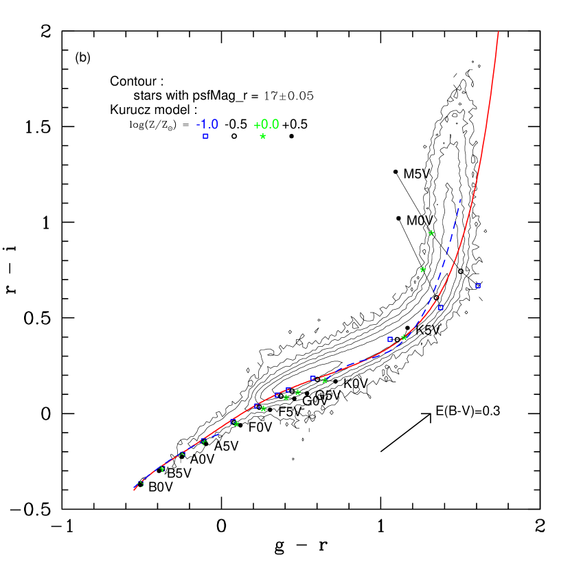
Figure 9: (b) continued

References

- Abazajian et al. (2003) Abazajian, K., et al. 2003, AJ, 126, 2081 (DR1)
- Abazajian et al. (2004) Abazajian, K., et al. 2004, AJ, 128, 502 (DR2)
- Abazajian et al. (2005) Abazajian, K., et al. 2005, AJ, 129, 1755 (DR3)
- Abazajian et al. (2009) Abazajian, K. N., et al. 2009, ApJS, 182, 543 (DR7)
- Adelman-McCarthy et al. (2006) Adelman-McCarthy, J. K., et al. 2006, ApJS, 162, 38 (DR4)
- Adelman-McCarthy et al. (2007) Adelman-McCarthy, J. K., et al. 2007, ApJS, 172, 634 (DR5)
- Adelman-McCarthy et al. (2008) Adelman-McCarthy, J. K., et al. 2008, ApJS, 175, 297 (DR6)
- Allen (1973) Allen, C. W. 1973, Astrophysical Quantities, 3rd edition, London: University of London, Athlone Press.
- Allende Prieto et al. (2008) Allende Prieto, C., et al. 2008, AJ, 136, 2070
- Ažusienis & Straižys (1969) Ažusienis, A., & Straižys, V. 1969, AZh, 46, 402
- Blackwell & Shallis (1977) Blackwell, D. E., & Shallis, M. J. 1977, MNRAS, 180, 177
- Castelli & Kurucz (2004) Castelli, F., & Kurucz, R. L. 2004, arXiv:astro-ph/0405087
- Cayrel de Strobel et al. (2001) Cayrel de Strobel, G., Soubiran, C., & Ralite, N. 2001, A&A, 373, 159
- Chen et al. (2001) Chen, B., et al. 2001, ApJ, 553, 184
- Cohen et al. (1978) Cohen, J. G., Persson, S. E., & Frogel, J. A. 1978, ApJ, 222, 165
- Colina et al. (1996) Colina, L., Bohlin, R. C., & Castelli, F. 1996, AJ, 112, 307
- di Benedetto (1998) Di Benedetto, G. P. 1998, A&A, 339, 858
- Doi et al. (2010) Doi, M., et al. 2010, AJ, 139, 1628
- Eisenstein et al. (2006) Eisenstein, D. J., et al. 2006, ApJS, 167, 40
- Fan et al. (2001) Fan, X., et al. 2001, AJ, 121, 31
- Fukugita, Shimasaku & Ichikawa (1995) Fukugita, M., Shimasaku, K., & Ichikawa, T. 1995, PASP, 107, 945
- Fukugita et al. (1996) Fukugita, M.,Ichikawa, T., Gunn, J. E., Doi, M., Shimasaku, K., & Schneider, D. P. 1996, AJ, 111, 1748
- Fukugita et al. (2007) Fukugita, M., et al. 2007, AJ, 134, 579
- Gray et al. (2001) Gray, R. O., Graham, P. W., & Hoyt, S. R. 2001, AJ, 121, 2159
- Gunn et al. (1998) Gunn, J. E., et al. 1998, AJ, 116, 3040
- Gunn et al. (2006) Gunn, J. E., et al. 2006, AJ, 131, 2332
- Gunn & Stryker (1983) Gunn, J. E., & Stryker, L. L. 1983, ApJS, 52, 121
- Guy et al. (2007) Guy, J., et al. 2007, A&A, 466, 11
- Harris et al. (2006) Harris, H. C., et al. 2006, AJ, 131, 571
- Hayes (1985) Hayes, D. S. 1985, Calibration of Fundamental Stellar Quantities, 111, 225
- Hogg et al. (2001) Hogg, D. W., Finkbeiner, D. P., Schlegel, D. J., & Gunn, J. E. 2001, AJ, 122, 2129
- Ivezić et al. (2004) Ivezić, Ž., et al. 2004, Astronomische Nachrichten, 325, 583
- Ivezić et al. (2008) Ivezić, Ž., et al. 2008, ApJ, 684, 287
- Kilic et al. (2006) Kilic, M., et al. 2006, AJ, 131, 582
- Kurucz (1993) Kurucz, R. 1993, SYNTHE Spectrum Synthesis Programs and Line Data. Kurucz CD-ROM No. 18. Cambridge, Mass.: Smithsonian Astrophysical Observatory, 1993
- Lee et al. (2008a) Lee, Y. S., et al. 2008, AJ, 136, 2022
- Lee et al. (2008b) Lee, Y. S., et al. 2008, AJ, 136, 2050
- Lenz et al. (1998) Lenz, D. D., Newberg, J., Rosner, R., Richards, G. T., & Stoughton, C. 1998, ApJS, 119, 121
- O’Donnell (1994) O’Donnell, J. E. 1994, ApJ, 422, 158
- Oke (1990) Oke, J. B. 1990, AJ, 99, 1621
- Oke & Gunn (1983) Oke, J. B., & Gunn, J. E. 1983, ApJ, 266, 713
- Padmanabhan et al. (2008) Padmanabhan, N., et al. 2008, ApJ, 674, 1217
- Pier et al. (2003) Pier, J. R., Munn, J. A., Hindsley, R. B., Hennessy, G. S., Kent, S. M., Lupton, R. H., & Ivezić, Ž. 2003, AJ, 125, 1559
- Richards et al. (2002) Richards, G. T., et al. 2002, AJ, 123, 2945
- Richards et al. (2004) Richards, G. T., et al. 2004, ApJS, 155, 257
- Schlegel et al. (1998) Schlegel, D. J., Finkbeiner, D. P., & Davis, M. 1998, ApJ, 500, 525
- Sekiguchi & Fukugita (2000) Sekiguchi, M., & Fukugita, M. 2000, AJ, 120, 1072
- Sesar et al. (2007) Sesar, B., et al. 2007, AJ, 134, 2236
- Smith et al. (2002) Smith, J. A., et al. 2002, AJ, 123, 2121
- Stoughton et al. (2002) Stoughton, C., et al. 2002, AJ, 123, 485
- Thuillier et al. (2003) Thuillier, G., Hersé, M., Labs, D., Foujols, T., Peetermans, W., Gillotay, D., Simon, P. C., & Mandel, H. 2003, Sol. Phys., 214, 1
- Tucker et al. (2006) Tucker, D. L., et al. 2006, Astronomische Nachrichten, 327, 821
- Vanden Berk et al. (2001) Vanden Berk, D. E., et al. 2001, AJ, 122, 549
- Yanny et al. (2009) Yanny, B., et al. 2009, AJ, 137, 4377
- Yasuda & Fukugita (2010) Yasuda, N., & Fukugita, M. 2010, AJ, 139, 39
- York et al. (2000) York, D. G., et al. 2000, AJ, 120, 1579