Rescaled potential for transition metal solutes in $\alpha$-iron

Abstract

We present empirical potentials for dilute transition metal solutes in $\alpha$-iron. It is in the Finnis-Sinclair form and is therefore suitable for billion atom molecular dynamics simulations. First principles calculation shows that there are clear trends across the transition metal series which enable us to relate the rescaling parameters to principal quantum number and number of $d$ electrons.

The potential has been developed using a rescaling technique to provide solute-iron and solute-solute interactions from an existing iron potential.

1 Introduction

The ability to model many component alloys of iron on the atomic level would provide an extremely powerful tool for research into the behaviour of these materials. In particular it would allow the effects of varying proportions of solutes on the properties of these materials to be studied in detail. The theoretical insights gained would complement the already extensive understanding of such systems found from experiment and ultimately impact on the design of new materials to suit particular applications such as those for the nuclear industry.

In principle one would wish to model these materials using ab-initio electronic structure calculations but such techniques are prohibitive, being restricted to less that 1000 atoms and femto second timescales. Alternative higher level modelling techniques exist, such as kinetic monte-carlo (kMC) and molecular dynamics simulations (MD) using empirical potentials, that remove these restrictions but at the expense of requiring input from experiment or ab-initio calculations to fix their free parameters. In particular, empirical potentials allow billion atom simulations to be performed over nano second timescales. The results from such simulations are readily used as input to continuum engineering models and ultimately in the design of new materials.

The Finnis-Sinclair scheme [1] was based around the idea of a second moment model to the local density of states. In this model the band energy depends on the width of the band, the shape of the band, and the occupation of the band. The moments theorem [2] shows how band width can be determined from the sum of squares of hopping integrals, which forms the physical basis for the cohesive term in Finnis-Sinclair potentials. The band shape and occupation are implicitly assumed to be constant.

For elements in a single phase with charge neutrality [3], the $d$-band occupation is essentially constant, and the band shape does not change massively. This underlies the success of single-element potentials. Fitting to alloys has a more troubled history. Whereas isoelectronic alloys for isostructural elements work well [4], potentials for systems involving structural phase transitions or elements from different series tend to have poor transferrability from the composition at which they are fitted. Thus the generalization to multicomponent alloys seems to require physics beyond the second-moment model. Difficulties also arise in the Finnis-Sinclair and related schemes such as the embedded atom method (EAM) [5, 6, 7] due to the increasing complexity of the model. For an $N$-component system the number of parameterised functions grows as $N^{2}$, as does the number of data points required to fit the parameters of these functions.

There is one important exception where the bandshape and electron density are reasonably constant, and we might hope that the second-moment approach will work. That is multicomponent alloys with one dominant element and multiple minority elements, a particularly relevant case here being steel. The dominant element fixes both the crystal structure and the electron density and should, in principle, connect the behaviour of single solute atoms to that of the dominant element and introduce stronger connections between solute-solute interactions and the properties of single solutes.

In this paper we present empirical potentials for single transition metal solutes in $\alpha$-iron by rescaling the functions of a pure iron potential. We also investigate ways to connect the interactions between solute particles to those of single solute atoms in iron which would allow multi-component potentials to be built once the interactions of single solutes in iron are known. We start by providing motivation for this procedure from the results of a recent ab-initio study [8] and then give a detailed description of the rescaling strategy. We then discuss the results for single solute atoms in iron and present the findings of our investigation into solute-solute interactions. Finally we present our conclusions.

2 Rescaling

2.1 Ab-initio calculations: Is rescaling credible?

If the key physics of substitutional atoms in steel is such that a rescaling approach will work, we should expect that the rescaling will involve the $d$-electron density and the principle quantum number. Such an approach should work both for the perfect lattice and for defects. The properties of substitutional transition elements in Fe, in particular their magnetic character, have long been known to have systematic trends [9, 10]. Here we supplement this work with an emphasis on total energy calculations for substitutional atoms and their interactions with point defects in bcc Fe.

We use the VASP code [11] with projector augmented wave (PAW) pseudopotentials [12] and the generalized gradient approximation [13] with the Vosko-Wilk-Nusair interpolation [14], which we find to give the best compromise between computation speed and accuracy. This gives a lattice parameter for pure iron of 2.83Å, which was used in the impurity and defect calculations to define a fixed-volume supercell. Supercells of 128 1 atoms were used with a Monkhorst-Pack 3x3x3 k-point grid sampling the Brillouin zone. The energy cutoff was set to 300 eV. Full details of the calculations will be published elsewhere [8].

The following definition has been used for the binding energy of $n$ defects and impurities, $\{A_{i}\}$:

$$E_{b}(\{A_{i}\})=\left[\sum_{i=1}^{n}E(A_{i})\right]-\left[E(\{A_{i}\})+(n-1)E_{0}\right],$$ (1)

where $E(A_{i})$ is the energy for a configuration containing $A_{i}$ only, $E(\{A_{i}\})$ refers to a configuration containing all the interacting entities and $E_{0}$ refers to a configuration containing no defects or impurities i.e. bulk $\alpha$-iron.

These total energy calculations show that there are systematic trends across the transition metal series for the free atom substitutional energy, $E_{s}$, excess pressure from a single solute, $P$, first nearest neighbour solute-iron separation, $r_{\mathrm{1nn}}$, solute-solute interactions, binding energies of a single solute to a vacancy defect at 1nn, $E_{\mathrm{b}}^{\mathrm{V,1nn}}$, and 2nn, $E_{\mathrm{b}}^{\mathrm{V,2nn}}$, separations and the binding energies to a $\langle 110\rangle$-self-interstitial defect in the mixed, $E_{\mathrm{b}}^{\mathrm{SI,M}}$, compressive, $E_{\mathrm{b}}^{\mathrm{SI,C}}$, and tensile sites ${}_{\mathrm{b}}^{\mathrm{SI,T}}$, (see FIG. 1 for configurations) as shown in FIG. 2. The free atom substitutional energy was calculated from our ab-initio results for the substitution energy from the pure equilibrium phase and the experimental cohesive energies of the pure phases [15]. We take these values as fit targets in order to determine the parameters of our potentials, as discussed in the following section.

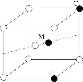
Figure 1: (a) First and second nearest neighbour solute sites (black) relative to a vacancy defect (square) (b) Mixed (M), compressive (C) and tensile (T) solute sites (black) relative to a $\langle 110\rangle$-self-interstitial defect.

We plot all energies against the number of $d$-electrons in the free atom. In the solid this number will be affected by $s-d$ transfer of approximately 0.5 electrons per atom. Thus although there are clearly different trends for more-than or less-than half filled bands, rigorously defining which material corresponds to a half-filled $d$-band is not straightforward.

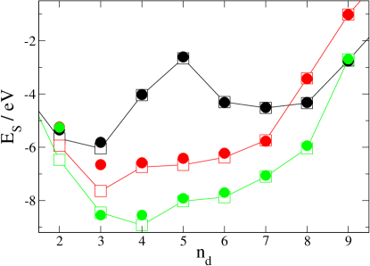
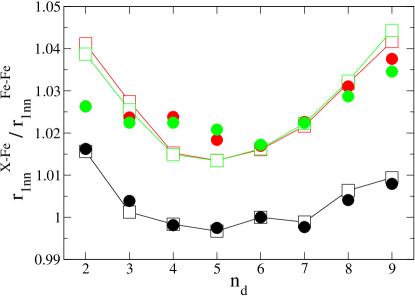
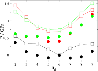
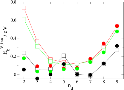
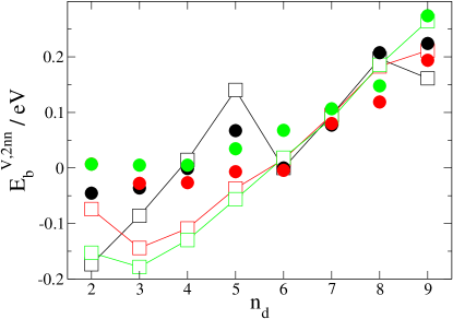
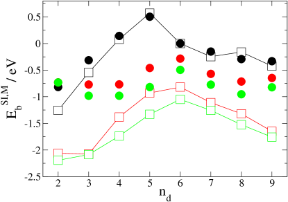
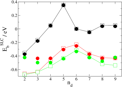
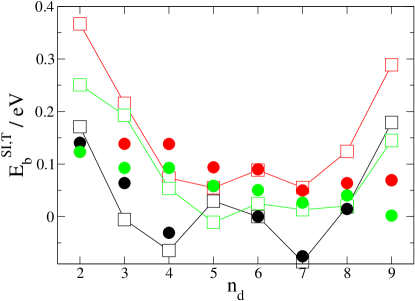
Figure 2: Fit targets (squares and lines) and corresponding values from our empirical model (circles) versus number of d-electrons for 3d solutes (black), 4d solutes (red) and 5d solutes (green). The first nearest neighbour solute-iron separation, $r_{\mathrm{1nn}}^{X-\mathrm{Fe}}$, is plotted relative to the corresponding iron-iron separation, $r_{\mathrm{1nn}}^{\mathrm{Fe-Fe}}$.

Two elements produce outlier behaviour: chromium and manganese. Curiously, iron chromium and manganese were elements which Finnis Sinclair were unable to fit with their original scheme [1]. These elements exhibit unusual magnetic behaviour, which presumably accounts for this.

2.2 Rescaling Strategy

The starting point for our fitting strategy is the pure iron EAM potential of Ackland et al. [16]. We have chosen this iron potential over those from more recent works [17, 18, 19] because it reproduces many of the properties of iron despite its relatively simple form.

The most general form for the energy, $U$, of an EAM potential is given by

$$U(\{r_{ab}\}) = \sum_{a,b>a}V^{(X_{a},X_{b})}(r_{ab})+\sum_{a}F^{(X_{a})}(\rho_{a}),$$ (2)

$$\rho_{a} = \sum_{b\neq a}\phi^{(X_{a},X_{b})}(r_{ab}),$$ (3)

where $V^{(X_{a},X_{b})}$, $\phi^{(X_{a},X_{b})}$ and $F^{(X_{a})}$ are parameterised functions dependent on the atomic species, $X_{a}$ and $X_{b}$. The cross-species pair functions are taken to be symmetrical here, i.e. $V^{(X,Y)}\equiv V^{(Y,X)}$ when $X\neq Y$, as are the functions, $\phi^{(X,Y)}$.

We use the same forms for the component functions of our potential as used in the pure iron potential [16]. In particular we define the pair functions by

$$V^{(X,Y)}(r)=\left\{\begin{array}[]{ll}\frac{Z_{X}Z_{Y}e^{2}}{4\pi\epsilon_{0}r}\xi(r/r_{s})&r\leq r_{1}\\ &\\ \exp(B_{0}+B_{1}r+B_{2}r^{2}+B_{3}r^{3})&r_{1}<r\leq r_{2}\\ &\\ C^{(X,Y)}(r)=\sum_{k=1}^{6}a_{k}^{(X,Y)}(r_{k}^{(X,Y)}-r)^{3}H(r_{k}^{(X,Y)}-r)&r>r_{2}\end{array}\right.$$ (4)

where $Z_{X}$ is the atomic number of species $X$, $r_{s}=0.88534\ a_{b}/\sqrt{Z_{X}^{2/3}+Z_{Y}^{2/3}}$, $a_{b}$ is the Bohr radius and

$$\xi(x)=0.1818e^{-3.2x}+0.5099e^{-0.9423x}+0.2802e^{-0.4029x}+0.02817e^{-0.2016x}.$$ (5)

The functional form used below $r_{1}=0.9$Å is the universal screened potential of Biersack and Ziegler [20], above $r_{2}=1.9$Å is a parameterised cubic spline with cutoffs implemented by the use of Heaviside step functions, $H$, and between these is an interpolating function that ensures continuity of the function and its derivative.

For the embedding functions, $F^{(X)}$, we take the standard square root form for all atomic species i.e. $F^{(X)}(\rho)=-\sqrt{\rho}$.

The $\phi$ functions take the form of a simple cubic spline

$$\phi^{(X,Y)}(r)=\sum_{k=1}^{2}A_{k}^{(X,Y)}(R_{k}^{(X,Y)}-r)^{3}H(R_{k}^{(X,Y)}-r).$$ (6)

For the pure iron component functions i.e. $V^{\mathrm{(Fe,Fe)}}$ and $\phi^{\mathrm{(Fe,Fe)}}$ we take the parameters directly from [16]. Iron-solute interactions are defined by rescaling these two functions using rescale parameters, $\{p_{i}^{(X)}\}$:

$$C^{(\mathrm{Fe},X)}(p_{1}^{(X)}r) = p_{2}^{(X)}C^{\mathrm{(Fe,Fe)}}(r)$$ (7)

$$\phi^{(\mathrm{Fe},X)}(p_{3}^{(X)}r) = p_{4}^{(X)}\phi^{\mathrm{(Fe,Fe)}}(r)$$ (8)

This is equivalent to a direct rescaling of the parameters of the cubic spline functions given by, for example,

$$r_{k}^{(\mathrm{Fe},X)} = p_{1}^{(X)}r_{k}^{\mathrm{(Fe,Fe)}}$$ (9)

$$a_{k}^{(\mathrm{Fe},X)} = \frac{p_{2}^{(X)}}{{p_{1}^{(X)}}^{3}}a_{k}^{\mathrm{(Fe,Fe)}}.$$ (10)

We take the rescaling factors, $\{p_{i}^{(X)}\}$, to be the adjustable parameters for the purposes of fitting. The trends in the fit target data should therefore translate to trends in these rescale parameters across the transition metal series. In fact it should be possible to quantify these trends by finding functional forms that relate the rescale parameters to the elementary electronic properties of the solutes. We present our results for the rescale parameters and a functional form for them in terms of the number of d-electrons per atom, $n_{d}^{(X)}$, in the following section.

Solute-solute interactions are defined by a similar rescaling procedure:

$$C^{(X,Y)}(p_{1}^{(X,Y)}r) = p_{2}^{(X,Y)}C^{\mathrm{(Fe,Fe)}}(r)$$ (11)

$$\phi^{(X,Y)}(p_{3}^{(X,Y)}r) = p_{4}^{(X,Y)}\phi^{\mathrm{(Fe,Fe)}}(r).$$ (12)

However, we do not determine these rescale parameters from fitting. Instead we relate them to the rescale parameters for the iron-solute interactions, i.e.

$$p_{i}^{(X,Y)}=p_{i}^{(X,Y)}(p_{i}^{(X)},p_{i}^{(Y)}).$$ (13)

This is the key step that ensures we can construct multi-component alloys once the iron-solute interactions are known.

3 Single solute interactions in iron

In order to determine the rescale parameters, $\{p_{i}^{(X)}\}$, we fit to the ab-initio data shown in FIG. 2 for transition metal solutes in $\alpha$-iron. We do not, however, fit to $E_{\mathrm{b}}^{\mathrm{SI,M}}$ as no satisfactory results were found with this quantity included.

The fitting procedure was accomplished by minimising a standard least squares response function, $\chi^{2}$, of the fit parameters, $\{p_{i}\}$, given in terms of the fit targets, $\{t_{r}\}$, model values, $\{m_{r}(\{p_{i}\})\}$, and weight factors, $\{\sigma_{r}\}$, by

$$\chi^{2}(\{p_{i}\})=\sum_{r}\left(\frac{m_{r}(\{p_{i}\})-t_{r}}{\sigma_{r}}\right)^{2}.$$ (14)

Our potential model values were all calculated in atomically relaxed 4x4x4 bcc unit cell configurations, i.e. 128 atoms before the introduction of defects and solutes, at the equilibrium volume for the pure iron potential, i.e. $a_{0}=2.8665\mathrm{\AA}$ [16]. This was done in order to appropriately match the ab-initio fit target data. We chose weight factors of 0.01eV (or $1\%$ of the fit target value if that is larger) for energies, $0.005\mathrm{\AA}$ for lengths and $5\times 10^{-4}$eV/$\mathrm{\AA}^{3}$ for pressures in our fits.

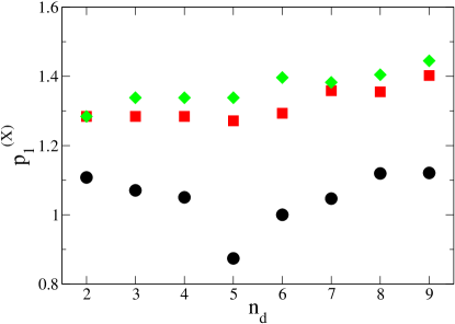
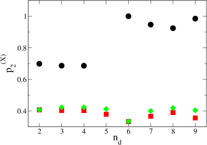
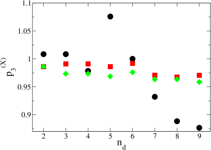
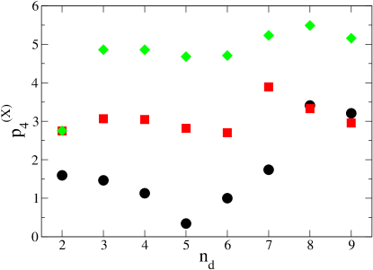
Figure 3: Rescale parameters as a function of the number of d-electrons for the 3d solutes (black circles), 4d solutes (red squares) and 5d solutes (green diamonds). The graphs are for (a) $p_{1}^{(X)}$, (b) $p_{2}^{(X)}$, (c) $p_{3}^{(X)}$ and (d) $p_{4}^{(X)}$.

The fitted rescale parameters are given in FIG. 3 and TABLE. 1. It it immediately clear that there are trends across the series, especially for the 4d and 5d transition metal solutes. The one notable exception is manganese whose anomalous rescale parameters match the equally anomalous properties of the solute itself.

Looking at FIG. 2 we can see that the trends in the rescale parameters translate to the potential model values themselves. There is especially good reproduction of the substitution energy across all three series. The binding energy, $E_{\mathrm{b}}^{\mathrm{SI,C}}$, is reproduced almost as well but shows slight deviation from the ab-initio target data at the ends of the series and especially for low $n_{d}$. Such deviations from the usually parabolic trends in the ab-initio data are seen generally for the other fit targets. The most notable is for the binding energy, $E_{\mathrm{b}}^{\mathrm{SI,T}}$, where the potential models show approximately linear behaviour in $n_{d}$. The overall deviations and the quality of the fits is best quantified via the response function values, as shown in TABLE. 2. It is clear from this data that the potentials for the low $n_{d}$ solutes perform especially poorly. This is an interesting results because the influence of s-electrons become increasingly important for these elements and their effects are not included in the pure iron potential we have rescaled here.

It is also clear from the response function data that the 3d solute potentials perform better overall than those of the other two series despite the presence of complex magnetic interactions. Even the anomalous properties of manganese are reproduced well. The excess solute pressures are, however, significantly underestimated although this is true of the 4d and 5d elements also.

Finally it is worth returning to the difficulties experienced in fitting the binding energy of the mixed interstitial, $E_{\mathrm{b}}^{\mathrm{SI,M}}$. As can be seen from FIG. 2 our potentials significantly underestimate the magnitude of this value for the 4d and 5d elements. Including this value in the fits did result in a more accurate reproduction but at too much cost to the reproduction of the other fit targets. Despite this the mixed site is still preserved as the least favoured for a solute to occupy around a $\langle 110\rangle$-self-interstitial defect. This failure is unlikely to have serious consequences for any molecular dynamics simulations using our potentials, since the mixed dumbbell site is not a migration barrier. The interstitial is repelled by the solute by well above any realistic thermal energy and so the mixed interstitial site will occur with very low probability.

4 Solute-solute interactions in iron

In order to gain some insight into the possible relationship between the solute-solute rescale parameters and the solute-iron rescale parameters we have fitted the rescale parameters, $\{p_{i}^{(X,X)}\}$, to reproduce ab-initio values [8] for the solute-solute binding energies from 1nn to 5nn separation, $E_{\mathrm{b}}^{X-X,i\mathrm{nn}}$, and to the separations between solutes at 1nn separation, $r_{\mathrm{1nn}}^{X-X}$, and 2nn separation, $r_{\mathrm{2nn}}^{X-X}$. The resulting values for the rescale parameters are shown in FIG. 4 and our model values are compared with the ab-initio fit targets in FIG. 5.

The fit targets in  FIG. 5 once again show a two-part trend across the group, which gives us hope that not only can rescaling be used to fit the potential functions directly, but also that the rescale parameters can be deduced directly from the atomic number. The picture emerging from the fit parameters themselves FIG. 4 is less clear. For elements above half-filling there are clear trends with principle quantum number and $n_{d}$. However, for 5d elements with $n_{d}<5$ there is considerable scatter for $p_{2}^{(X,X)}$ and $p_{3}^{(X,X)}$. It appears that for a longer-ranged $\phi$ can compensate for a stronger repulsion. since this anomaly is not present in the fit targets in FIG. 5, it must be an artifact of the fitting process itself.

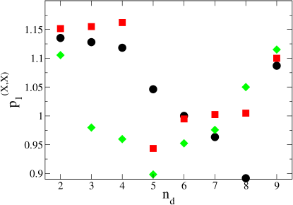
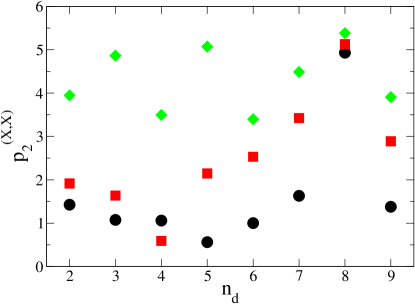
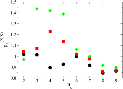
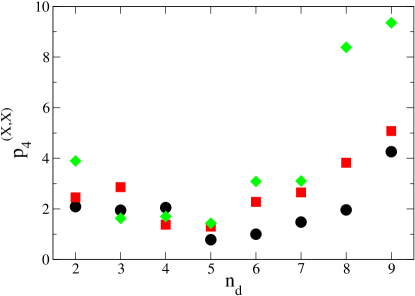
Figure 4: Rescale parameters as a function of the number of d-electrons for the 3d solutes (black circles), 4d solutes (red squares) and 5d solutes (green diamonds). The graphs are for (a) $p_{1}^{(X,X)}$, (b) $p_{2}^{(X,X)}$, (c) $p_{3}^{(X,X)}$ and (d) $p_{4}^{(X,X)}$.

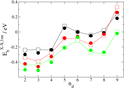
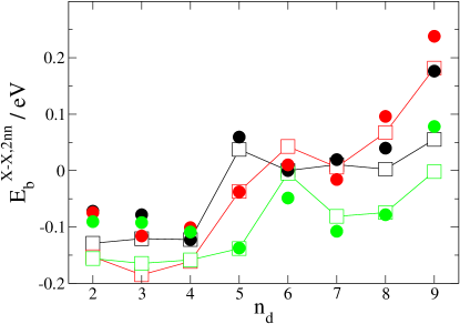
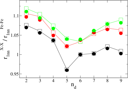
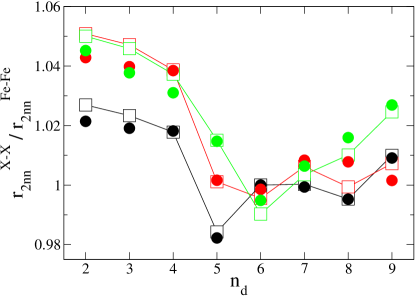
Figure 5: Solute-solute fit targets (squares and lines) and corresponding values from our empirical model (circles) versus number of d-electrons for 3d solutes (black), 4d solutes (red) and 5d solutes (green).

5 Conclusions

In conclusion, we have advanced the hypothesis that the interactions between transition metal atoms in iron can be described by simply scaling the parameters of a Finnis-Sinclair model, and further that these scaling parameters are simply functions of the number of $d$-electrons and the principal quantum number. Quantum mechanical calculations of interactions between solutes and point defect show clear trends across the group. We have presented best-fit rescaled potentials for all transition metal elements in an iron matrix.

Our hypothesis is based on the notion that the environment around the impurity is close to that in magnetic bcc iron, hence we do not expect that the rescaled potentials will be transferrable to very different electronic environments such as pure elements.

6 Rescale parameters for solute-iron interactions

Table 1: Rescale parameters for iron-solute interactions

Solute,$X$	$p_{1}^{(X)}$	$p_{2}^{(X)}$	$p_{3}^{(X)}$	$p_{4}^{(X)}$
Ti	1.1079352022752937	0.69914888963867840	1.0084290227415416	1.5946911193111377
V	1.0704687944688829	0.68703519774868570	1.0084191748980367	1.4652839386546592
Cr	1.0504446925177677	0.68660606895558630	0.9784540205196225	1.1287695242404665
Mn	0.8740657069080267	2.37899559818691970	1.0757805626557944	0.3418424453237209
Co	1.0467024050842750	0.94717978096230060	0.9320535734737820	1.7396896806120596
Ni	1.1194809316877880	0.92438826748289380	0.8883635622171985	3.4100636005122293
Cu	1.1208802828524023	0.98505124753645820	0.8765649836565008	3.2065254293566600
Zr	1.2841655075134310	0.40739377742609160	0.9860071367651349	2.7482154017401133
Nb	1.2841655075134310	0.40336016805208613	0.9909619464976229	3.0647879434909940
Mo	1.2841655075134310	0.40306261907883430	0.9909619275965241	3.0437240549628903
Tc	1.2714509975380506	0.37927270590314116	0.9860317313257698	2.8186046924493455
Ru	1.2932752539714167	0.33285431259332965	0.9918471983137220	2.7002031043018238
Rh	1.3583482886258411	0.36634462066369505	0.9706236772142814	3.8933887256877090
Pd	1.3551721040070680	0.39024726568702440	0.9674492344138608	3.3285717131180084
Ag	1.4023136316534160	0.35592505640677500	0.9705185530509607	2.9551289346288447
Hf	1.2841655075134310	0.40746747208599430	0.9860071367651349	2.7521572914348287
Ta	1.3381889417068988	0.42350948842405384	0.9734862986585047	4.8610714605878340
W	1.3381889417068988	0.42350948842405384	0.9734862986585047	4.8610567185373155
Re	1.3381889417068988	0.41247111384741486	0.9686430832422932	4.6812582679644960
Os	1.3963331257722620	0.33347841442944126	0.9760396335905974	4.7084791631263130
Ir	1.3825438675169937	0.40034598076904200	0.9633439996351745	5.2329577841196330
Pt	1.4045418753797260	0.41926814851469420	0.9633439996351745	5.4900896361876255
Au	1.4447702630891220	0.40420070742435266	0.9585272796369986	5.1583042920958950

Table 2: Response function values, $\chi^{2}$, for the best rescale parameters given in TABLE. 1.

Solute,$X$	$\chi^{2}(\mathrm{best})$
Ti	568.9656946430212
V	221.2048362240138
Cr	99.63599215304797
Mn	178.81158941110317
Co	43.901666493113794
Ni	65.72761363633806
Cu	204.8091878556158
Zr	4796.903769001561
Nb	1689.7527370510506
Mo	216.13918658727746
Tc	137.2039869893378
Ru	69.61819599245268
Rh	26.410945708888832
Pd	103.65177965112031
Ag	477.68739615717334
Hf	3491.8432724139166
Ta	1502.974429434891
W	408.3356703154182
Re	198.776262870386
Os	85.53222566998141
Ir	35.81070622123357
Pt	69.88189007267775
Au	386.0176534820233

References

- [1] M.W. Finnis and J.E. Sinclair, Phil. Mag. A 50, 45-55 (1984).
- [2] Ducastelle and Cyrot-Lackmann Adv.Phys 16, 393 (1967); J.Phys.Chem.Solids, 31, 1295 (1970)
- [3] G. J. Ackland, M. W. Finnis, and V. Vitek, J. Phys. F 18, L153 (1988).
- [4] G. J. Ackland, G. I. Tichy, V. Vitek, and M. W. Finnis, Phil. Mag. A, 56, 735 (1987).
- [5] M.S. Daw and M.I. Baskes, Phys. Rev. B 29, 6443-6453 (1984).
- [6] R.A. Johnson, Phys. Rev. B 39, 12554-12559 (1989).
- [7] G.J. Ackland and S.K. Reed, Phys. Rev. B 67, 174108 (2003).
- [8] P.Olsson, E.Vincent and C.Domain, in preparation
- [9] V.I. Anisimov, V.P. Antropov, A.I. Liechtenstein, V.A. Gubanov and A.V. Postnikov, Phys. Rev. B 37, 5598 (1988).
- [10] B. Drittler, N. Stefanou, S. Blügel, R. Zeller and P.H. Dederichs, Phys. Rev. B 40, 8203(1989).
- [11] G. Kresse and J. Hafner, Phys. Rev. B 47, 558 (1993); G. Kresse and J. Furthmuller, Phys. Rev. B 54, 11 169 (1996).
- [12] P.E. Blöchl, Phys. Rev. B 50, 17953 (1994); G. Kresse and D. Joubert, Phys. Rev. B 59, 1758 (1999).
- [13] J.P. Perdew et al., Phys. Rev. B 46, 6671 (1992).
- [14] S.H. Vosko, L. Wilk and M. Nusair, J. Can. Phys. 58, 1200 (1980).
- [15] J.D. Cox, D.D. Wagman and V.A. Medvedev, Codata Key Values for Thermodynamics, Hemisphere Pub. Corp., New York, (1989).
- [16] G.J. Ackland, D.J. Bacon, A.F. Calder and T. Harry, Phil. Mag. A 75, 713-732 (1997).
- [17] M.I. Mendelev et al., Phil. Mag. 83, 3977-3994 (2003).
- [18] G.J. Ackland, M.I. Mendelev, D.J. Srolovitz, S. Han and A.V. Barashev, J. Phys.:Condens. Matter 16, S2629-S2642 (2004).
- [19] M. Müller, P. Erhart and K. Albe, J.Phys.:Condens.Mater 19, 326220 (2007).
- [20] J.P. Biersack and J.F. Ziegler, Nucl. Instrum. Methods 194, 93-100 (1982).