Orbital structure in -Body models of barred-spiral galaxies
Abstract
We study the orbital structure in a series of self-consistent -body configurations simulating rotating barred galaxies with spiral and ring structures. We perform frequency analysis in order to measure the angular and the radial frequencies of the orbits at two different time snapshots during the evolution of each -body system. The analysis is done separately for the regular and the chaotic orbits. We thereby identify the various types of orbits, determine the shape and percentages of the orbits supporting the bar and the ring/spiral structures, and study how the latter quantities change during the secular evolution of each system. Although the frequency maps of the chaotic orbits are scattered, we can still identify concentrations around resonances. We give the distributions of frequencies of the most important populations of orbits. We explore the phase space structure of each system using projections of the 4D surfaces of section. These are obtained via the numerical integration of the orbits of test particles, but also of the real -body particles. We thus identify which domains of the phase space are preferred and which are avoided by the real particles. The chaotic orbits are found to play a major role in supporting the shape of the outer envelope of the bar as well as the rings and the spiral arms formed outside corotation.
keywords:
galaxies: structure, kinematics and dynamics, spiral.1 Introduction
The study of the orbits in barred galaxies begun in the late 70’s (Contopoulos & Mertzanides, 1977; Contopoulos, 1979) when the properties of the orbits in simple models of barred galaxies were derived theoretically by use of a ‘third integral’ of motion besides the Hamiltonian. Contopoulos & Papayannopoulos (1980) made an extended study of the periodic orbits in weak and strong bars, establishing the standard nomenclature thenceforward (see Papayannopoulos & Petrou (1983) and Contopoulos & Grosbol (1989) for a review of the various families of periodic orbits both inside and outside corotation). Many works have been devoted to the study of both periodic and non-periodic orbits in 2D (e.g. Athanassoula et al., 1983, 1990; Teuben & Sanders, 1985; Kaufmann & Patsis, 2005; Contopoulos & Patsis, 2006) or 3D models (e.g. Pfenniger, 1984; Pfenniger & Friedli, 1991; Patsis et al., 2002a, b, c, 2003a, 2003b). In most studies an ‘ad hoc’ choice of model is made for the gravitational potential. However, some studies have addressed the question of the orbital structure in -body systems of barred galaxies (e.g. Sparke & Sellwood, 1987; Sundin et al., 1993; Sundin, 1996; Barnes and Tohline, 2001; Shen & Sellwood, 2004; Ceverino & Klypin, 2007) in which, by definition, the orbits support the system self-consistently. Studies of the latter type are, in fact, necessary in order to identify which families of orbits are most relevant to the maintenance of self-consistency, i.e. to the production, by the orbits, of ‘response’ patterns matching those of the imposed potential/density field.
By constructing self-consistent models simulating real barred-spiral galaxies, Kaufmann & Contopoulos (1996) pointed out the role of the chaotic orbits in supporting the inner parts of the spiral arms emanating beyond the bar. The orbits considered by Kaufmann & Contopoulos belong to the so-called ‘hot population’ (Sparke and Sellwood 1987), i.e. they wander stochastically, partly inside and partly outside corotation. On the other hand, the same authors found that the outer parts of the spiral arms are supported mainly by regular orbits. The study of the role of the chaotic orbits in the spiral structure was pursued by Voglis et al. (2006a), using self consistent -body simulations of barred galaxies. These authors found long living spiral arms composed almost entirely by chaotic orbits. A new mechanism was proposed (Voglis et al., 2006b; Romero-Gomez et al., 2006, 2007; Tsoutsis et al., 2008; Athanassoula et al., 2008) according to which the invariant manifolds of the short period unstable periodic orbits around the stationary Lagrangian points and are responsible for the long-term support of the spiral structure. On the other hand Patsis (2006) argued that the innermost parts of the spiral arms, formed as a continuation of the bar, a little inside corotation, are due to chaotic orbits exhibiting, for long time intervals, a 4:1 resonance orbital behavior.
In Voglis et al. (2007) (hereafter paper I) a detailed investigation was made of the orbital structure in one system belonging to the series of -body experiments reported in Voglis et al. (2006a). This particular simulation represents a barred galaxy with nearly no spiral structure. Using i) the method of frequency analysis (Laskar 1990), and ii) 2D projections of the 4D surface of sections, obtained via the numerical integration both for test particles and of the real -body particles, the relative percentages were found of a number of distinct populations which support the bar. The analysis was carried out separately for the regular and the chaotic orbits. A significant fraction of chaotic orbits were found to lie inside corotation, thus supporting the shape of the bar. Moreover it was shown that in a 2D approximation in which the system’s thickness is ignored, the chaotic orbits are limited by tori or cantori so that many orbits remain confined inside limited domains outside corotation for times comparable to the Hubble time. Arnold diffusion through the third dimension was found ineffective over such time periods, thus the results are applicable in the 3D case as well.
In the present paper we extend the above study in the whole series of -body experiments reported in Voglis et al. (2006a), focusing in particular in those systems which simulate secularly evolving barred galaxies with significant spiral structure. The simulations represent self-consistent systems of a wide range of different pattern speeds of the bar. One main goal is to determine the dependence of the percentage of the different populations (particles in different types of orbits) on the value of the pattern speed. It should be stressed that the pattern speed of one system slows down as the system evolves secularly. To account for this effect, we study the orbital structure in each experiment at two distinct and well separated time snapshots, one close to the beginning of the simulation and one close to the final state (corresponding to one Hubble time evolution). This analysis yields the changes induced upon the different types of orbits, as well as upon the distributions of the -body particles in the orbital space, by the secular evolution of each galaxy towards an equilibrium state.
In order to accomplish the orbital classification, we implement the method of frequency analysis both for the regular and for the chaotic orbits of each system. The method of frequency analysis was first introduced in the study of bar like potentials (Binney and Spergel, 1982) and in the study of resonances between planetary orbits in the Solar system (Laskar, 1990), and within the framework of galactic dynamics it was implemented in the orbital study of elliptical galaxies (Papaphilipou & Laskar, 1996, 1998; Holley-Bockelmann et al., 2001, 2002; Kalapotharakos & Voglis, 2005; , 2007), or barred galaxies (Athanassoula, 2003; Martinez-Valpuesta et al., 2006; Voglis et al., 2007; Ceverino & Klypin, 2007). Here we extend the implementation of the method to the problem of spiral structure as well.
Besides identifying various types of regular orbits, concentrated around well known resonances, we find that many chaotic orbits, especially those being confined inside corotation, also exhibit a large degree of concentration around specific resonances. The main difference is that the chaotic orbits yield more diffused frequency maps than the regular orbits. Most chaotic orbits inside corotation can be further characterized as ‘weakly chaotic’, i.e. they have low values of the Lyapunov exponents. These orbits support the outer region of the bar. On the other hand, the chaotic orbits outside corotation are in principle capable of escaping. In most cases, however, the escape time is much longer than one Hubble time. Thus, in practice many chaotic orbits outside corotation are also trapped by various resonances exhibiting ‘stickiness’ along the invariant manifolds of the unstable periodic orbits near the Lagrangian points and . We demonstrate that the different populations of such orbits are responsible for practically all observed significant morphological features beyond the bar, and in particular for the observed rings and/or spiral arms.
Further examination of the phase space is performed using projections of the 4D surface of section of test particles. Using the same technique for the real -body particles, an important information is recovered, namely the location of those domains of the phase space which are preferred and those which are avoided by the real particles.
The paper is organized as follows. In section 2 we describe briefly the -body models and discuss the correlation between the pattern speed and the boxiness of the bar. In section 3.1 we present briefly the methods used for the classification of the orbits into regular and chaotic, we introduce the frequency analysis and we give the main results regarding the detailed orbital structure for all the models. In section 3.2 we examine the phase space structure through surfaces of sections using test particles as well as real -body particles. Finally section 4 summarizes the conclusions of the present study.
2 Description of the models
The series of simulations referred to in the sequel are described in detail in Voglis et al. (2006a). The experiments were evolved using the Smooth Field Code (hereafter SFC) of Allen et al. (1990). The initial conditions were created by introducing rotation in the so called ‘Q-model’ of Voglis et al. (2002) in the way described below.
A measure of the angular momentum , for a gravitational system of total mass M and total binding energy E, can be given in terms of Peebles’ (1969) ‘spin parameter’ :
| (1) |
The Q-model of Voglis et al. (2002) has initially an almost zero spin parameter, simulating an E7 elliptical galaxy (in contrast, the value of for, say, the disc of our Galaxy is , see Efstathiou & Jones, 1979). In fact, a value of close to the one observed in real barred-spiral galaxies cannot be obtained via a purely collisionless evolution of either a monolithically collapsing object, embedded in the tidal field of surrounding density perturbations, or a system formed by mergers between subclumps in a hierarchical clustering process. In order to produce systems with a parameter appropriate for barred galaxies, while running a collisionless simulation, Voglis et al. (2006a) introduced a process called ‘re-orientation of the velocities’. Starting from an equilibrium triaxial system (e.g. the Q-system), all the particles’ velocity vector components on the plane defined by the intermediate and long axes of the triaxial equilibrium figure are reoriented as to render each particle’s velocity vector perpendicular to its position vector. Furthermore, the re-orientation is such that the new velocity vector defines a clockwise sense of the particle’s orbital revolution. This process yields the maximum possible rotation of a system, on the above referenced plane, with respect to the progenitor system which has the same density and equal distribution of the velocity moduli. The experiment obtained from the Q-system via ‘velocity re-orientation’ was called QR1 (see Voglis et al., 2006a). This was left to run self-consistently, using an improved SFC version, for one Hubble time. In a similar way, the experiment QR2 was produced by introducing a new velocity re-orientation at a snapshot of the QR1 run corresponding to 20 half mass crossing times (hereafter ). The experiment QR3 was produced in the same way from QR2, and so on. We shall consider four -body experiments of this sequence (QR1 to QR4). All these experiments have the same number of particles () and the same binding energy but different amounts of total angular momentum, resulting therefore in different values of the bar’s pattern speed. Further details are provided in Voglis et al. (2006a). It must be pointed out here that in our self-consistent systems the particles cannot be identified a priori as belonging to a disc, halo or bulge component. The systems are flattened as a whole and when viewed edge-on they present a shape called ‘thick disc’ in Voglis et al. (2006a). The dynamical effects caused by the particles in the ‘thick disk’ were analyzed in details in Tsoutsis et al. (2008), in subsection 2.1, where it was shown that the particles with large vertical oscillations create a gravitational field which partly mimics the effect of a halo up to the code’s truncation radius. Moreover, it is possible to recognize even the bulge that is created self-consistently in barred galaxies, using a method proposed by observers, i.e. by plotting the density profile along and parallel to the major or minor axis of the bar. The bulge length is marked by the increased light distribution over the exponential disc, well above the bar (see Paper I for details).
In each experiment, the time unit is taken equal to the . A Hubble time corresponds to . The length unit is taken equal to the half mass radius (hereafter ). Finally, the plane of rotation is the plane (intermediate-long axes) and the sense of rotation is clockwise.
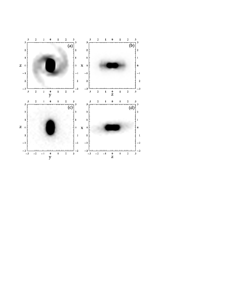
In Fig.1 the density of the particles of the experiment QR3 is plotted face-on (Fig.1a,c) and edge-on (Fig.1b,d), for two different snapshots (Fig.1a,b) and (Fig.1c,d). Some other snapshots of these four experiments in the ordinary space can be seen in fig.1 of Voglis et al. (2006a).
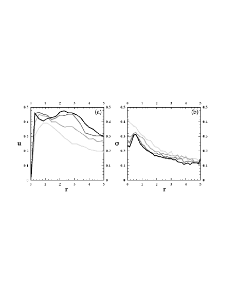
Figure 2a shows the rotation curves obtained by calculating the mean values of the line-of-sight velocity profiles of the particles when the systems are viewed edge-on and the bar is side-on (with the line of sight along the middle axis), for all the experiments from QR1 (light gray line) to QR4 (black line) at time . In Fig.2b the corresponding velocity dispersion profiles are plotted.
The slow down of the pattern speed in our experiments (see fig.4a in Voglis et al. 2006a) is smaller compared with other simulations using ‘live halos’ (see for example Athanassoula 2003 and Martinez-Valpuesta et al. 2006). Moreover, the evolution towards an equilibrium state seems faster. One possible reason is that, in our simulations, a bar already exists from the beginning of the calculations , where rotation has been inserted, via re-orientation of the velocities’ vectors, in all the particles of the system. Moreover, our systems present an important velocity dispersion especially in the central region (see Fig.2b) at time which is close to the initial conditions, and this favors the faster slow down of the bar’s pattern speed according to the main conclusion of Athanassoula (2003).
Apart from the QR1 experiment, in which the spiral structure does not survive for more that , in all the other experiments there are spiral modes surviving for 300 , i.e. for one Hubble time. The amplitude of these modes undergoes oscillations with an overall tendency to decay. However, during this secular evolution the spiral modes are more prominent at particular time snapshots. In all three models QR2, QR3 and QR4 the spiral structures are relatively strong at t=20.
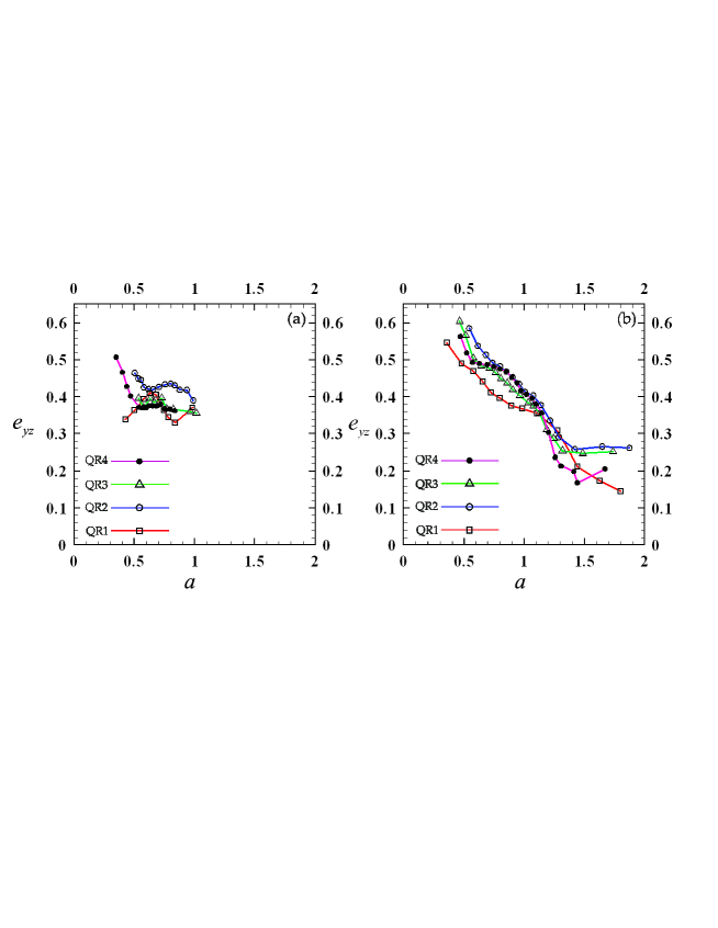
Figure 3 shows the ellipticity as a function of the major semi-axis of an isophote ( is the isophote’s minor semi-axis) for the isophotes corresponding to the projected surface density on the plane of each system. Fig.3a corresponds to an early snapshot far from equilibrium, while Fig.3b corresponds to , at which all systems have approached an equilibrium state. We see that, for , all the experiments present a nearly constant ellipticity along the bar, while, as the systems relax, the ellipticity profile acquires a declining slope, the isophotes becoming nearly round, i.e. the 3D matter distribution becoming nearly oblate beyond the end of the bar. The calculations for (Fig.3a) are limited within a radius because all the experiments, except QR1, present conspicuous spiral structures beyond this radius at so that the isophotes in this region cannot approximated by ellipses.
Boxiness of the isophotes is a well known feature in barred galaxies. This effect can be measured by the shape parameter , which can be determined by the equation of the generalized ellipse (Athanassoula et al. 1990):
| (2) |
where and are the major and minor semi-axes of an isophote and is the parameter describing the shape of a generalized ellipse best-fitting the isophote. For we obtain a standard ellipse, for the shape approaches a rectangular parallelogram and for we have a shape similar to lozenge.
| experiments | QR1 | QR1 | QR2 | QR2 | QR3 | QR3 | QR4 | QR4 |
|---|---|---|---|---|---|---|---|---|
| snapshots | ||||||||
| 0.4 | 0.36 | 0.7 | 0.46 | 0.82 | 0.52 | 0.96 | 0.59 | |
| % chaotic motion | 59.6 | 57.9 | 61.8 | 57.3 | 63.0 | 59.4 | 56.6 | 56.4 |
| % chaotic motion inside corotation | 28.5 | 27.8 | 12.6 | 16.0 | 9.8 | 14.9 | 7.4 | 11.1 |
| % regular motion (2:1) | 12.6 | 16.5 | 18.4 | 21.9 | 14.9 | 17.8 | 21.6 | 21.2 |
| % regular motion (3:1) | - | - | 18.7 | - | 19.8 | - | 18.5 | - |
| % regular motion (A) | 25.5 | 20.4 | - | 15.8 | - | 21.5 | - | 20.8 |
| % regular motion (B) | - | 4.0 | - | 2.6 | - | 1.1 | - | 1.2 |
| % chaotic motion (2:1) | 1.8 | 8.7 | 1.7 | 2.7 | 1.3 | 2.0 | 1.1 | 1.7 |
| % chaotic motion (3:1) | 5.4 | 4.7 | 5.6 | 3.7 | 5.0 | 3.7 | 4.5 | 3.0 |
| % chaotic motion (4:1) | 4.2 | 6.5 | 4.3 | 4.4 | 4.2 | 1.5 | 3.1 | 2.7 |
| % chaotic motion (A) | 4.8 | 12.4 | - | 9.7 | - | 7.9 | - | 6.0 |
| % chaotic motion (cor) | 6.2 | 6.4 | 2.9 | 2.6 | 2.5 | 1.7 | 2.6 | 2.1 |
| % chaotic motion (-2:1) | 2.4 | 3.2 | 2.4 | 1.7 | 2.5 | 0.7 | 3.1 | 0.6 |
| % chaotic motion (-1:1) | - | 2.0 | - | 2.3 | 4.4 | 1.9 | 4.4 | 2.1 |
| % chaotic motion () | 14.8 | 8.7 | 30.0 | 23.1 | 35.2 | 33.4 | 26.1 | 35.7 |
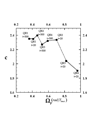
Fig.4 shows the shape parameter as a function of the pattern speed of the bar at the time snapshots specified within the figure for each experiment. Each point’s ordinate corresponds to the mean value of the parameter of the generalized ellipses having major semi-axis between and , where is the system’s corotation radius at the indicated snapshot. The abscissa of each point corresponds to the associated pattern speed of the bar. For values of smaller that the corresponding -parameter seems to have a flat behavior with . However, for values greater than a declining relation is apparent indicating that the boxiness decreases as the pattern speed increases. Similar study for elliptical galaxies has been presented in Naab et al. (1999); Gonzalez-Garcia et al. (2006).
3 Study of the orbital structure
3.1 Frequency analysis of the orbits
The distinction of the regular from the chaotic orbits is based on a combination of two methods, namely the Specific Finite Time Lyapunov Characteristic Number (SFTLCN) or simply , introduced by Voglis et al. (2006a), and the Smaller ALignment Index, (SALI), or simply Alignment Index () (Skokos, 2001; Voglis et al., 2002). For more details on the implementation and efficiency of these combined methods see Paper I.
The percentage of chaotic orbits in all the experiments is close to (see Table 1), which is almost twice the corresponding percentage found in the non-rotating progenitor model, i.e. the Q-model (Voglis et al., 2002). The general conclusion in Voglis et al. (2006a) is that rotation enhances chaos, not only as regards the fraction of mass in chaotic motion, but also as regards the magnitude of the Lyapunov numbers that are seriously shifted towards higher values. The authors argued that rotation introduces instabilities and a sequence of important overlapping resonances between the pattern speed and the frequencies of orbits. This fact is imprinted in the increase of the chaotic motion. The same conclusion has been reached in other studies dealing with orbits in bar like galaxies. For example, Quillen (2003), noted that an increase of the pattern speed of the bar model simulating the Milky way increases significantly the chaotic regions on the Poincaré map because of resonance overlap phenomena. Also, Berentzen et al. (2001), found that the combination of a triaxial halo with a fast-rotating bar leads to the development of chaos. Finally, Muzzio (2006) found that the fraction of the chaotic orbits is enhanced in triaxial stellar systems when rotation is inserted. However, in all the experiments the fraction of mass that can develop effective chaotic diffusion within a Hubble time is less than (fig.12b in Voglis et al., 2006a) which means that a significant percentage of orbits are weakly chaotic.
In the experiment QR1 there appears a transient trailing spiral structure as a result of the transfer of angular momentum to the material outwards (Lynden-Bell & Kalnajs, 1972; Tremaine & Weinberg, 1984; Weinberg, 1985; Athanassoula, 2003). The transient spiral arms disappear quickly (after ). As a result, the system resembles a bar-like galaxy without any spiral structure. The orbital analysis of this experiment at was the subject of Paper I.
Here, we exploit the tool of frequency analysis (Laskar, 1990; Papaphilipou & Laskar, 1996, 1998) using the improved code of Sidlichovsky & Nesvorny (1997). We apply this technique separately for the regular and the chaotic orbits in all four experiments and for two different snapshots corresponding to 20 and 300, respectively. In order to obtain the frequency analysis of the orbits at one snapshot, all the orbits are integrated forward in the ‘frozen’ potential corresponding to that snapshot, and for a time equal to 150 radial periods. The Jacobi constant of one orbit is given by the relation
| (3) |
where is the full 3D ‘frozen’ potential, given by the SFC code as an expansion of a bi-orthogonal basis set, are the velocities in the rotating frame of reference and is the angular velocity of the bar at the studied snapshot (see Table 1 for the values of for all the models in the two snapshots). The value is the distance from the rotation axis.
The integrated orbits belong in a wide range of Jacobi integral values which implies a wide range of orbital periods (e.g. radial periods) of each orbit. This means that within a certain time (e.g a Hubble time) each orbit has a quite different dynamical evolution. In order to treat this integration process with the minimum computational cost, we have used a Runge-Kutta 7(8) order integrator with variable time step. This technique guaranties a relative error of the Jacobi constant less than for all the integrations we provide below. Moreover, by requiring a relative error less than we obtained very similar results, which implies that the presented results are robust.
By running the orbits in the ‘frozen’ potential, we then calculate the following frequencies for each orbit:
a) the radial frequency (frequency of epicyclic oscillations) which is derived from the time series of the radial velocity
b) the angular frequency in the rotating frame of reference, , or the inertial frame, , which are derived from the time series of the corresponding polar angle
c) the vertical frequency, which is derived from the time series of the coordinate .
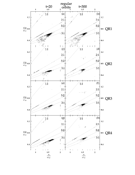
The main resonances can now be detected using frequency maps. Figure 5 shows the rotation numbers of the ensemble of regular orbits for all the experiments at the two studied snapshots. Each row (column) of panels corresponds to a different system (snapshot) as indicated in the figure. In each panel, one point corresponds to one orbit of a real -body particle that turns to be regular. In the ‘frozen potential’ approximation the position of this point on the plane remains invariant in time, since the particle’s orbit stays confined on an invariant torus with the given values of the rotation numbers.
The most important resonances are the ‘disc’ resonances which are of the form , with integers. Such resonances are shown by gray straight lines in Fig.5. Orbits lying exactly on them belong to two groups:
a1) if no second resonance relation of the form , with all three integers , is satisfied, the orbit lies on a torus of dimension smaller than or equal to three. The orbit is quasi-periodic, and it is the product of a vertical oscillation and of a motion on the plane which is either exactly periodic or a ‘tube’ around a planar periodic orbit. The motion in the third dimension is essentially decoupled from the motion on the 2D plane. In practice, we find that the great majority of -body particles in exactly resonant orbits populate precisely the above group. Furthermore, most of them exhibit vertical oscillations of a rather small amplitude, compared to the motion on the plane (this is expected since the system as a whole is substantially flattened in the -axis). Thus a study of dynamics via a 2D approximation is sufficient to unravel all interesting properties of such orbits.
a2) if a second resonance relation of the form is satisfied, the orbits are called ‘doubly resonant’. The orbits can be exactly 3D-periodic, corresponding e.g. to a vertical bifurcation from the x1 family (see Skokos et. al 2002 for a classification and nomenclature of such periodic orbits), or thin tubes around these periodic orbits. Particles on such orbits influence mainly the ‘edge-on’ profiles of our systems. The study of these orbits is outside the scope of the present paper and will be undertaken in a separate study. The connection between the ‘disc’ resonances and the orbital frequencies is explicitly defined, in Athanassoula (2003).
On the other hand, particles satisfying a ‘disc’ resonance relation only approximately, i.e.
| (4) |
can also be distinguished in two cases:
b1) if there is one exact resonance relation of the form , , the orbit lies on an invariant 2D torus. When projected on the plane, however, the orbit is not captured in the associated disc resonance, i.e., it lies entirely outside the separatrix domain corresponding to that particular resonance under a 2D approximation of the dynamics. Such orbits exhibit a slow precession around the associated exact disc resonances and they are responsible for a number of interesting features of the ‘face on’ appearance of the galaxies, examined in detail below.
b2) if there is no exact resonance relation of the form the orbit is quasi-periodic, lying on a 3D torus. When projected on the plane, these orbits share most features of the orbits of group (b1).
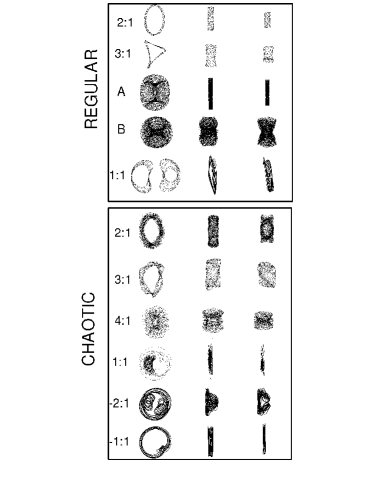
In Fig.5, we observe that the majority of particles in regular orbits are concentrated along and around specific resonance lines. A very clear concentration is seen along the resonance 2:1 (that corresponds to and in Eq.4). These are quasi-periodic orbits forming thin tubes around the ‘x1’ type of periodic orbits (Contopoulos & Papayannopoulos, 1980) at values of the Jacobi constant corresponding to distances near the inner Lindblad resonance (hereafter ILR). Both the periodic and quasi-periodic orbits of this type have ellipsoidal forms in the 3D space, which are projected to elliptical figures in the plane with a long axis aligned to the long axis of the bar (Fig.7).
The 2:1 is the main resonance supporting the bar and therefore it is well populated in all four experiments both at 20 and at 300. On the other hand, depending on the system and snapshot considered, other significant groups of regular orbits supporting the bar are distinguishable. We note that the simple resonances of the form , , implying epicyclic per one azimuthal oscillation, are concentrated, as increases, to domains of the phase space (or values of the Jacobi constant) closer and closer to corotation. Since the accumulation of these resonances causes chaos by the mechanism of resonance overlap (see Contopoulos 2002 p.185), the regular orbits are expected to lie at resonances with a low value of , or some nearby non-simple resonances , while the chaotic orbits fill the remaining parts of the resonance web, i.e. the simple resonances with high values of or their nearby non-simple resonances .
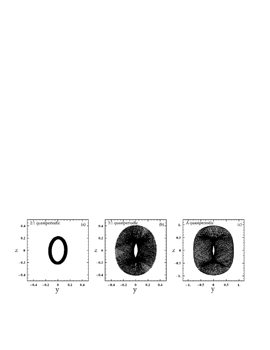
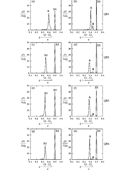
Figure 6 gives the distribution of regular orbits along the quantity calculated for all the systems at 20 (left hand column) and at 300 (right hand column). Note that the pattern speed of the bar at any snapshot can be derived from fig.4a of Voglis et al. (2006a). It is well known that the quantity distinguishes very efficiently the various resonances and it has been used for the orbital classification in previous studies (e.g. Athanassoula, 2003; Ceverino & Klypin, 2007).
Each peak in Fig.6 corresponds to the indicated population. Besides the ILR (at ) we identify other important peaks in the -value distribution of the -Body particles. One prominent peak which appears at early snapshots (except in the experiment QR1) is at the 3:1 resonance (that corresponds to and in Eq.(4) and to in Fig.6). This peak nearly disappears at late snapshots, being replaced, instead, by a different peak, called hereafter group ‘A’. This corresponds to particles with a -value . This population has been found in other -body simulations of bar-like galaxies (see for example Martinez-Valpuesta et al., 2006; Ceverino & Klypin, 2007). The transition from a distribution peaked at the 3:1 resonance to a distribution peaked at the group ‘A’ is related to a morphological transition in the bar, discussed in detail below.
A less populated group called group ‘B’, is also observed at snapshots near equilibrium (e.g. ). This consists mainly of quasi-periodic retrograde orbits with a projection of the ‘x4’ type (Contopoulos & Papayannopoulos 1980), i.e. elongated perpendicularly to the bar and correspond to and in Eq.(4). Remarkably, many orbits of this group exhibit also vertical oscillations (see Fig.7). The group ‘B’ orbits cannot exist at snapshots close to the beginning of the simulation, as for example , since the ‘velocity re-orientation’ process, by which the initial conditions are produced, implies that there be no retrograde orbits initially. Thus the group ‘B’ population develops in the course of the simulation, as the systems evolve towards the equilibrium. From the right panels of Fig.6 we can conclude that the number of particles in the group ‘B’ decreases with increasing pattern speed (e.g. from QR1 to QR4). This is further substantiated in section 3.2 in which we show that in all the self-consistent systems the phase space corresponding to the ‘x4’ family is almost empty.
Finally, in the experiment QR1, which does not have any spiral structure, there is a small concentration of particles in regular orbits along the resonance line 1:1 (see Fig.5). This resonance corresponds to the short period orbits PL4 and PL5 (using the nomenclature of Voglis et al. 2006b for the short period periodic orbits, bifurcating from the corresponding Lagrangian points), around the Lagrangian points and (see Fig.7) and exists for values of the Jacobi constant close to the one at corotation. In all the other experiments there are no regular orbits of this type.
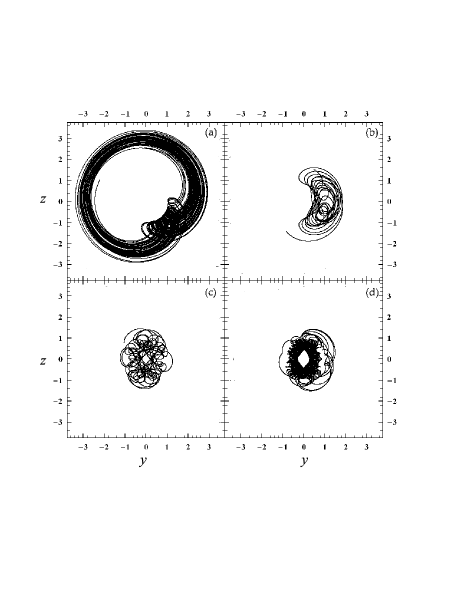
The implications of the transition from a 3:1 peak at early snapshots to a group ‘A’ peak at late snapshots can be discussed with the help of Figs.7 and 8. Figure 7 shows the projections on various planes of some regular orbits trapped in major disc resonances. It is obvious that the group ‘A’ orbits yield a ‘boxy’ form, while the resonant 3:1 orbits are asymmetric with respect to the bar’s major axis (we can find a different orbit, symmetric to the 3:1 orbit of Fig.7, with respect to the axis of symmetry ). However, other orbits of the group of Fig.6, which are selected so that they are not exactly resonant (i.e. ), exhibit a precession of the apocentres which corresponds to a motion in the phase space close to, but outside the separatrices marking the 3:1 resonant domain. Such an orbit is shown in Fig.8b. Orbits such as in Fig.8b are considerably less boxy than the orbits of group ‘A’ (Fig.8c), although they are more boxy than the 2:1 resonant orbits (Fig.8a). We conclude that if the peak of the distribution is pronounced compared to other peaks, the bar isophotes appear more ‘disky’, i.e lower values (see Fig.4 for the early snapshots of the experiments QR2 to QR4). On the contrary, the enhancement of group ‘A’ orbits is responsible for the ‘boxy’ isophotes (high values in Fig.4) at the late snapshots of the same experiments. This implies also a correlation between the position of the peaks of the -distribution and the value of the pattern speed of a particular galaxy. The 3:1 type of orbits appears mainly in systems with a high value of (e.g. the systems QR2, QR3, QR4 at ), while, as the systems slow down, the peak becomes gradually depleted and, instead, the -body particles gradually populate the group ‘A’ type of orbits, which, hence, becomes a dominant type in systems with a low value of (QR2, QR3, QR4 at ). Note that the pattern speed of the QR1 experiment is quite small already at , and, in this particular experiment, the group ‘A’ peak is prominent also at this snapshot. This discussion suggests that is indeed, the relevant parameter to which the position of the main peaks of the -distribution should be correlated.
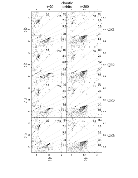
Figure 9 shows the frequency maps of the chaotic orbits, for all the systems and for two different snapshots as indicated in the figure. It is obvious that the chaotic orbits appear quite scattered in these diagrams. Nevertheless, many chaotic orbits are trapped near various resonance lines. Such orbits are called ‘sticky’ and they behave similarly to regular orbits for long times. An interesting remark is that there are chaotic orbits near resonance lines where no regular orbits are observed. For example, in Fig.9 we can see points around the 3:1 and the 4:1 resonance as well as around the 1:1 resonance (see Fig.7 for their shapes), at snapshots when there are only a few regular orbits in these resonances (compare Figs. 5 and 9).
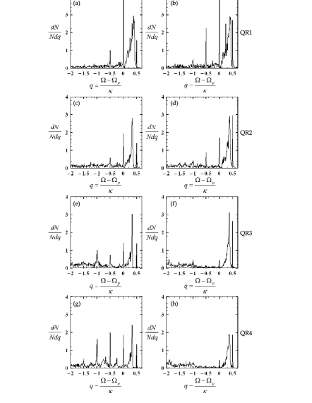
Figure 10 shows the distribution of the values for the chaotic orbits of all the systems. The first remark is that the chaotic orbits are distributed in a greater variety of -values than the regular ones. The -distributions present peaks at the same values of as for the regular orbits. Nevertheless, important peaks appear also at other resonances, as seen in the figure. Note that corotation, ILR and outer Lindblad resonance (hereafter OLR) correspond to and values of , respectively. In general orbits located inside (outside) corotation have positive (negative) values. The orbits corresponding to smaller values reach larger distances on the plane. Since at all the systems have lower values than at , the corotation radius is at larger distances. This explains the smaller percentage of orbits found outside corotation () at .
The percentages of the most important populations of regular and chaotic orbits, derived from Figs.6 and 10, are given in Table 1.
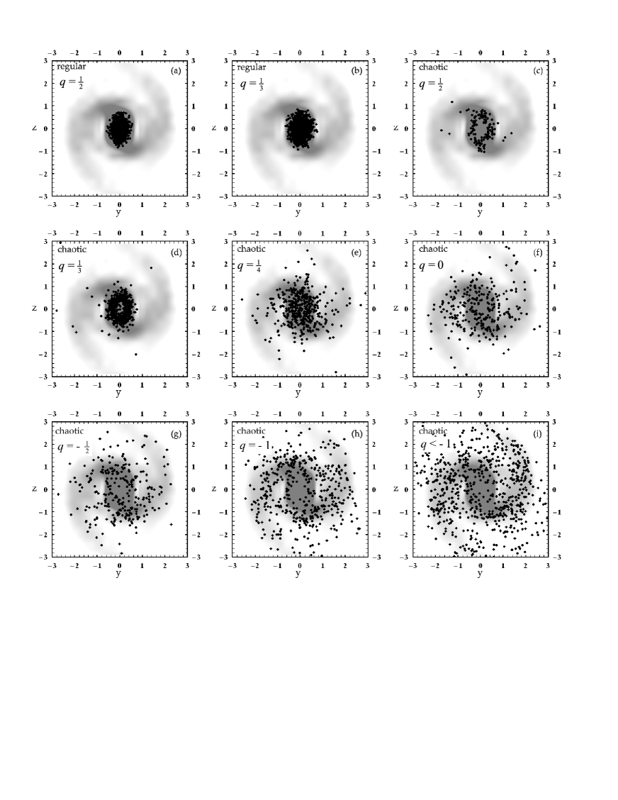
We now come to see the role of the various populations in supporting particular morphological features of the studied systems. In subsequent plots we focus on one example, the QR3 experiment, which exhibits all interesting phenomena. The ‘backbone’ of the system, i.e. its appearance on the plane, is plotted as a gray background in a number of subsequent plots.
Figure 11 shows the ‘backbone’ of the system QR3 at together with the instantaneous positions of the particles belonging to the various identified populations of regular and chaotic orbits. The backbones of QR2, QR3 and QR4 are similar at . All four experiments present a bar, two spiral arms and a faint ring. We observe that the regular orbits contribute to the form of the bar. On the contrary, the chaotic orbits support the structures both inside and outside corotation. The chaotic orbits inside corotation () create an envelope of the bar, the particles being located at the outer bar layers. Similar orbits were found in Patsis et al. (1997). The particles in chaotic orbits near the 4:1 resonance () support segments of the spiral arms connected to the bar. The population corresponding to corotation contributes to the outer bar as well as to the ring. The chaotic orbits located near the OLR , as well as near the resonance , contribute to the ring and to the spiral arms. The chaotic orbits below the resonance contribute mainly to the spiral arms.
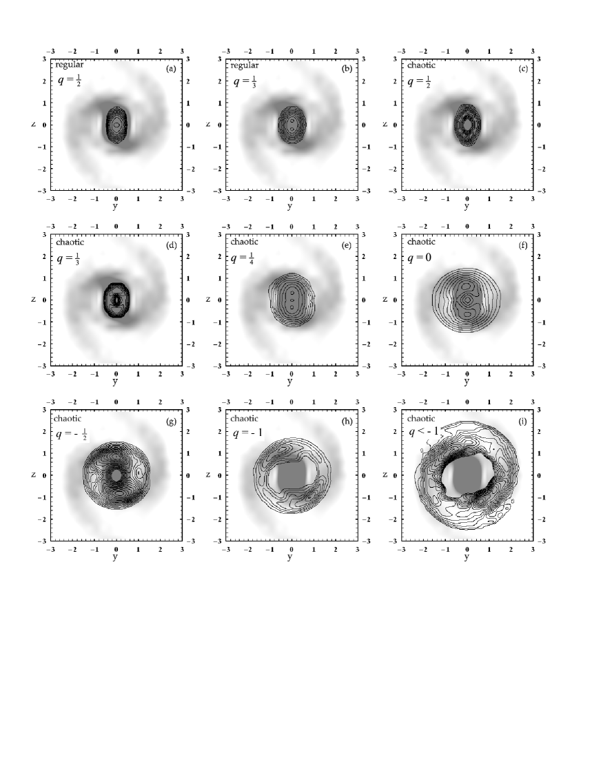
In Fig.11 we only see which features of the system are supported by the instantaneous positions of the particles. Thus we have no information about the trend for morphological changes induced by the chaotic orbits undergoing slow chaotic diffusion. In order to see such effects, Fig.12 shows again the backbone of the system QR3 at together with the isodensities of the high density areas (black contours) that we get from the superposition of the orbits of the same particles as in Fig.11, integrated for a time interval (a little longer than a Hubble time). The isodensities are plotted separately for each population, while the numerical integration is carried under the fixed gravitational potential of the system at . We now see very clearly which features of the system are supported by each type of orbits in the long run. An important remark is that the chaotic orbits outside corotation , which can in principle escape, continue in practice to support the basic features of the system after an integration time comparable to the Hubble time. In particular, the populations with and support the ring around the bar, the population with supports the spiral arm segments connected to the end of the bar and the population with , supports the outer parts of the spiral arms, as well. As shown in Section 3.2, these orbits have higher values of the Lyapunov exponents, implying a faster chaotic diffusion. The chaotic diffusion is a major factor driving the secular evolution of the systems within times comparable to the Hubble time.
It should be stressed here that the percentages of the various types of chaotic orbits change in time as a result of i) the chaotic diffusion, and ii) the gradual change of the pattern speed. Thus, orbits of a specific type can be converted to orbits of another type, or they can escape. At the equilibrium state this process must be in dynamical equilibrium (the number of orbits changing type should be equal to the number of orbits joining every same type). Thus, in equilibrium, such an exchange can only be due to the chaotic diffusion. The studied systems at are far from equilibrium. Therefore, the diffusion of the orbits, especially those not trapped by some resonance, produces a strong secular evolution. An example of such a process is given in Fig.13 where the evolution of the chaotic orbit of a real particle, of the experiment QR4, is plotted before its final escape from the system. It is obvious that this chaotic orbit stays consecutively localized in a sequence of resonances, spending a considerable time near each resonance, before escaping finally from the system, after approximately three Hubble times. In particular, the orbit has a frequency ratio close to -1:1 () up to about one Hubble time (Fig.13a). Then it stays located around the Lagrangian point ‘’ corresponding to a frequency ratio (Fig.13b). Figure 13c presents the part of the orbit that gives a frequency ratio close to and finally Fig.13d corresponds the part of the orbit having frequency ratio close to . The explanation of such behaviour of chaotic orbits is given using 2D surfaces of sections (see section 3.2). For certain Jacobi constants the area outside corotation can communicate with the area inside corotation and chaotic orbits present long time ‘stickiness’ in unstable asymptotic curves of several resonances, until they finally escape from the system following the path carved by these curves.
3.2 Phase space structure
Interesting remarks about the phase space structures can be revealed by plotting 2D projections of the 4D surfaces of sections (hereafter SOS) of all the self-consistent -body models.
Using the ‘frozen’ potential and the instantaneous value of the pattern speed at each studied snapshot (Table 1) we construct SOS of test particles for all the systems and thereby identify the main features of the phase space structure. On the other hand, plotting the real -Body particles on the same SOS reveals which domains of the phase space are preferred and which are avoided by the real particles. A similar technique has been used in Paper I. A 4D SOS can be constructed by the intersection of the orbits with the plane , . We then plot the projection of this particular SOS on the () plane. Alternatively, we can use the 2D approximation of the gravitational potential on the disc plane and integrate the orbits of test particles on the same plane. This is hereafter called a ‘2D approximation’.
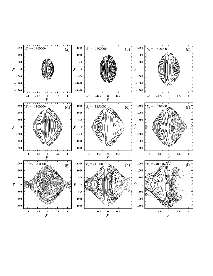
Figure 14 gives the phase space structure at various values of the Jacobi constant for the system QR3 at t=20, via the 2D approximation. The central value of the potential (potential well) and the value of the Jacobi constant at the Lagrangian points , are and respectively. The panels of the two upper rows of Fig.14 show the phase space structure for Jacobi constants below the value corresponding to (Note that the phase space areas corresponding to inside and outside corotation are divided). It is obvious that chaos becomes dominant for . The areas inside corotation with correspond to retrograde orbits of the ‘x4’ type (and their quasi-periodic orbits), while the areas with are filled with ‘x1’ orbits and their bifurcations.
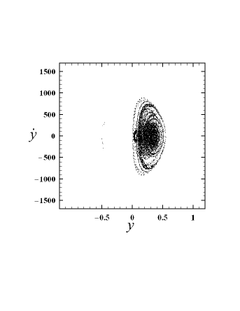
Figure 15 shows the projections of the real -body particles with energies on the SOS. The orbit of each real particle is integrated for 200 iterations. A distribution of the particles on layers corresponding to a foliation of invariant tori is discerned in this figure, despite the projection effects caused by the fact that the SOS is actually 4D. The central energy value is the same as in Fig.14c. At this value of the Jacobi constant there are almost no chaotic orbits inside corotation. Therefore, the orbits of Fig.15 are regular orbits close to the 2:1 and 3:1 resonances. Note that the area with , corresponding to orbits around the ‘x1’ periodic orbit, is well populated, while the area with corresponding to the ‘x4’ retrograde type of orbits is nearly devoid of real particles.
Figure 16 shows the energy (Jacobi constant) distribution of the real -body particles for the regular orbits (solid lines), and for the chaotic orbits (dashed lines) for the experiment QR3 at (gray) and (black). From Figs.14 and 16 we conclude that most chaotic orbits, with , are located outside corotation (the chaos is negligible inside corotation). On the other hand, for values greater than the above threshold there are chaotic orbits found both outside and inside corotation (mostly at the outer regions of the bar). In the 2D approximation, the chaotic orbits with energies which are located inside corotation, (Fig.14) are surrounded by invariant curves and, consequently, they cannot communicate with the regions outside corotation. The important remark is that the above result remains essentially valid for the orbits in the full 3D potential. Namely, the majority of the real chaotic orbits of the same energy levels which are located inside corotation remain there at least up to the end of our numerical integration, i.e. for times much longer than a Hubble time, although in the full 3D potential these orbits are in principle able to escape via the phenomenon of ‘Arnold diffusion’ (Arnold 1964).
We have found that of the particles in chaotic orbits of this experiment are located inside corotation and close to the end of the bar, therefore contributing to the backbone of the bar. The percentages of the particles in chaotic orbits which remain inside corotation, are shown in Table 1, for all the experiments. From this we conclude that this ‘chaotic component’ represents an important percentage of particles in all the experiments. The value of the Specific Finite Time Lyapunov Characteristic Number of these orbits is in general smaller than the value of of the chaotic orbits outside corotation. This can be inferred from Fig.17, in which the values of the orbits are plotted as functions of their values. The chaotic orbits have (see Voglis et al., 2006a). The regular orbits are almost completely located inside corotation (around the resonances 2:1 and 3:1) and have the smallest values of . The chaotic orbits, on the other hand, are spread in the whole range of resonances, but it is obvious that the most weakly chaotic orbits (having smaller ) are located inside corotation and therefore support the bar.
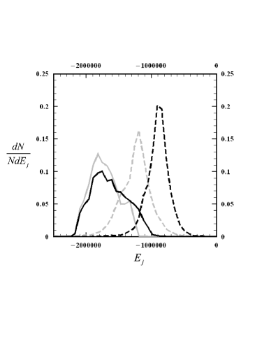
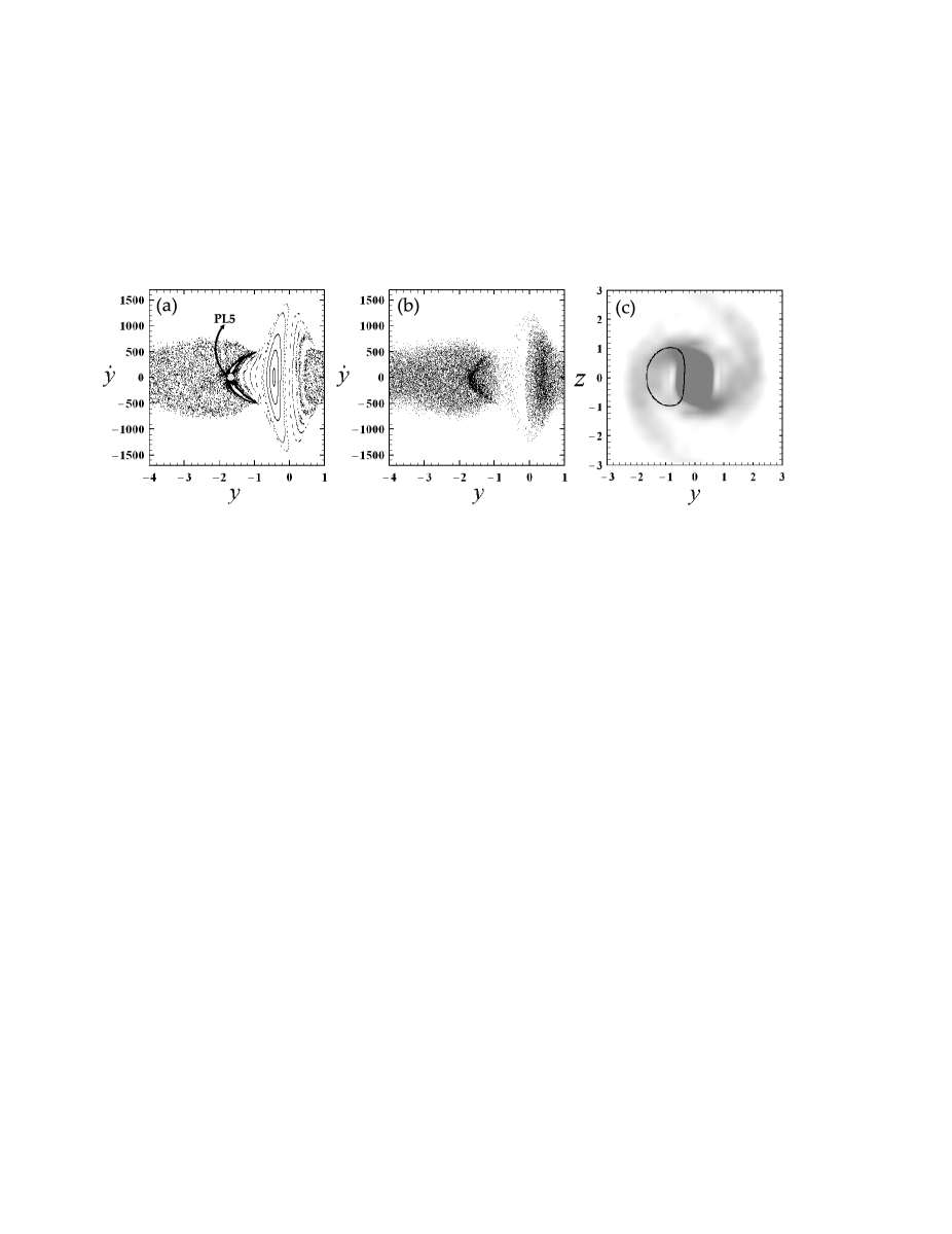
Figure 18a shows another SOS, obtained from the 2D approximation, for the experiment QR3 at and for the Jacobi constant . In this figure we see also the area outside corotation (which is located at ). A sticky region is apparent here between corotation and . This stickiness phenomenon is related to the unstable manifolds emanating from unstable periodic points with fixed points in the same area. This phenomenon, called ‘stickiness in chaos’ has been studied thoroughly in simple dynamical systems (see Contopoulos & Harsoula, 2008, and references therein). The corresponding Jacobi constant is the maximum of the energy distribution of the chaotic particles having the same angular velocity as the pattern speed of the bar (). The two stable periodic orbits located inside the sticky zone correspond to bifurcations of the main orbit around the point (named ‘PL5’) which has become unstable at this value of Jacobi constant. All the unstable asymptotic curves are necessarily parallel to the asymptotic curve of the simplest periodic orbit i.e. the short period orbit around . Thus this orbit is called ‘PL5’. In Fig.18b we plot the projection on the same SOS of the real particles. We observe again the depopulation of the ‘x4’ area and the ‘sticky’ region just outside corotation around the unstable ‘PL5’ orbit. Such ‘stickiness’ is observed in many energy levels and it is responsible for supporting various features of the system (QR3 at ). In Fig.18c we see the unstable periodic orbit (black), starting at the point ‘PL5’ of Fig.18a, superimposed to the backbone of the system QR3 at (gray). The ‘sticky’ behaviour of some orbits around the unstable ‘PL5’ orbit supports the ring type shape.
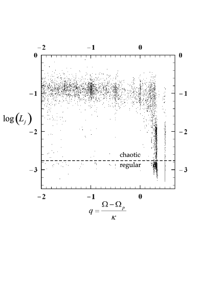
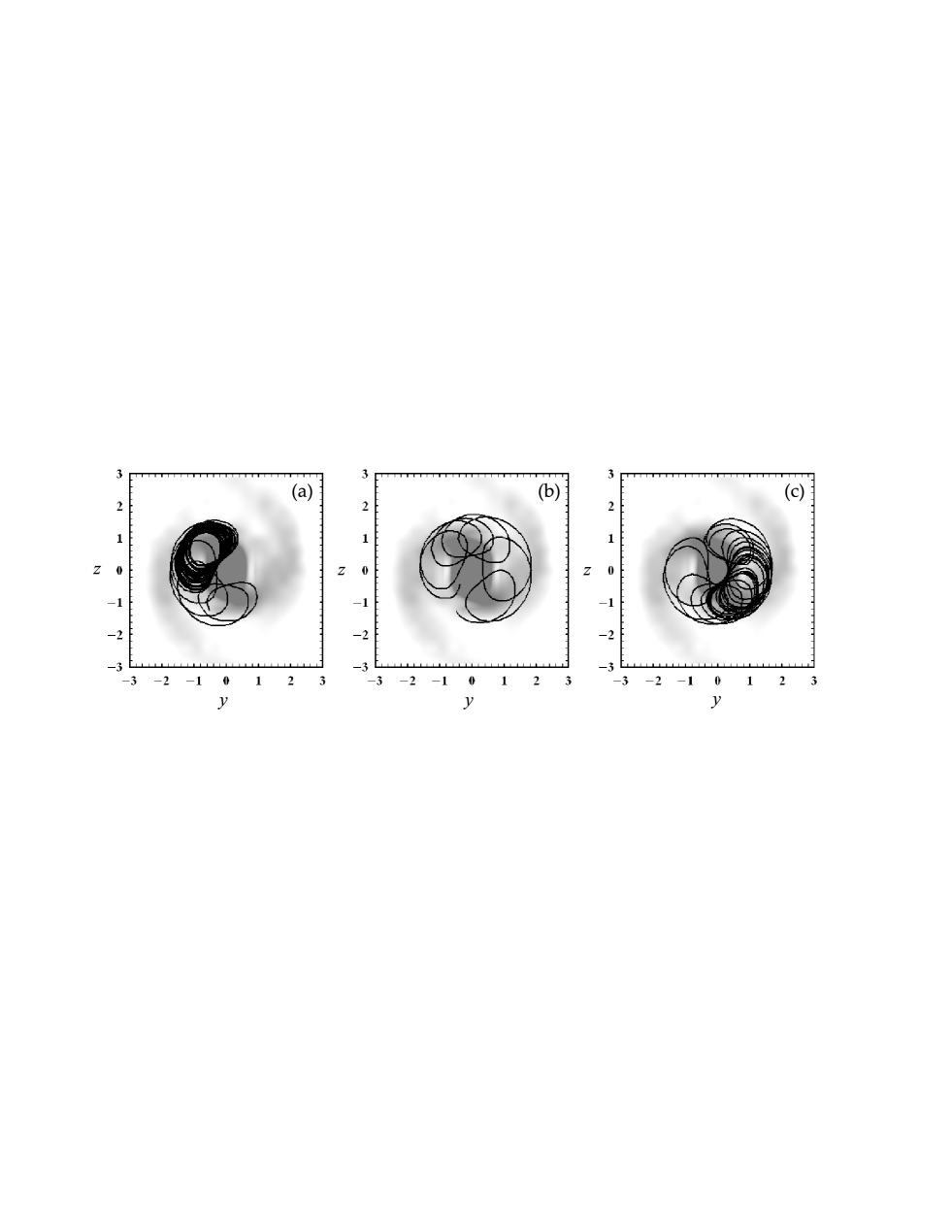
Figure 19 shows the evolution of a real chaotic orbit which presents ‘stickiness’ around the unstable ‘PL5’ orbit of Fig.18a. The calculated frequency of this orbit is , i.e. it has the same angular velocity as the bar and it forms precessing ‘bananas’. Such orbits amplify the formation of the ring, which can be classified as R1, as it is perpendicular to the bar (see Romero-Gomez et al., 2006).
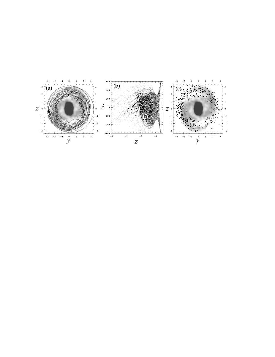
In Fig.20 we present the evolution of a real particle in chaotic orbit, of the experiment QR4 at , in the configuration space (Fig.20a) as well as in the phase space () (Fig.20b). This orbit has and (this Jacobi constant lies between and ). We see that the orbit on the configuration space is located outside corotation, filling the area all along the spiral arms (Fig.20a). In Fig.20b the SOS () is presented for 50 iterations of test particles, for , only for the area outside corotation. The integration time corresponds to 1.5-2.0 Hubble times. The ‘stickiness’ along the asymptotic curves of the periodic orbits is evident. In this value of the Jacobi constant the main unstable periodic orbit is the short period orbit ‘PL1’ or ‘PL2’, around the Lagrangian points and . We note that the density of points drops abruptly outside the radius that corresponds approximately to the end of the spiral arms. As there are no islands of stability or obvious cantori, the only possible reason of stickiness could be the trapping along the asymptotic curves of the unstable orbits. In Fig.20b the projections of 350 iterations of the real 3D chaotic orbit (black dots), are superimposed. We notice that these sections stay located inside the radius of the spiral arms. In general, the stickiness of the chaotic orbits along the asymptotic curves of the unstable curves of the short period orbit ‘PL1’ or ‘PL2’ as well as all the other curves from unstable periodic orbits of greater multiplicity, is responsible for the support of features like rings and spiral arms. In particular, the invariant manifolds from all the unstable periodic orbits (for values of between and ) cannot intersect each other. Thus they are forced to follow nearly parallel paths in the phase space, and this enhances the structures supported by them, i.e. the rings and the spiral arms. A thorough study of the role of asymptotic curves in the maintenance of spiral structure is done in Voglis et al. (2006b) and Tsoutsis et al. (2008). They showed that the apocentres of all the chaotic orbits with initial conditions along the manifolds corresponding to the unstable periodic orbits with Jacobi constants create an invariant locus supporting the spiral arms. In Fig.20c we plot only the apocentres of the orbit plotted in Fig.20a (black dots in Fig.20c), where we observe that they coincide very well with the outer parts of the ring and with the spiral arms (gray background).
4 CONCLUSIONS
We present a detailed investigation of the orbital structure of four different -body experiments simulating barred-spiral galaxies exhibiting significant secular evolution within one Hubble time. The study has been made for two different snapshots during the evolution of the systems, an early snapshot (t=20) and a late one in which the systems are close to equilibrium (t=300). The amplitude of the bar is large in all the experiments and the spin parameter has a value close to the one of our Galaxy.
The main conclusions of our study are the following:
(i) The ellipticity profile of the bar’s isophotes evolves from flat, at t=20, to declining at t=300, when the systems are close to equilibrium.
(ii) The boxiness of the bar’s isophotes and the pattern speed () of the bar are correlated, i.e the boxiness decreases with increasing .
(iii) Using frequency analysis we have found the main resonances around which the -body particles in regular orbits are concentrated. The particles in the chaotic orbits are more scattered in their frequency maps, however we can still detect concentrations around a variety of resonances, larger than in the case of the particles in regular orbits.
(iv) Almost the whole mass component in regular orbits are particles located inside corotation. These particles support the bar. The most populated type of resonant regular orbit is the 2:1 or ‘x1’ type of orbit. Another important group of regular orbits corresponds to the 3:1 resonance at t=20 (except from the experiment QR1). This gradually transforms to a group ‘A’ type of orbit at t=300. Group ‘A’ is responsible for the boxiness of the bar’s isophotes.
(v) Group ‘B’ corresponds to retrograde ‘x4’ type of orbits and exhibits a very small component both in regular and chaotic orbits, which becomes almost negligible in experiments with great values of the bar’s pattern speed .
(vi) Chaotic orbits exist only beyond a threshold of values of the Jacobi constant value . An important percentage of them are located inside corotation near the resonances 2:1, 3:1, 4:1 and the group ‘A’ and support the outer regions of the bar. This component of the chaotic population has the smallest values of the Specific Finite Time Lyapunov Characteristic Number among all the chaotic orbits. Therefore, these orbits can be considered as weakly chaotic, resembling to regular orbits even when they are integrated for times much longer than a Hubble time.
(vii) Comparing 2D surfaces of sections for test particles with projections on the same surfaces of sections for real -body particles we conclude that the areas corresponding to the ‘x4’ type of orbits are depopulated. The chaotic domain in the surface of section, inside corotation, are limited by invariant curves in the 2D approximation of test particles. The same seems to be true for the projections on the surface of section of the real -body chaotic orbits, despite the third dimension.
(viii) There are chaotic domains in the surface of section, just outside corotation, that show ‘stickiness’ due to the existence of asymptotic manifolds of some unstable periodic orbits. The stickiness is observed in both the test particles and the real -body particles. These domains correspond to chaotic orbits that present a very slow diffusion before escaping from their systems, and therefore they are responsible for the maintenance of the general features of the systems such as rings and spiral arms.
(ix) The corresponding frequencies responsible for the formation of the ‘R1’ rings around the bar, in all our experiments have values around and , while the chaotic orbits that are responsible for the spiral arms have frequencies .
Acknowledgments
We would like to thank professor G. Contopoulos and Dr. C. Efthymiopoulos for useful discussions and for a careful reading of the manuscript with many suggestions for improvement. Finally, we would like to thank the referee for his useful remarks that helped us to improve our paper.
References
- Allen et al. (1990) Allen A.J., Palmer P.L., Papaloizou J., 1990, MNRAS, 242, 576.
- (2) Aquilano R.O., Muzzio J.C., Navone H.D., Zorzi A.F., 2007, CeMDA, 99, 307.
- Arnold (1964) Arnold V.I., 1964, Sov. Math. Dokl., 6, 581.
- Athanassoula et al. (1983) Athanassoula E., Byenayme O., Martinet L., Pfenniger D., 1983, A&A, 127, 349.
- Athanassoula et al. (1990) Athanassoula E., Morin S., Wozniak H., Puy D., Pierce M., Lombard J., Bosma A., 1990, MNRAS, 245, 130.
- Athanassoula (2003) Athanassoula E., 2003, MNRAS, 341, 1179.
- Athanassoula et al. (2008) Athanassoula E., Romero-Gomez M., Masdemont J.J., 2008, MNRAS, (in press).
- Barnes and Tohline (2001) Barnes E., Tohline E., 2001, ApJ, 551, 80.
- Berentzen et al. (2001) Berentzen I, Shlosman I. and Jogee S., 2006, ApJ, 637, 582.
- Binney and Spergel (1982) Binney J., Spergel D., 1982, ApJ, 252, 308.
- Ceverino & Klypin (2007) Ceverino D., Klypin A., 2007, MNRAS, 379, 1087.
- Contopoulos & Mertzanides (1977) Contopoulos G., Mertzanides C., 1977, A&A, 61, 477.
- Contopoulos (1979) Contopoulos G., 1979, A&A, 71, 221.
- Contopoulos & Papayannopoulos (1980) Contopoulos G., Papayannopoulos T., 1980, A&A, 92, 33.
- Contopoulos & Grosbol (1989) Contopoulos G., Grosbol P., 1989, A&AR, 1, 261.
- Contopoulos (2002) Contopoulos G., 2002, ”Order and Chaos in Dynamical Astronomy”, Springer-Verlag, Berlin.
- Contopoulos & Patsis (2006) Contopoulos G., Patsis P.A., 2006, MNRAS, 369, 1039.
- Contopoulos & Harsoula (2008) Contopoulos G., Harsoula M., 2008, Int. J. Bif. Chaos, 18, 2929.
- Efstathiou & Jones (1979) Efstathiou G., Jones B.J.T., 1979, MNRAS, 186, 133.
- Gonzalez-Garcia et al. (2006) Gonzalez-Garcia A.C., Barcells M., Olsevsky V.S., 2006, MNRAS, 372, L78.
- Holley-Bockelmann et al. (2001) Holley-Bockelmann K., Mihos J.C., Sigurdsson S., Hernquist L., 2001, ApJ, 549, 862.
- Holley-Bockelmann et al. (2002) Holley-Bockelmann K., Mihos J.C., Sigurdsson S., Hernquist L., Norman C.: 2002, ApJ, 567, 817.
- Kalapotharakos & Voglis (2005) Kalapotharakos C. and Voglis N.: 2005, Cel. Mech. Dyn. Astron., 92, 157.
- Kaufmann & Contopoulos (1996) Kaufmann D.E., Cotnopoulos G., 1996, A&A, 309, 381.
- Kaufmann & Patsis (2005) Kaufmann D.E., Patsis P.A., 2005, ApJ, 624, 693.
- Laskar (1990) Laskar J., 1990, Icarus, 88, 266.
- Lynden-Bell & Kalnajs (1972) Lynden-Bell D., Kalnajs A.J., 1972, MNRAS, 157, 1.
- Martinez-Valpuesta et al. (2006) Martinez-Valpuesta I., Shlosman I., Heller C., 2006, ApJ, 637, 214.
- Muzzio (2006) Muzzio J.C., 2006, Cel. Mech. Dyn. Astron., 96, 85.
- Naab et al. (1999) Naab T., Burkert A., Hernquist L., 1999, ApJ, 523, 133.
- Papaphilipou & Laskar (1996) Papaphilipou Y., Laskar J., 1996, A&A, 307, 427.
- Papaphilipou & Laskar (1998) Papaphilipou Y., Laskar J., 1998, A&A, 329, 451.
- Papayannopoulos & Petrou (1983) Papayannopoulos T., Petrou M., 1983, A&A, 119, 21.
- Patsis et al. (1997) Patsis P.A., Athanassoula E., Quillen A.C., 1997, ApJ, 483, 731.
- Patsis et al. (2002a) Patsis P.A., Skokos Ch., Athanassoula E., 2002a, MNRAS, 333, 847.
- Patsis et al. (2002b) Patsis P.A., Skokos Ch., Athanassoula E., 2002b, MNRAS, 333, 861.
- Patsis et al. (2002c) Patsis P.A., Skokos Ch., Athanassoula E., 2002c, MNRAS, 337, 578.
- Patsis et al. (2003a) Patsis P.A., Skokos Ch., Athanassoula E., 2003, MNRAS, 342, 69.
- Patsis et al. (2003b) Patsis P.A., Skokos Ch., Athanassoula E., 2003, MNRAS, 346, 1031.
- Patsis (2006) Patsis P.A., 2006, MNRAS, 369, 56.
- Peebles (1969) Peebles P.J.E., 1969, ApJ, 155, 393.
- Pfenniger (1984) Pfenniger D.,: 1984, A&A, 134, 373.
- Pfenniger & Friedli (1991) Pfenniger D., Friedli D., 1991, A&A, 252, 75.
- Quillen (2003) Quillen A.C., 2003, Astron. J., 125, 785.
- Romero-Gomez et al. (2006) Romero-Gomez M., Masdemont J.J., Athanassoula E., Garcia-Gomez C., 2006, A&A, 453, 39.
- Romero-Gomez et al. (2007) Romero-Gomez M., Athanassoula E., Masdemont J.J., Garcia-Gomez C., 2007, A&A, 472, 63.
- Shen & Sellwood (2004) Shen J., Sellwood A., 2004, ApJ, 604, 614.
- Sidlichovsky & Nesvorny (1997) Sidlichovsky M., Nesvorny D., 1996, Cel. Mech. Dyn. Astron., 65, 137.
- Skokos (2001) Skokos Ch., 2001, J. Phys. A: Math.Gen., 34, 10029.
- Skokos (2002) Skokos Ch., Patsis, P.A. and Athanassoula E., 2002, MNRAS, 333, 847.
- Sparke & Sellwood (1987) Sparke L., Sellwood J.A., 1987, MNRAS, 225, 653.
- Sundin et al. (1993) Sundin M., Donner K.J., Sundelius B., 1993, A&A, 280, 105.
- Sundin (1996) Sundin M.: 1996, “Barred Galaxies”, ASP Conference Series, eds. Buta R., Crocker D.A. and Elmegreen B.G., 921 p.423.
- Teuben & Sanders (1985) Teuben P.J., Sanders R.H., 1985, MNRAS, 212, 257
- Tremaine & Weinberg (1984) Tremaine S., Weinberg M., 1984, MNRAS, 209, 729.
- Tsoutsis et al. (2008) Tsoutsis P., Efthymiopoulos C., Voglis N., 2008, MNRAS, 387, 1264.
- Voglis et al. (2002) Voglis N., Kalapotharakos C., Stavropoulos I., 2002, MNRAS, 337, 619.
- Voglis et al. (2006a) Voglis N., Stavropoulos I., Kalapotharakos C., 2006a, MNRAS, 372, 901.
- Voglis et al. (2006b) Voglis N., Tsoutsis P., Efthymiopoulos C., 2006b, MNRAS, 373, 280.
- Voglis et al. (2007) Voglis N., Harsoula M., Contopoulos G., 2007, (Paper I), MNRAS, 381, 757.
- Weinberg (1985) Weinberg M., 1985, MNRAS, 213, 451.