Analytic Theory of Edge Modes in Topological Insulators

Abstract

Spectrum and wave function of gapless edge modes are derived analytically for a tight-binding model of topological insulators on square lattice. Particular attention is paid to dependence on edge geometries such as the straight (1,0) and zigzag (1,1) edges in the thermodynamic limit. The key technique is to identify operators that combine to annihilate the edge state in the effective one-dimensional (1D) model with momentum along the edge. In the (1,0) edge, the edge mode is present either around the center of 1D Brillouin zone or its boundary, depending on location of the bulk excitation gap. In the (1,1) edge, the edge mode is always present both at the center and near the boundary. Depending on system parameters, however, the mode is absent in the middle of the Brillouin zone. In this case the binding energy of the edge mode near the boundary is extremely small; about $10^{-3}$ of the overall energy scale. Origin of this minute energy scale is discussed.

1 Introduction

Recently, a new class of topological insulator (TI), also referred to as quantum spin Hall (QSH) insulator, has been attracting much interest in both theory [1, 2, 3, 4, 5, 6, 7] and experiments [8, 9, 10]. Different from conventional insulators, QSH insulators have topologically protected helical edge states with the spectrum lying in the bulk insulating gap.[1, 12, 13] Two-dimensinal (2D) topological insulator has been realized in HgTe/CdTe quantum wells[8] following theoretical suggestion of Bernevig, Hughes and Zhang[6] who proposed a useful model, hereafter referred to as the BHZ Model. Helical edge state has been further studied using the resultant continuum model.[14, 15] The BHZ model is not realistic away from the zone center, since it is based on the $\mib k\cdot\mib p$ perturbation theory and envelope-function approximation. However, a regularization of the model using the tight-binding scheme has the simple structure for the whole Brillouin zone (BZ), and is suitable for studying the general property of QSH systems. Note that characterization of the topological property of the system requires information of wave functions over the whole BZ.

In this paper, we derive the spectrum of edge modes analytically taking the tight-binding version of the BHZ model for the square lattice. In contrast to previous study of edge modes,[11, 14] we take not only the straight (1,0) edge but also the zigzag (1,1) edge, and make detailed comparison of respective edge modes. This comparison is partially inspired by the remarkable difference between the zigzag and armchair edges in graphene [16, 17]. In contrast to the latter, however, the edges in the present model should not be taken as representing the HgTe/CdTe quantum wells since the short-distance behavior of the model is not realistic. Nevertheless, the intuition gained by the exact solution of the simplified model should provide useful information for understanding more complicated systems.

In a separate paper[18], we have already derived the spectrum of both straight and zigzag edges relying partially on numerical method. In particular, we have found for the zigzag edge a reentrant mode with tiny binding energy. Since the relevant energy is so small as compared with the overall energy, it is desirable to characterize its nature analytically. Then the origin of tiny binding energy should be clarified. In the present paper, we derive fully analytic expressions of not only the spectrum for both edges, but also momentum regions allowed for the modes. Namely we derive critical momentum where the edge mode merges with bulk excitations. Our analytical method is a systematic generalization of previous ones [19, 11] so that the spectrum can be obtained for general direction of the edge.

This paper is organized as follows: In §2, we review the lattice version of the BHZ model with nearest-neighbor transfer, paying attention to its symmetry property in the 2D BZ. Sections 3 and 4 are devoted to analytic derivation of edge modes for straight and zigzag edges, respectively. We use a systematic method to derive the spectrum in terms of the “annihilator”. Existent regions of edge modes are derived for both straight and zigzag edges. In the zigzag case, we find a novel reentrant edge mode with a tiny binding energy below the bulk spectrum. Finally, we summarize the results and discuss their implication in Sec. 5.

2 Model with particle-hole symmetry

We consider the BHZ model given by the following $4\times 4$ matrix:

$$H(\mib k)=\left[\begin{array}[]{cc}h(\mib k)&0\\ 0&h^{*}(-\mib k)\\ \end{array}\right],$$ (3)

where $\mib k=(k_{x},k_{y})$ is a 2D crystal momentum, measured from $\Gamma$-point. The lower-right block $h^{*}(-\mib k)$ is a $2\times 2$ matrix, and is deduced from the upper-left block $h(\mib k)$ by time reversal transformation. $h(\mib k)$ is parametrized as,

$$h(\mib k)=\mib d(\mib k)\cdot\mib\sigma=\left[\begin{array}[]{cc}d_{z}&d_{x}-id_{y}\\ d_{x}+id_{y}&-d_{z}\end{array}\right],$$ (4)

where $d_{i}(\mib k)$ are given by

$$d_{x}({\mib k})=A\sin k_{x},\quad d_{y}({\mib k})=A\sin k_{y},$$ (5)

$$d_{z}({\mib k})=\Delta-2B(2-\cos k_{x}-\cos k_{y}),$$ (6)

with the lattice constant $a$ set to unity[6]. We only consider the case $A>0,\ B>0$ and $\Delta\geq 0$ in this paper. The same signs of $B$ and $\Delta$ are necessary for topological insulator. The solution for $A<0$ is trivially obtained from that for $H(-\mib k)$. Each row and column of eq. (4) represent spin-orbital states associated with the $s$-type $\Gamma_{6}$ and the $p$-type $\Gamma_{8}$ orbitals of the 3D band structure of HgTe and CdTe. Other parameters which appear in Ref.BHZ, i.e., $C$ and $D$ have been set to zero. As a result, the spectrum has the particle-hole symmetry that simplifies the analysis.

The $2\times 2$-matrix Hamiltonian $h(\mib k)$ is equivalent to the following tight-binding Hamiltonian on the square lattice:

$$h_{\uparrow} =\sum_{I,J}c_{I,J}^{\dagger}\hat{\cal E}c_{I,J}$$

$$+\left(c_{I,J}^{\dagger}\hat{t}_{x}c_{I+1,J}+c_{I,J}^{\dagger}\hat{t}_{y}c_{I,J+1}+h.c.\right),$$ (7)

where we have introduced for each site $(I,J)$ the two-component field:

$$c^{\dagger}=(c^{\dagger}_{s\uparrow},c^{\dagger}_{p\uparrow})$$ (8)

with orbitals $s,p$. The tight-binding parameters are given by

$$\hat{\cal E} =(\Delta-4B)\sigma_{z},$$ (9)

$$\hat{t}_{x} =-i{A\over 2}\sigma_{x}+B\sigma_{z},$$ (10)

$$\hat{t}_{y} =-i{A\over 2}\sigma_{y}+B\sigma_{z},$$ (11)

each of which is a $2\times 2$ matrix. The down spin part $h_{\downarrow}$ corresponding to the lower-right block of eq.(3) is obtained by replacing $\hat{t}_{i}$ with its complex conjugation $\hat{t}_{i}^{*}$.

We consider the BHZ model over the whole BZ of the square lattice. Bulk energy $E_{\rm b}({\mib k})$ is written as

$$E_{\rm b}({\mib k}) =\pm\left\{A^{2}\left(\sin^{2}k_{x}+\sin^{2}k_{y}\right)\right.$$

$$+\left.\left[\Delta-4B+2B\left(\cos k_{x}+\cos k_{y}\right)\right]^{2}\right\}^{1/2},$$ (12)

which is symmetric with respect to positive (conduction) and negative (valence) energy bands, being the signature of the particle-hole symmetry. As one varies mass parameter $\Delta$, there appear four gap closing points, namely at $\Gamma=(0,0)$, $X=(\pi,0)$, $X^{\prime}=(0,\pi)$ and $M=(\pi,\pi)$. Note that these points are invariant against time-reversal operation. Gap closing at $\Gamma$ occurs when $\Delta=0$, whereas the gap closing at $X$ and $X^{\prime}$ occurs simultaneously when $\Delta=4B$, at $M$ when $\Delta=8B$.

3 Straight edge

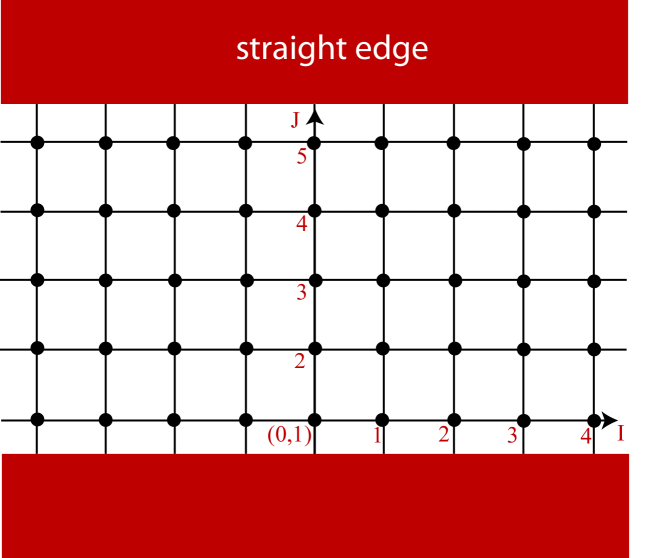
Figure 1: Straight edge lattice ribbon with two boundaries in (1,0) direction.

3.1 Effective one-dimensional form

Let us first consider the geometry (see Fig. 1), in which electrons are confined to $N_{r}$ rows in a strip between $y=1$ and $y=N_{r}$, i.e., the two edges are along $x$-axis. Translational invariance along $x$-axis allows for constructing a 1D Bloch state with a crystal momentum $k=k_{x}$:

$$|k,J\rangle=\frac{1}{\sqrt{N_{c}}}\sum_{I}e^{ikI}|I,J\rangle,$$ (13)

where $I,J$ represents lattice site, $N_{c}$ is the number of sites along the $x$-axis, and $|I,J\rangle=c_{I,J}^{\dagger}|0\rangle$. In order to introduce the edges, it is convenient to rewrite eq. (7) in form of a hopping Hamiltonian between neighboring rows. In terms of the two-component creation and annihilation operators $c^{\dagger}_{J}(k)$ and $c_{J}(k)$ associated with Bloch state (13), one can rewrite eq. (7) as

$$h_{\uparrow} =\sum_{k}h_{01}(k),$$ (14)

$$h_{01}(k) =\sum_{J}c^{\dagger}_{J}(k)\hat{\cal E}(k)c_{J}(k)$$

$$+\sum_{J}\left[c^{\dagger}_{J}(k)\hat{t}_{y}c_{J+1}(k)+h.c.\right]$$ (15)

where $\hat{\cal E}(k)$ is given by

$$\hat{\cal E}(k)=A\sin k\sigma_{x}+\left(\Delta_{B}+2\cos k\right)\sigma_{z},$$ (16)

Here and in the following, we use the notation $\Delta_{B}\equiv\Delta-4B$, and take the energy unit so that $B=1$. The corresponding Schrödinger equation is given by

$$\hat{\cal E}(k)\Psi_{J}+\hat{t}_{y}\Psi_{J-1}+\hat{t}_{y}^{\dagger}\Psi_{J+1}=E_{\uparrow}(k)\Psi_{J}$$ (17)

where $\Psi_{J}$ is the two-component amplitude with row index $J$. The straight edges along the $J=1$ row and $J=N_{r}$ row can be implemented by open boundary condition $\Psi_{0}=\Psi_{N_{r}+1}=0$.

It has been shown [14] in the continuum approximation of eq.(17) that there appear modes, which are localized on both edges of the system, with the particle-hole symmetric spectrum and a minimum gap at $k=0$. The origin of the gap is the overlap of wave functions on different edges. As $N_{r}$ tends to infinity, the gap disappears since the overlap becomes zero. In this limit one can identify edge modes localized on either edge. In the thermodynamic limit, the spectrum $E(k)$ of an edge mode near $J=1$ becomes an odd function of $k$, and the other edge mode has the spectrum $-E(k)$. The continuum approximation of Ref.cm has a limited validity, but emergence of the zero mode at $k=0$ in the thermodynamic limit $N_{r}\rightarrow\infty$ is guaranteed by the time-reversal and particle-hole symmetries [19, 11]. In the following, we deal with the thermodynamic limit.

3.2 Separation into Hermitian and annihilating parts

Our strategy to obtain the edge spectrum is best illustrated in the straight edge. Although the spectrum in this case has already been obtained in the literature [19, 11], we here present our way of derivation that can be extended to the zigzag edge. We try an edge state solution with property: $\Psi_{J+1}=\lambda\Psi_{J}\equiv\lambda^{J+1}\Psi$ with $|\lambda|<1$[19, 20], and derive the vector $\Psi$. Then eq.(17) can be written in the following form:

$$\left[\hat{\cal E}(k)+\lambda\hat{t}_{y}^{\dagger}+\frac{1}{\lambda}\hat{t}_{y}\right]\Psi\equiv P_{01}(\lambda,k)\Psi=E_{\uparrow}(k)\Psi,$$ (18)

where $P_{01}(\lambda,k)$ can be rearranged as

$$P_{01}(\lambda,k)=\mib\gamma\cdot\mib\sigma,$$ (19)

with components

$$\gamma_{x} =A\sin k$$ (20)

$$\gamma_{y} =i\frac{A}{2}\left(\lambda-\lambda^{-1}\right)$$ (21)

$$\gamma_{z} =\left(\lambda+\lambda^{-1}\right)+\Delta_{B}+2\cos k$$ (22)

For a general complex vector $\mib\gamma$, the eigenvalues of $P_{01}$ are also complex. However, we obtain real energy $E_{\uparrow}(k)$ in eq.(18) if one of the following conditions is met:
(a) all components of $\mib\gamma$ are real (including zero);
(b) the nonzero complex components combine to give zero when acting on the edge state. Such combination of operators is referred to as annihilator.
The condition (a) is not relevant here, because we would then have two eigenvalues $\pm E_{\uparrow}(k)$ and corresponding two eigenfunctions for a given $k$. Actually we should have only one edge mode for $h_{\uparrow}(k)$. Hence we have to accept the condition (b), and separate $P_{01}$ into a Hermitian part that gives the spectrum by diagonalization, and the rest that makes up the annihilator.

From eq.(21) and (22), coefficients $\gamma_{y}$ and $\gamma_{z}$ are both real only if $|\lambda|=1$. On the other hand, due to time-reversal symmetry and particle-hole symmetry of the system, the eigenvalue $E_{\uparrow}(k)$ is an odd function of $k$ in the thermodynamic limit [11, 14]. Therefore, $\sigma_{y}$ and $\sigma_{z}$ must both belong to the annihilator, and the only component to be diagonalized is $\sigma_{x}$. The annihilator corresponds to either $\sigma_{y}+i\sigma_{z}$ or $\sigma_{y}-i\sigma_{z}$, depending on the eigenvalue $\pm 1$ of $\sigma_{x}$.

Accordingly, we decompose $P_{01}(\lambda,k)$ as

$$P_{01}(\lambda,k)=H_{01}+F_{01},$$ (23)

$$H_{01}=A\sin k\,\sigma_{x},$$ (24)

$$F_{01}=\gamma_{y}\sigma_{y}+\gamma_{z}\sigma_{z},$$ (25)

where $F_{01}$ should form the annihilator. Namely, we impose the relation $\gamma_{z}=si\gamma_{y}$, according to the eigenvalue $s=\pm 1$ of $\sigma_{x}$. The relation is equivalent to

$$(1+\frac{sA}{2})\lambda+(1-\frac{sA}{2})\lambda^{-1}+m_{k}=0,$$ (26)

where we have introduced the notation:

$$m_{k}=\Delta_{B}+2\cos k.$$ (27)

By solving eq.(26) with $A\neq 2$, we obtain

$$\lambda_{\pm}(s)=\frac{-m_{k}\pm\sqrt{m^{2}_{k}+A^{2}-4}}{2+sA},$$ (28)

with the relation

$$\lambda_{\pm}(-s)=1/\lambda_{\mp}(s).$$ (29)

Provided the eigenvalue equation

$$H_{01}\Psi =E_{\uparrow}(k)\Psi.$$ (30)

is satisfied, then equality $F_{01}\Psi=0$ follows with eq.(26). In this way the edge spectrum is simply derived as

$$E_{\uparrow}(k)=sA\sin k.$$ (31)

with the eigenstate written as

$$\Psi(s)=\begin{pmatrix}1\\ s\end{pmatrix}.$$ (32)

Note that only one of $s=\pm 1$ is relevant, as discussed below.

The boundary condition $\Psi_{J=0}=0$ requires the edge state to have the form

$$\Psi_{J}(s)=\left[\lambda_{+}(s)^{J}-\lambda_{-}(s)^{J}\right]\Psi(s),$$ (33)

apart from the normalization factor. Since the wave function should decay as $J$ increases, the edge state can only be realized with $|\lambda_{\pm}(s)|<1$. Because of the relation eq.(29), there is at most one $s$ for given $k$ that describes the edge mode with the spectrum eq.(31). Hence there is only one edge state per spin and per momentum.

In a similar manner, we obtain another edge mode for $h_{\downarrow}$. The corresponding energy $E_{\downarrow}(k)$ is given by

$$E_{\downarrow}(k)=E_{\uparrow}(-k)=-E_{\uparrow}(k),$$ (34)

where the first equality corresponds to the time-reversal symmetry. The particle-hole symmetry connecting the rightmost and leftmost sides with the same $k$ involves different spins. Note that the Kramers pair has the same $\lambda_{\pm}(s)$ for given $k$ and $-k$. In certain range of $k$, however, the edge modes do not exist. This problem is studied in detail in the next section.

3.3 Allowed momentum range for edge modes

A pair of gapless edge modes per edge are always present in the topological insulator phase (TI) that appears for $0<\Delta<8$, i.e., $|\Delta_{B}|<4$ in the BHZ model. However, the number of zero points of helical edge states should be an odd multiple of two, including the degeneracy, in the 1D BZ [12]. If the edge modes with the spectrum $E=\pm A\sin k$ were present for the whole BZ, the zero points amount to four (an even multiple of two) which violates the topological stability [21]. Hence the edge modes must merge into bulk excitations at finite $\kappa_{m}$, and degenerate zero points occur either at $k=0$ or $k=\pi$, but not at both. Note that $k=0$ and $k=\pi$ are two time reversal invariant momenta in 1D BZ.

With $\Delta_{B}=0$, the energy gap closes at X points $(\pi,0)$ and $(0,\pi)$ in the 2D BZ, as seen from eq.(12). Let us classify the case of $-4<\Delta_{B}<0$ as TI-1, and the case of $0<\Delta_{B}<4$ as TI-2. Figure 2 shows the spectrum of edge modes in the TI-1 (upper panel) and TI-2 (lower panel). In the TI-1, the edge modes intersect at $k=0$, whereas in TI-2 they meet at $k=\pi$. Also shown is approximate bulk spectrum in the system that is derived from $E_{\rm b}(k,k_{y})$ by fixing $k_{y}$ to $2\pi n/N_{r}$ with $n=1,\ldots,N_{r}$. Each curve for the bulk spectrum corresponds to integer $n$.

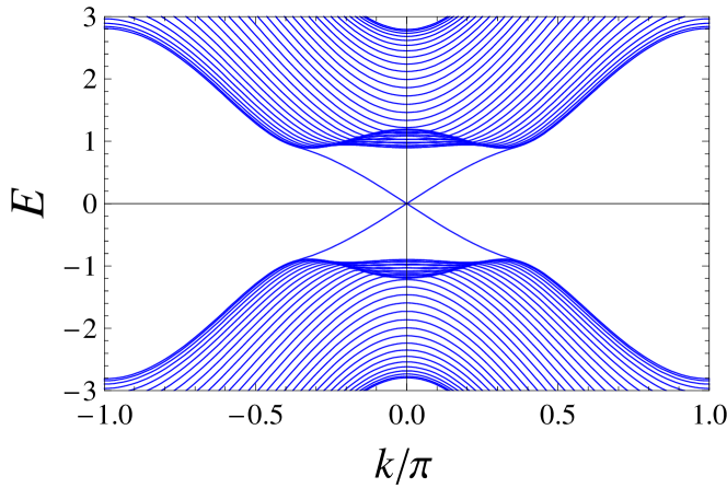
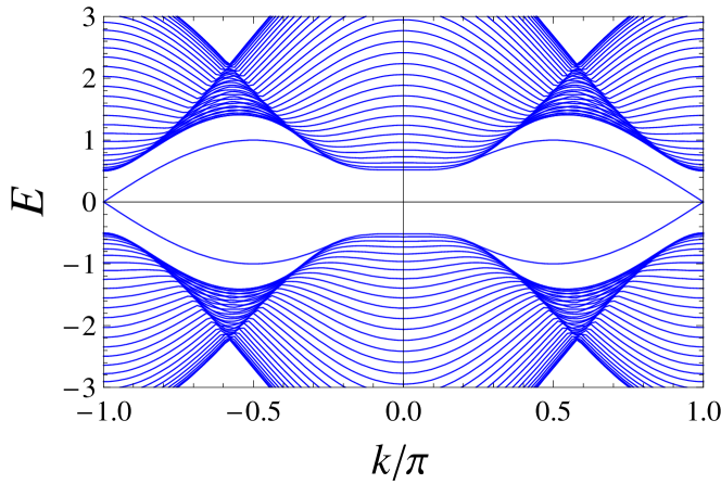
Figure 2: 1D energy bands in the straight edge: TI-1 (top) with $\Delta=1.2$ and TI-2 (bottom) with $\Delta=4.5$. In both cases, we set $A=1$. The edge modes have the spectrum $\pm A\sin k$ in the existent range of $k$.

We now derive the pair $\pm k_{m}$ of momentum where the edge mode merges with bulk excitations. In the following, we always assume $k\geq 0$ for simplicity. The merging occurs when the larger of $|\lambda_{\pm}(s)|$ becomes unity. Note that such $\lambda_{\pm}(s)$ is real, since otherwise $|\lambda_{\pm}(s)|$ is independent of $m_{k}$, and hence of $k$. For complex $\lambda_{\pm}(s)$ we obtain from eq.(28),

$$|\lambda_{\pm}(s)|^{2}=\frac{2-sA}{2+sA},$$ (35)

which is less than unity only with $s=1$. In this section we deal with the case $0<A<2$ that allows complex $\lambda_{\pm}(s)$. Then, edge modes are assured to be present for such $k$ with complex $\lambda_{\pm}(1)$, which is simply written as $\lambda_{\pm}$ hereafter. Edge modes in the case of $A>2$ will be discussed in §5.

TI-1 regime

In this case gapless points are present at $k=0$. Let us assume $m_{k}=\Delta_{B}+2\cos k<0$ when merging occurs at $k=k_{m1}$, Then we obtain $|\lambda_{+}|>|\lambda_{-}|$ for real $\lambda_{\pm}$, and the condition for merging is reduced to

$$\lambda_{+}=\frac{-m_{k}+\sqrt{m^{2}_{k}+A^{2}-4}}{2+A}=1.$$ (36)

from eq.(28). Then we obtain

$$\cos k_{m1}=1-\Delta/2,$$ (37)

which justifies the assumption $m_{k}<0$. One can check that there is no solution if we assume $m_{k}>0$. We note that eq.(37) has already been obtained by König et al.[11]

The condition for merging is also to have the same energy as the lowest bulk excitation for given $k$. The minimum of $E_{b}(k,k_{y})$ may occur either at $k_{y}=0$ or $k_{y}=\pm\arccos\left[2m_{k}/(A^{2}-4)\right]$ depending on the value of $k$. If the threshold of bulk excitations with $k=k_{m1}$ occurs at $k_{y}=0$, merging momentum $k_{m1}$ is simply obtained from eq.(12) as

$$\Delta_{B}+2+2\cos k=m_{k}+2=0,$$ (38)

which is consistent with eq.(37). Namely, the condition $\lambda_{+}=1$ is equivalent to having the same energy for edge mode and for the minimum of bulk excitations. Furthermore, it is easily seen that the group velocity $A\cos k_{m1}$ at merging point is common to both edge mode and the lowest bulk excitation. Namely, the edge mode vanishes at such $k$ that it has the common tangent with the threshold of bulk excitations $E_{b}(k,k_{y})$ with $k_{y}=0$.

The crossings of 1D energy bands in Fig.2 indicates the transition from the lowest bulk excitation $E_{b}(k,k_{y})$ with $k_{y}=0$ to with $k_{y}=\pm\arccos\left[2m_{k}/(A^{2}-4)\right]$. The critical momentum $k_{c1}$ satisfies the condition

$$\partial^{2}E_{\rm b}(k_{c1},k_{y})/\partial k_{y}^{2}|_{k_{y}=0}=0,$$ (39)

which gives the solution

$$\cos k_{c1}=1-\frac{\Delta}{2}+\frac{A^{2}}{4}.$$ (40)

The threshold has $k_{y}=0$ for $k>k_{c1}>0$. By comparing with eq.(37), we find $\cos k_{c1}>\cos k_{m1}$, which means $0\leq k_{c1}<k_{m1}$. Namely, merging with bulk excitations indeed occurs in the range where $k_{y}=0$ corresponds to the threshold.

TI-2 regime

In this case edge modes exist around $k=\pi$. Let us assume $m_{k}>0$ when merging occurs at $k=k_{m2}>0$. The condition for merging is now given by

$$\lambda_{-}=\frac{-m_{k}-\sqrt{m^{2}_{k}+A^{2}-4}}{2+A}=-1,$$ (41)

which gives $m_{k}=2$ as the solution, or

$$\cos k_{m2}=1-\Delta_{B}/2=3-\Delta/2.$$ (42)

In the TI-2 regime, the threshold of bulk excitations occurs at $k_{y}=\pi$ or $k_{y}=\pm\arccos\left[2m_{k}/(A^{2}-4)\right]$. It can be checked that the bulk energy at $\mib k=(k_{m2},\pi)$ becomes the same as the edge mode with the condition (42). Hence merging occurs with bulk excitations $E_{b}(k,k_{y})$ with $k_{y}=\pi$.

The critical momentum $k=k_{c2}$, below which the minimum of $E_{b}(k,k_{y})$ no longer occurs at $k_{y}=\pi$, can be obtained by condition

$$\partial^{2}E_{\rm b}(k_{c2},k_{y})/\partial k_{y}^{2}|_{k_{y}=\pi}=0,$$ (43)

which gives the solution

$$\cos k_{c2}=1-\frac{\Delta_{B}}{2}-\frac{A^{2}}{4}.$$ (44)

Thus we have the relation $\cos k_{c2}<\cos k_{2m}$, or $k_{c2}>k_{2m}$. Hence merging indeed occurs in the range where $k_{y}=\pi$ corresponds to the threshold. In this way, we have quantified important characteristics of the edge modes shown in Fig.2.

4 Zigzag edge

4.1 Effective one-dimensional form

Let us now consider a zigzag edge geometry, as illustrated in Fig.3.

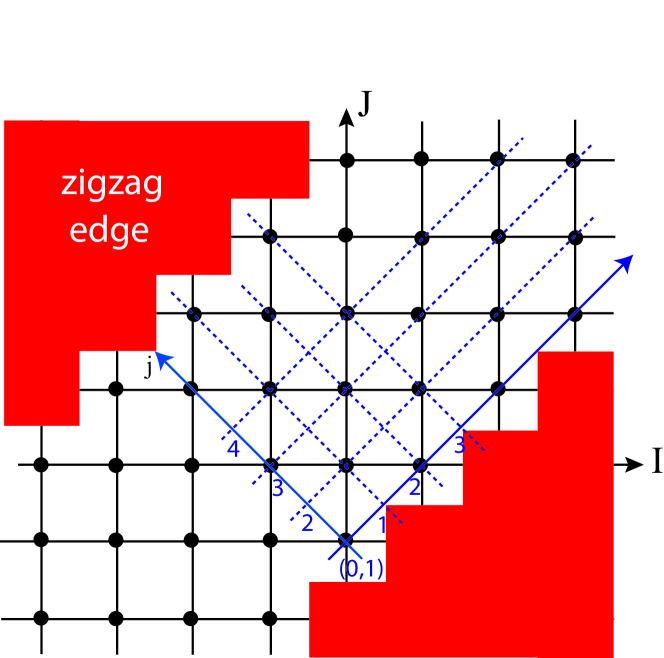
Figure 3: Zigzag edge lattice ribbon, with two boundaries in (1,1) direction.

Electrons in a zigzag edge geometry are confined in a diagonal strip: $1\leq y-x\leq N_{r}$, provided the edges are placed at $y-x=1$ and $y-x=N_{r}$, normal to the $(1,-1)$-direction. The translational invariance remains along the $(1,1)$-direction, where the conserved momentum is given by $p=(k_{x}+k_{y})/\sqrt{2}$. For notational convenience we introduce $\kappa=p/\sqrt{2}$ with ${-\pi/2<\kappa\leq\pi/2}$ and define the new basis set as

$$|\kappa,j\rangle=\frac{1}{\sqrt{N_{c}}}\sum_{I}\exp\left[i\kappa\left(2I+j\right)\right]|I,I+j\rangle,$$ (45)

where the site summation goes along the (1,1) direction. The phase factor is so chosen that it becomes unity for the state $|-\!J,J\rangle$. Then, the amplitude $\Phi_{j}$ in this basis satisfies the Schrödinger equation analogous to eq.(17):

$$\hat{\cal E}\Phi_{j}+\hat{t}_{11}(\kappa)\Phi_{j-1}+\hat{t}^{\dagger}_{11}(\kappa)\Phi_{j+1}=E_{\uparrow}(\kappa)\Phi_{j}$$ (46)

where $\hat{\cal E}$ has been defined by eq.(9) and hopping matrix $\hat{t}_{11}(\kappa)$ is given by

$$\hat{t}_{11}(\kappa) =\frac{i}{2}Ae^{-i\kappa}\sigma_{x}-\frac{i}{2}Ae^{i\kappa}\sigma_{y}+2\cos k\sigma_{z}$$ (47)

We impose the boundary condition: $\Phi_{0}=\Phi_{N_{r}+1}=0$, which is consistent with the zigzag edge geometry. Assuming eigenstate of eq.(46) with property $\Phi_{j}=\lambda\Phi_{j-1}=\lambda^{j}\Phi$, where $|\lambda|<1$,[19, 20] we obtain

$$\left(\hat{\cal E}+\lambda\hat{t}^{\dagger}_{11}(\kappa)+\lambda^{-1}\hat{t}_{11}(\kappa)\right)\Phi =P_{11}(\lambda,\kappa)\Phi=E_{\uparrow}(\kappa)\Phi$$ (48)

For later reference purpose, we write the bulk energy $E_{\rm b}$ in terms of variables $\kappa=(k_{x}+k_{y})/2$ and $\xi=(k_{x}-k_{y})/2$. From eq.(12) we obtain

$$E_{\rm b}(\kappa,\xi) =\pm\left[2A^{2}\left(\sin^{2}\kappa\cos^{2}\xi+\cos^{2}\kappa\sin^{2}\xi\right)\right.$$

$$+\left.\left(\Delta_{B}+4\cos\kappa\cos\xi\right)^{2}\right]^{1/2}.$$ (49)

4.2 Derivation of spectrum in thermodynamic limit

We will separate $P_{11}$ into the Hermitian part $H_{11}$ and the corresponding annihilator $F_{11}$. The separation now is not straightforward in contrast with the case of straight edge. As a preliminary, we introduce the following matrices:

$$\sigma_{X} =\left(\sigma_{x}+\sigma_{y}\right)/\sqrt{2},$$ (50)

$$\sigma_{Y} =\left(\sigma_{y}-\sigma_{x}\right)/\sqrt{2}.$$ (51)

Then we obtain

$$\hat{t}_{11}(\kappa)=\frac{A}{\sqrt{2}}\left(\sin{\kappa}\,\sigma_{X}-i\cos{\kappa}\,\sigma_{Y}\right)+2\cos{\kappa}\,\sigma_{z}.$$ (52)

We note that the spectrum of each edge mode is an odd function of $\kappa$. Then we introduce a variable $\theta$, which is an odd function of $\kappa$, and make the following transformation:

$$\sigma_{\theta x} ={\cos{\theta}}\,\sigma_{X}+{\sin{\theta}}\,\sigma_{z},$$ (53)

$$\sigma_{\theta z} ={\cos{\theta}}\,\sigma_{z}-{\sin{\theta}}\,\sigma_{X},$$ (54)

and rewrite as $\sigma_{\theta y}=\sigma_{Y}$. They keep the commutation property:

$$\left[\sigma_{\theta x},\sigma_{\theta y}\right]=2i\sigma_{\theta z},$$ (55)

and analogous cyclic ones that are the same as the original Pauli matrices. Then we obtain

$$\hat{\cal E} =\Delta_{B}\left(\sin{\theta\,}\sigma_{\theta x}+\cos{\theta\,}\sigma_{\theta z}\right),$$ (56)

$$\lambda\hat{t}^{\dagger}_{11}+\lambda^{-1}\hat{t}_{11} =\gamma_{\theta x}\sigma_{\theta x}+\gamma_{\theta y}\sigma_{\theta y}+\gamma_{\theta z}\sigma_{\theta z},$$ (57)

where

$$\gamma_{\theta x} =(\lambda+\lambda^{-1})\left(\frac{A}{\sqrt{2}}\sin{\kappa}\cos{\theta}+2\cos{\kappa}\sin{\theta}\right),$$ (58)

$$\gamma_{\theta y} =i(\lambda-\lambda^{-1})\frac{A}{\sqrt{2}}\cos{\kappa},$$ (59)

$$\gamma_{\theta z} =(\lambda+\lambda^{-1})\left(2\cos{\kappa}\cos{\theta}-\frac{A}{\sqrt{2}}\sin{\kappa}\sin{\theta}\right).$$ (60)

We choose $\Phi$ as eigenstate of $\sigma_{\theta x}$ since the coefficient $\Delta_{B}\sin\theta$ in eq.(56) is an odd function of $\kappa$. Then terms with $\sigma_{\theta y}$ and $\sigma_{\theta z}$ must combine to form the annihilator. Furthermore, since the coefficient of $\sigma_{\theta x}$ must be real, and be an odd function of $\kappa$, we require $\gamma_{\theta x}=0$. This condition determines $\theta$ in terms of $\kappa$ as

$$\sin{\theta} =-\frac{\tan{\kappa}}{\sqrt{\tan^{2}{\kappa}+8/A^{2}}},$$ (61)

$$\cos{\theta} =\frac{\sqrt{8}/A}{\sqrt{\tan^{2}{\kappa}+8/A^{2}}}.$$ (62)

In this way, we decompose $P_{11}=H_{11}+F_{11}$ in eq.(48) as follows:

$$H_{11} =\Delta_{B}\sin{\theta}\,\sigma_{\theta x},$$ (63)

$$F_{11} =(\Delta_{B}\cos{\theta}+\gamma_{\theta z})\sigma_{\theta z}+\gamma_{\theta y}\sigma_{\theta y}.$$ (64)

By diagonalizing $H_{11}$, the eigenenergy $E_{\uparrow}(\kappa)$ is derived as

$$E_{\uparrow}(\kappa)=s\Delta_{B}\sin{\theta},\quad(s=\pm 1),$$ (65)

where only one of the signs $\pm$ is relevant, as derived shortly. Note that the spectrum has a form analogous to the case of straight edge given by eq.(31). The condition for $F_{11}$ to form the annihilator is given by

$$\Delta_{B}\cos{\theta}+\gamma_{\theta z}=is\gamma_{\theta y}$$ (66)

which determines $\lambda$ for the edge mode as

$$\lambda_{\pm}(s)=\frac{1}{2\cos\kappa}\cdot\frac{-\Delta_{B}\cos{\theta}\pm\sqrt{R}}{2/\cos{\theta}+sA/\sqrt{2}},$$ (67)

with

$$R=\Delta_{B}^{2}\cos^{2}{\theta}-2\cos^{2}{\kappa}\left(8\cos^{-2}{\theta}-A^{2}\right).$$ (68)

In the case of $R<0$, we obtain complex $\lambda_{\pm}(s)$ with absolute value

$$|\lambda_{\pm}(s)|^{2}=\frac{\sqrt{8}-sA\cos{\theta}}{\sqrt{8}+sA\cos{\theta}},$$ (69)

which is less than unity only for $s=1$, and positive for $A^{2}\leq 8$. Therefore, the edge mode must have $s=1$ in eq.(65), and the group velocity is positive (negative) in TP-1 (TP-2) regime. A special case occurs with $\theta=\pm\pi/2$ that corresponds to $\kappa=\mp\pi/2$ according to eqs.(61) and (62). Actually eq.(67) gives $\lambda_{\pm}=\pm i$ at $\kappa=\pi/2$. Thus, at the boundary of the 1D BZ, there are no edge modes since $|\lambda_{\pm}|=1$. The neighborhood of this special point has $|\lambda_{\pm}|<1$, and there should be an edge mode. We emphasize that this property is independent of $\Delta$ and $A$, and is specific to the zigzag edge.

Due to the time-reversal symmetry, we obtain the Kramers partner from $h_{\downarrow}$ with the spectrum $E_{\downarrow}(\kappa)=-\Delta_{B}\sin{\theta}$. Figure 4 shows the edge modes together with bulk excitations for the TI-1 and TI-2, and the boundary case $\Delta_{B}=0$. The bulk spectrum illustrated is obtained from $E_{\rm b}(\kappa,\xi)$ as a function of $\kappa$ with fixed $\xi$. In both regimes, the edge mode becomes gapless at $\kappa=0$. Hence only $\kappa=0$ is the relevant point where a pair of edge modes are degenerate by time-reversal invariance. We note that the spectrum becomes completely flat with $\Delta_{B}=0$ [18].

In the low momentum region, the spectrum tends to the linear dispersion

$$E_{\uparrow,\downarrow}(\kappa)=\mp\frac{1}{\sqrt{8}}A\Delta_{B}\kappa=\mp\frac{1}{4}A\Delta_{B}p.$$ (70)

Especially, with $\Delta_{B}=\pm 4$, the spectrum becomes the same as the corresponding modes in the straight edge. Thus we find that the system acquires the axial symmetry only in the case of $\Delta_{B}=\pm 4$ even in the long-wavelength limit. This is not surprising since the difference in the edge shape remains even for long wavelength.

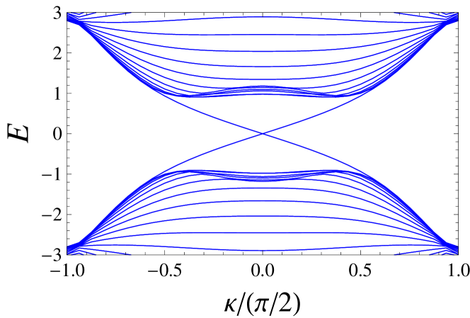
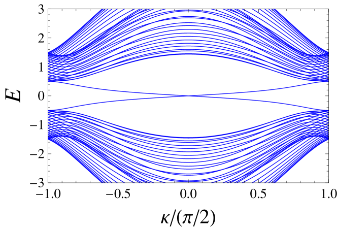
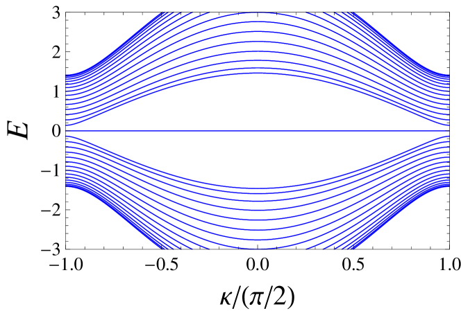
Figure 4: Spectrum of zigzag edge modes. The top panel is for TI-1 state with $\Delta=1.2$, the center is for TI-2 state with $\Delta=4.5$. The bottom panel shows the boundary case $\Delta=4$. All cases have $A=1$.

4.3 Allowed momentum range for edge modes

Let us first consider the edge mode in TI-1 regime corresponding to right-going edge mode (see Figure 2 top panel), and $\lambda_{\pm}=\lambda_{\pm}(1)$. We restrict to the region of positive $\kappa$. Since complex $\lambda$ always has a pair of solutions with $|\lambda_{\pm}|\leq 1$, the merging momentum $\kappa_{m}<\pi/2$ can be obtained from the condition

$$\lambda_{+}=1,$$ (71)

which is equivalent to

$$\left(8-A^{2}\right)\cos^{2}{\kappa_{m}}+2\Delta_{B}\cos{\kappa_{m}}+A^{2}=0,$$ (72)

according to eq.(67). Note that there is no solution for $0\leq\cos\kappa_{m}\leq 1$ in the case of $A^{2}\geq 8$. The relevant solution in the case of $A^{2}<8$ is given by

$$\cos{\kappa_{m}}=\frac{-\Delta_{B}\pm\sqrt{\Delta_{B}^{2}-A^{2}\left(8-A^{2}\right)}}{8-A^{2}},$$ (73)

The critical value of $\Delta_{B}$ beyond which no real $\kappa_{m}$ exists is given by

$$\Delta_{4c}=-A\sqrt{8-A^{2}}<0,$$ (74)

where we consider only the case $0<A<2$ as in the the straight edge. According to eq.(74), we have three cases:
(i) no solution for $\kappa_{m}<\pi/2$ with $\Delta_{B}>\Delta_{4c}$;
(ii) single $\kappa_{m}$ with $\Delta_{B}=\Delta_{4c}$;
(iii) two solutions $\kappa_{m1}<\kappa_{m2}$ with $\Delta_{B}<\Delta_{4c}$.
Edge modes in the case of $A>2$ will be discussed in §5.

The threshold of bulk excitations can occur either at $\xi=0$ or $\xi\neq 0$ depending on $\kappa$. The critical value $\kappa_{c}$ separating the two cases is determined by the condition

$$\partial^{2}E_{\rm b}(\kappa_{c},\xi)/\partial\xi^{2}|_{\xi=0}=0,$$ (75)

which can be reduced to

$$2(A^{2}-4)\cos^{2}\kappa_{c}-2\Delta_{B}\cos\kappa_{c}-A^{2}=0.$$ (76)

Then we obtain

$$\cos\kappa_{c}=\frac{\Delta_{B}\pm\sqrt{\Delta_{B}^{2}+2A^{2}(A^{2}-4)}}{2(A^{2}-4)}.$$ (77)

In the case of $\xi\neq 0$, the momentum $\xi$ at the threshold satisfy the condition

$$\cos\xi=\frac{-2\Delta_{B}\cos\kappa}{4+(4-A^{2})\cos 2\kappa}.$$ (78)

At the zone boundary $\kappa=\pi/2$, eq.(78) gives $\xi=\pm\pi/2$ as the solution. Here the edge mode has the energy $E_{\uparrow}(\pi/2)=-\Delta_{B}$, and the lowest bulk excitation has the same energy $E_{\rm b}(\pi/2,\pm\pi/2)=-\Delta_{B}$. Namely, $\kappa=\pi/2$ is always a merging point in the zigzag edge for any parameter settings.

In the following, we analyze the spectrum of the edge mode near the merging momentum according to classification (i), (ii), (iii) given above.

Edge modes for the whole BZ

Let us first consider the case (i): $\Delta_{B}>\Delta_{4c}$. With $A=1$, we obtain $\Delta_{4c}=-\sqrt{7}$, i.e., $\Delta_{c}\sim 1.354$ from eq.(74). Figure 5 shows $|\lambda_{\pm}|$ and the energy of the edge mode relative to the threshold of bulk excitations in this case with $\Delta=1.4$.

At the zone boundary, the edge mode merges with bulk excitations. The difference of energies is expanded as

$$E_{\uparrow}(\kappa)-E_{\rm b}(\kappa,\frac{\pi}{2})=\frac{A^{2}}{\Delta_{B}}(\kappa-\frac{\pi}{2})^{2}+O\left((\kappa-\frac{\pi}{2})^{4}\right).$$ (79)

Note that only even order terms appear in the expansion since both the lowest bulk excitation $E_{\rm b}$ and edge mode energy $E_{\uparrow}$ are symmetric around $\pi/2$.

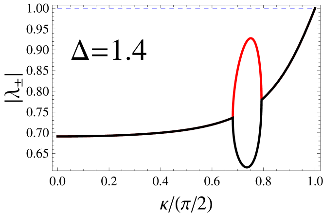
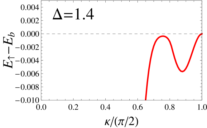
Figure 5: The parameter $|\lambda_{\pm}|$ and energy difference $E_{\uparrow}-E_{\rm b}$ between edge mode and the threshold of bulk excitations as a function of $\kappa$ for $\Delta=1.4$ with $A=1$. For complex $\lambda$, we obtain $|\lambda_{+}|=|\lambda_{-}|$. In the region of $\kappa$ with real $\lambda_{\pm}$, $E_{\uparrow}-E_{\rm b}$ becomes almost zero, but is marginally negative.

Edge modes with critical momentum $\kappa_{m}$

Next we consider the critical case (ii) characterized by single $\kappa_{m}$ with $\Delta_{B}=\Delta_{4c}$. Figure 6 shows $|\lambda_{\pm}|$ and the energy difference. By comparing eqs.(73) and (77), we obtain

$$0<\kappa_{c1}<\kappa_{m}<\kappa_{c2}<\pi/2.$$ (80)

Hence we find $\xi=0$ for the bulk momentum at the merging point.

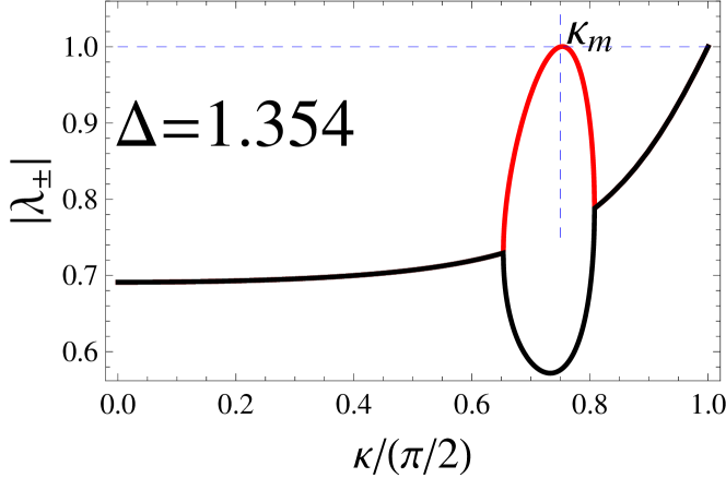
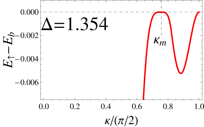
Figure 6: The same quantities as in Fig.5 but with $\Delta=\Delta_{c}=4-\sqrt{7}\sim 1.354$. Note the scale of the ordinate in the lower panel, showing the minute energy difference as compared with the overall energy scale of the system.

Edge modes with reentrance

We finally consider the case (iii): two solutions $\kappa_{m1}<\kappa_{m2}$ with $\Delta_{B}<\Delta_{4c}$. From eqs.(73) and (77) we obtain the relation

$$0<\kappa_{c1}<\kappa_{m1}<\kappa_{m2}<\kappa_{c2}<\pi/2$$ (81)

Hence we obtain the bulk momentum $\xi=0$ for both merging points. Then we expand $E_{\uparrow}-E_{\rm b}$ around merging points $\kappa_{mi}\ (i=1,2)$ as follows:

$$E_{\uparrow}(\kappa)-E_{\rm b}(\kappa,0)=a_{i}(\kappa-\kappa_{mi})^{2}+O\left((\kappa-\kappa_{mi})^{3}\right),$$ (82)

where the expansion coefficient is calculated as

$$a_{i} =\frac{4(A^{4}-8A^{2}+\Delta_{B}^{2})}{A^{2}\Delta_{B}}$$

$$\times\left[\frac{A^{2}-4}{A^{2}-8}+(-1)^{i}\frac{4\sqrt{A^{4}-8A^{2}+\Delta_{B}^{2}}}{\Delta_{4}(A^{2}-8)}\right]^{1/2}$$ (83)

Hence we have proven that the threshold of bulk excitation shares the same energy and velocity with edge mode, since the lowest order term of expansion is of second order.

At critical value of $\Delta_{B}=\Delta_{4c}$, we obtain $\kappa_{m}=\kappa_{m1}=\kappa_{m2}$, and both second and third order terms in eq.(82) tend to zero. Then the expansion around $\kappa_{m}$ begins from fourth order. This explains the nearly flat shape of $E_{\uparrow}-E_{\rm b}$ in Fig.6.

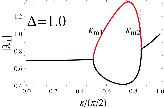
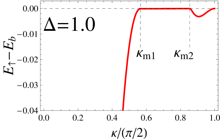
Figure 7: The same quantities as in Fig.5 but with $\Delta=1$. There is no edge mode for $\kappa$ between $\kappa_{m1}$ and $\kappa_{m2}$ where one of $|\lambda_{\pm}|$ exceeds unity.

Presence of two merging points causes novel phenomenon in zigzag edge mode. Figure 7 shows the parameter $|\lambda_{\pm}|$ and the energy difference as in previous cases. In the region $0<\kappa<\kappa_{m1}$ and $\kappa_{m2}<\kappa<\frac{\pi}{2}$, we obtain $|\lambda_{\pm}|<1$ and $E_{\uparrow}-E_{\rm b}<0$. Namely, the edge mode has two separate momentum ranges of its existence. The normal edge state (I) starts from zone center ($\kappa=0$), and vanishes at an intermediate point $\kappa=\kappa_{m1}$. In addition the reentrant part (II) appears near the zone boundary: $\kappa_{m2}<\kappa<\frac{\pi}{2}$. The reentrant edge mode has only marginally lower energy than lowest bulk excitation, which approximatively obeys $E_{\uparrow}-E_{\rm b}\propto(\kappa-\kappa_{m2})^{2}$. In the momentum range $\kappa_{m1}\leq\kappa\leq\kappa_{m2}$, the edge mode disappears since one of $|\lambda_{\pm}|$ exceeds unity.

Let us summarize the results for different $\Delta$ with fixed $A$ shown in Figs. 5, 6 and 7. As $\Delta$ increases from zero, the two separate regions for the edge modes widen in momentum space simultaneously. Namely, both $\kappa_{m1}$ and $\pi/2-\kappa_{m2}$ increase, while $\kappa_{m2}-\kappa_{m1}$ decreases with increasing $\Delta$. At critical $\Delta_{c}$, the two regions merge ($\kappa_{m1}=\kappa_{m2}$), and the unbroken edge mode emerges that disappears only at the zone boundary.

4.4 Edge modes in TI-2 regime

Let us now consider the TI-2 regime with $\Delta_{B}>0$. Since the Hamiltonian $H(\mib k)$ has only a linear term of $\Delta_{B}$, the solution in the TI-2 regime can be obtained from that in the TI-1 regime by changing the sign of $\Delta_{B}$. This conversion was indeed made in §3 for the straight edge.

In the zigzag edge, the spectrum given by eq.(65) has a negative slope because of $\Delta_{B}>0$. Corresponding to eq.(41), the merging momentum $\kappa_{m}>0$ is obtained from the condition

$$\lambda_{-}=-1,$$ (84)

instead of eq.(71). Then we obtain

$$\cos{\kappa_{m}}=\frac{\Delta_{B}\pm\sqrt{\Delta_{B}^{2}-A^{2}\left(8-A^{2}\right)}}{8-A^{2}},$$ (85)

instead of eq.(73), and

$$\Delta_{4c}=A\sqrt{8-A^{2}}>0,$$ (86)

instead of eq.(74). It is clear that the resultant solution of $\kappa_{m}$ is the same as that in TI-1 range with the same $|\Delta_{B}|$. Similarly, one can check that all relevant quantities such as $\kappa_{m1},\kappa_{m2},\kappa_{c1},\kappa_{c2}$ also have the same correspondence. The expression given by eqs.(79) and (82) remains valid, which means that the difference is now positive. This is naturally understood since the edge mode $E_{\uparrow}(\kappa)$ has the negative slope.

5 Summary and discussion

We have analytically obtained spectrum and wave function of helical edge states for the BHZ model by identifying the annihilator for each case of (1,0) and (1,1) edges. The simplicity of the BHZ model has allowed us to obtain the complete information of the edge modes. Let us finally consider the case $A>2$. In the straight edge, $\lambda_{\pm}$ are always real in this case. Except for this difference, the property of the edge mode spectrum remains the same. In the zigzag edge, the case $A>\sqrt{8}$ allows no solution for merging momentum $\kappa_{m}$. This means the edge mode is present up to the zone boundary.

Edge spectrum shows different properties depending on edge geometry. In (1,0)-edge case, edge spectrum is proportional to $\sin k$. As the sign of $\Delta_{B}$ changes from negative to positive, the main location of edge mode moves from the center of the 1D BZ to the boundary. This movement is associated with the change of location of the bulk energy gap.

For the (1,1) edge, we have obtained the spectrum in the form of $\pm\Delta_{B}\sin{\theta(\kappa)}$, where $\theta(\kappa)$ is an odd function of momentum $\kappa$. Since $\theta(\kappa)$ does not depend on $\Delta_{B}$ as shown in eqs.(61) and (62), $\Delta_{B}$ appears only as the scale factor in the spectrum. With $\Delta_{B}=0$, the edge modes become completely flat for the whole Brillouin zone, and two-fold degenerate as a consequence of the time-reversal symmetry.

The edge mode in the (1,1) geometry contains a novel reentrant part with extremely small binding energy. As seen from Fig.7, the binding energy for the reentrant part is only $10^{-3}$ of the overall energy. Except for many-body phenomena such as superconductivity and Kondo effect, we have been unaware of emergence of such extraordinary different energy scale. In spite of the tiny binding energy, the decay of the wave function toward inside the system looks quite normal, as judged by $|\lambda_{\pm}|$ which deviates clearly from unity.

Mathematically speaking, the tiny binding energy stems from the following factors:
(i) The zone boundary $\kappa=\pi/2$ is a special point where the edge mode merges with bulk excitations.
(ii) Group velocity of the edge mode is the same as that of threshold excitation in the bulk at the merging point.
Let us assume $\kappa\geq 0$ for simplicity. The condition (ii) requires the energy difference $E_{\uparrow}-E_{\rm b}$ to be proportional to $(\kappa-\pi/2)^{2}$ near the zone boundary, and simultaneously to $(\kappa-\kappa_{m2})^{2}$ near the critical momentum. Hence in the intervening region $\kappa_{m2}<\kappa<\pi/2$, the growth of $E_{\uparrow}-E_{\rm b}$ is constrained from both ends. Provided $\pi/2-\kappa_{m2}\sim 0.1\pi$, we obtain the scaling factor $\sim 10^{-2}$ from the quadratic dependence of $E_{\uparrow}-E_{\rm b}$. It is hoped that more physical explanation can be provided in the near future why the binding energy is so small.

References

- [1] C.L.Kane and E.J. Mele: Phys. Rev. Lett. 95, 146802 (2005).
- [2] C.L. Kane and E.J. Mele: Phys. Rev. Lett. 95, 226801 (2005).
- [3] L. Fu, C.L. Kane and E.J. Mele: Phys. Rev. Lett. 98, 106803 (2007).
- [4] L. Fu and C.L. Kane: Phys. Rev. B 76, 045302 (2007).
- [5] B.A. Bernevig and S.C. Zhang: Phys. Rev. Lett. 96, 106802 (2006).
- [6] B. A. Bernevig, T. L. Hughes and S.-C. Zhang: Science 314, 1757 (2006).
- [7] H. Zhang, C.-X. Liu, X.-L. Qi, X. Dai, Z. Fang and S.C. Zhang: Nat. Phys. 5, 438 (2009).
- [8] M. König, S. Wiedmann, C. Brüne, A. Roth, H. Buhmann, L.W. Molenkamp, X.-L. Qi, and S.C. Zhang: Science 318, 766 (2007).
- [9] D. Hsieh, D. Qian, L. Wray, Y. Xia, Y.S. Hor, R.J. Cava and M.Z. Hasan: Nature 452, 970 (2008).
- [10] Y. Xia, D. Qian, D. Hsieh, L. Wray, A. Pal, H. Lin, A. Bansil, D. Grauer, Y.S. Hor, R.J. Cava and M.Z. Hasan: Nat. Phys. 5, 398 (2009).
- [11] M. König, H. Buhmann, L.W. Molenkamp, T.L. Hughes, C.X Liu, X.-L Qi and S.C Zhang: J. Phys. Soc. Jpn 77, 031007 (2008).
- [12] C. Wu, B.A. Bernevig, and S.C. Zhang: Phys. Rev. Lett. 96, 106401 (2006).
- [13] C. Xu and J. Moore, Phys. Rev. B 73, 045322 (2006).
- [14] B. Zhou, H.-Z. Lu, R.-L. Chu, S.-Q. Shen, and Q. Niu: Phys. Rev. Lett. 101, 246807 (2008).
- [15] E.B. Sonin: arXiv:1006.5218.
- [16] M. Fujita, K. Wakabayashi, K. Nakada, and K. Kusakabe: J. Phys. Soc.Jpn. 65,1920 (1996).
- [17] K. Nakada and M. Fujita: Phys. Rev. B 54, 17954 (1996).
- [18] K. Imura, A. Yamakage, S. Mao, A. Hotta and Yoshio Kuramoto: arXiv:1004.5019; Phys. Rev. B in press.
- [19] M. Creutz and I. Horvath:Phys. Rev. D 50, 2297 (1994).
- [20] M. Creutz: Rev. Mod. Phys. 73, 119 (2001).
- [21] H.B. Nielsen and M. Ninomiya: Nucl. Phys. B 185 20 (1981); ibid. 193 173 (1981).