Abstract

With the early afterglow localizations of gamma-ray burst positions made by Swift, the clear delimitation of the prompt phase and the afterglow is not so obvious any more. It is important to see weather the two phases have the same origin or they stem from different parts of the progenitor system. We will combine the two kinds of gamma-ray burst data from the Swift-XRT instrument (windowed timing and photon counting modes) and from BAT. A thorough desription of the applied procedure is given. We apply various binning techniques to the different data: Bayes blocks, exponential binning and signal-to-noise type of binning. We present a handful of flux curves and some possible applications.

1 Introduction

Gamma-ray bursts are the most energetic phenomenon in the Universe. After their discovery (Klebesadel et al., 1973), and the detection of the first counterpart in other wavelengths than gamma now the Swift satellite (Gehrels et al. 2004) is almost routinely observing X-ray afterglows. In the study of GRB prompt emission and afterglow, it is a straightforward idea to combine flux curves of GRBs from gamma-ray and X-ray data. A wide spectral coverage leads to a more complete picture of the phenomenon. In our analysis have extrapolated the gamma-ray flux into the X-ray band to have a commond ground for analysis. It can be done the other way around, extrapolating the X-ray flux to the BAT energy range. Most bursts in our sample come from the long and possibly the intermediate duration group (Horváth 1998, Balázs et al. 1998, Balázs et al. 1999, Horváth 2002, Horváth et al. 2008, Řípa et al. 2009)

2 Data reduction and binning

Swift gathers $\gamma$-ray and X-ray data relevant for our analysis. We choose three different approaches to bin the flux curves: Bayesian method for the gamma-ray data, equal binning in logarithmic coordinates in the case of the windowed timing (WT) XRT data and a signal-to-noise type of binning in the case of photon counting (PC) XRT data. The flux curves and the spectra were generated using standard HEASoft tools and the most recent calibration database. Initial calibration was made using xrtpipeline and batgrbproduct pipeline scripts with the latest calibration databases.

In gamma-rays the results of the primary pipeline processing contain, among others, a $64$ ms resolution gamma-ray flux curve. This was used as the input to the Bayesian block analysis. We cut our combined $15-150$ keV flux curve using Bayes blocks as presented in Scargle (1998). We set a large prior for the algorithm so it will stop at an early point (which corresponds to a small number of change points) making sure that we have enough resolution for each of the bins. After deducing the time intervals we have used batbinevt to bin the data and get a raw spectrum (pha) file. The further steps recommended in the BAT analysis thread were also carried out. For each interval, we created the appropriate response matrices and fitted both a power law and a power law with a high-energy cutoff. We use the criterion from Sakamoto et al. (2008) to choose between the two models. If the $\chi^{2}$ improves by more than $6$ by using a cutoff power law, we use the latter instead of the simple power law model. The next step is to extrapolate the model from the gamma-ray band ($15-150$ keV) into the X-ray band ($0.3$ - $10$ keV).

In X-rays the WT mode is active when the count rate of the source is high (over $\sim 10$ counts/s). This means we have a good signal-to-noise ratio and we can bin the counts in equal bins in logarithmic space. We have fitted a spectrum for the whole duration of the WT mode and got a conversion factor from rates to flux. There is a more detailed description of the procedure in the next section.

For the PC mode we bin our data to have a signal-to-noise ratio of at least $3$. We do this by incrementing the endpoint of our interval in time until the count rate reaches the required level. At this point we store this interval and repeat the procedure until the end of the observing period. We correct for the pile-up in the detector as described in Vaughan et al. (2006) for the PC mode. For the WT mode pileup correction is made according to Romano et al. (2008)

The next step is to convert the count rates to flux. To do this, we divide the cumulative flux curve in $n$ parts, each with equal number of counts. $n$ is chosen by hand depending on the intensity of the afterglow from $2$ to $6$. For each time slice we fit a spectrum to get the count equivalent in erg/cm². The spectra are fitted with Xspec using individual anciliary response functions and the most recent response function available. We used an absorbed power law model of the form:

$$(\mathrm{wabs}_{G})\times(\mathrm{zwabs}_{S})\times\mathrm{(powerlaw)}.$$

The absorbing column density (NH) of the Milky Way was taken from Dickey et Lockman (1990) (denoted here by $\mathrm{wabs}_{G}$), and, where redshift was known, the source absorbtion was also fitted (denoted here by $\mathrm{zwabs}_{S}$). If the redshift was unknown $\mathrm{zwabs}_{S}$ was substituted with a simple absorbing $\mathrm{wabs}_{S}$ component. The spectra were binned using grppha so all channels had minimum $20$ counts.

Evans et al. (2007) use the same method, but they get the conversion factor (erg/cm²/s equivalent of $1$ count/s ) by integrating over the entire spectrum (corresponding to $n=1$). We report here that our conversion factors are in good agreement with those in Evans et al. (2007) and their related web-page.

3 Interesting cases

Here we present several GRBs to illustrate our method of binning and combining data. For now, we include only bursts from the long and intermediate duration population. The behaviour of the afterglow requires the use of a log scale but several GRBs have significant flux before the trigger (precursors with $t<T_{trigger}=0$). For this reason we choose to include a shift in the time axis where necessary.

Another way of examining the problem is to consider gamma-ray and X-ray photon indices. If the emission stems from the same population of electrons, we would expect the two types of indices to be equal within errors. The measurements should be carried out roughly at same time. We have taken a sample 10 bright Swift bursts and compared the two indices. We found that there was a visible discrepancy. (Figure 1)

Figure 1: Photon indices from the late prompt emission phase and the early afterglow phase. The continuous line represents equality between the two parameters

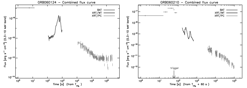
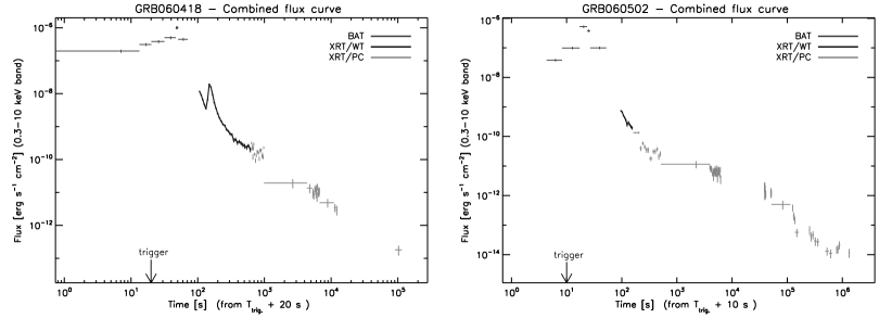
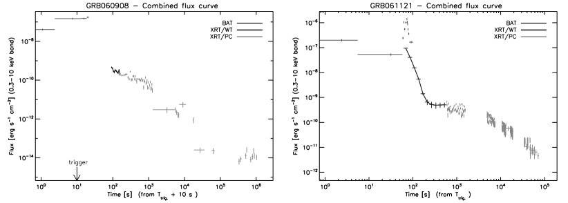
Figure 2: A few examples of combined flux curves of Swift GRBs.

4 Discussion and Conclusion

We have selected a few bright GRBs (Figure 2) to present our binning method for data from two bands. There are cases where the possible extrapolation of the WT mode data seems to match the gamma-ray flux curve (for the first three GRBs: 060210, 060418 and 060502). This could be proof of a connection between the processes which govern the prompt phase and the processes of the early afterglow. It looks possible that the steep decline is indeed a sequel of the prompt phase seen in X-rays. No such claim can be made for the following two events (060604 and 060908) because of the scarceness of the data. At the last two events (061121 and 060124) however, there is an apparent discrepancy between the gamma-ray curve and the X-ray curve. This discrepancy is best seen at GRB061121. This could mean the extrapolation of the gamma-ray spectrum was not adequate.

ACKNOWLEDGMENTS. This research is supported from Hungarian OTKA grant K077795.

REFERENCES

Balázs, L.G., Mészáros, A. and Horváth, I. 1998, A&A, 339, 1 Balázs, L.G., Mészáros, A., Horváth, I. and Vavrek, R., 1999, A&AS, 138, 417 Dickey, J.M. and Lockman, F.J., 1990, ARA&A, 28, 215 Evans, P.A., Beardmore, A.P., Page, K.L. et al., 2007, A&A, 469, 379 Gehrels, N., Chincarini, G., Giommi, P. et al., 2004, ApJ 611, 1005 Horváth, I., 1998, ApJ, 508, 757 Horváth, I., 2002, A&A, 392, 791 Horváth, I., 2009, Ap&SS, 323, 83 Klebesadel, R.W., Strong, I.B. and Olson, R.A., ApJ, 182, 85 Řípa, J., Mészáros, A., Huja, D. 2009, A&A, 498, 399 Romano, P., Campana, S., Chincarini, G. et al., 2006, A&A, 456, 917 Sakamoto, T., Barthelmy, S.D., Barbier, L. et al., 2008, ApJ, 175, 179 Scargle, J. D., 1998, ApJ, 504, 405 Vaughan, S., Goad, M.R., Beardmore, A.P. et al., 2006, ApJ, 638, 920