Resummation of large logarithms in the heavy quark effects
on the parton distributions inside the virtual photon

Abstract

We discuss the resummation of the large logarithmic terms appearing in the heavy quark effects on parton distribution functions inside the virtual photon. We incorporate heavy quark mass effects by changing the initial condition of the leading-order DGLAP evolution equation. In a certain kinematical limit, we recover the logarithmic terms of the next-to-leading order heavy quark effects obtained in the previous work. This method enables us to resum the large logarithmic terms due to heavy quark mass effects on the parton distributions in the virtual photon. We numerically calculate parton distributions using the formulae derived in this work, and discuss the property of the resummed heavy quark effects.

I Introduction

The Large Hadron Collider (LHC) LHC has restarted at the CERN for the purpose of discovering the Higgs boson, the new physics beyond the standard model, and investigating the detailed information for the quark gluon plasma, the B meson decays and so on. The precise measurement will be needed to confirm the discovery of the Higgs boson and searching the beyond standard model at the electron-positron collider like International Linear Collider (ILC) ILC and Super KEK-B KEKB . In such a case, we have to know the behaviour of quantum chromodynamics (QCD) at high energies because of the largeness of QCD corrections.

There is a well-known fact that the cross section of the two-photon processes $e^{+}e^{-}\to\gamma^{*}\gamma^{*}\to e^{+}e^{-}+\mbox{hadrons}$ dominates over that of the one-photon annihilation processes $e^{+}e^{-}\to\gamma^{*}\to\mbox{hadrons}$ in the electron-positron collisions at high energies twophoton . Let us consider the two-photon processes where both of the outgoing $e^{+}$ and $e^{-}$ are detected and one of the virtual photons is far off-shell with mass squared $q^{2}=-Q^{2}$, while the other photon is close to the on-shell with mass squared $p^{2}=-P^{2}$. In this kinematical region, the former photon is called the ‘probe photon’ and the latter one is called the ‘target photon’ (see Fig. 1).

We can regard this two-photon process as the deep-inelastic scattering in the electron-positron collision where the target is a photon rather than a nucleon. In this point of view, we can define the photon structure functions as the analogues of the nucleon structure functions, and the photon structure functions are predicted by the quantum electrodynamics (QED) and QCD. One of the difference between the nucleon structure functions and the photon structure functions is the target mass ($P^{2}$) dependence. The $P^{2}$ is not fixed for the virtual photon case, on the other hand, $P^{2}$ is fixed for the nucleon case. There are many good reviews for the theoretical as well as the experimental works for photon structure functions, for example, see Review .

Figure 1: Deep inelastic scattering for virtual photons in $e^{+}e^{-}$ collision.

The real ($P^{2}=0$) unpolarised photon structure functions $F^{\gamma}_{2}(x,Q^{2})$ and $F^{\gamma}_{L}(x,Q^{2})$ were investigated in the parton model (PM) QPM , in the perturbative QCD (pQCD) based on the operator product expansion (OPE) CHM supplemented by the renormalisation group (RG) method Witten ; BB , and also on the QCD improved PM Altarelli powered by the parton evolution equation Dewitt ; GR1983 ; MVV2002 ; MVV2004NNLOpart3 . The real polarised photon structure function $g^{\gamma}_{1}(x,Q^{2})$ was investigated with pQCD in polg1LO for the leading-order (LO), and for the next-to-leading order (NLO) in polg1NLO1 ; GRS2001 .

The virtual ($P^{2}\neq 0$) unpolarised photon structure functions $F^{\gamma}_{2}(x,Q^{2},P^{2})$ and $F^{\gamma}_{L}(x,Q^{2},P^{2})$ were also investigated by UW1 ; UW2 ; Rossi ; BA ; Chyla in the kinematical region

$$\Lambda^{2}\ll P^{2}\ll Q^{2},$$ (1)

where $\Lambda$ is the fundamental QCD scale parameter. The advantage to study the virtual photon target for the kinematical region (1) is that we can calculate the whole shape and magnitude of the photon structure functions entirely by the perturbative method. Based on the recent results for the three-loop calculation for the photon-quark and the photon-gluon splitting functions (anomalous dimensions) MVV2004NNLOpart3 ; MVV2004NNLOpart1 ; MVV2004NNLOpart2 , the unpolarised virtual photon structure function $F^{\gamma}_{2}(x,Q^{2},P^{2})$ ($F^{\gamma}_{L}(x,Q^{2},P^{2})$) was studied to the NNLO (to the NLO) USU2007 ; KSUU2008 , and the polarised virtual photon structure function $g^{\gamma}_{1}(x,Q^{2},P^{2})$ was studied to the NLO in GRS2001 ; SU1999 ; BSU2002 ; SUU2006 .

In the parton picture, the photon structure function is expressed as the convolution of the parton distribution function (PDF) in the virtual photon with the coefficient functions in the OPE formalism. We can also give the definite prediction for the PDFs inside the photon, which we call “photon PDFs” for short, in the present paper. The theoretical calculations were done for unpolarised and polarised photon PDFs in Rossi ; DG ; GRStratmann ; Fontannaz ; SU2000 ; USU2009 . However, these calculations in MVV2004NNLOpart3 ; USU2007 ; SU2000 ; USU2009 were assumed that all quarks in the virtual photon are massless. When the centre of mass energy is enough large to produce heavy quarks (with mass $m$), i.e. $(p+q)^{2}\geq 4m^{2}$, the heavy quark mass effects should be taken into account. In the case of the nucleon target, the heavy quark mass effects were studied by a method based on the OPE in Buza-etal1999 .

Many authors have investigated the heavy quark mass effects in the photon structure functions GR1983 ; GRS2001 ; GRStratmann ; Fontannaz ; AFG ; GRSch1999 ; SSU2002 ; CJKL2003 ; CJK2004 ; GRV1992b ; KSUU2009 . The heavy quark mass effects were included in the theoretical calculation for the PDFs of the real photon in Ref. Fontannaz ; AFG by changing the initial condition of the DGLAP equation, for the virtual photon PDFs in Ref. KSUU2009 ; KSUU2010 by using the OPE formalism supplemented by the mass-independent DGLAP equation. In Refs. Fontannaz ; AFG , the heavy quark mass effects are incorporated by changing the initial condition. On the other hand, in Refs. KSUU2009 ; KSUU2010 , the heavy quark mass effects are included by evaluating the finite matrix elements of the heavy-quark operators between the photon states. Recently we have found that the DGLAP equation with modified initial condition for the heavy quark PDF Fontannaz ; AFG leads to the similar results which we have obtained by the OPE method KSUU2009 ; KSUU2010 as we have mentioned before.

In the present paper, we adopt the alternative way to treat the heavy quark mass effects on the virtual photon PDFs by setting the initial condition for the heavy quark PDF in the DGLAP evolution equation, which amounts to sum up the large logarithmic terms. Through this prescription we try to improve the previous results for the heavy quark mass effects.

In the next section, we discuss the basic formalism of the evolution equation for virtual photon PDFs. We derive the explicit expressions for the virtual photon PDFs with the heavy quark mass effects in which the large logarithmic terms are resummed in section III. In section IV, we present the numerical calculation of the results for photon PDFs. The final section is devoted to the conclusions.

II Basic Formalism

First let us discuss the basic formalism of the evolution equation for the PDFs in the virtual photon to the leading-order (LO) in QCD. We consider the system with $n_{f}$ quarks and decompose it into two groups, $n_{f}-1$ light (i.e. massless) quarks and a heavy quark. Let

$$q^{i}_{L}(x,Q^{2},P^{2}),\qquad q^{\gamma}_{H}(x,Q^{2},P^{2}),\qquad G^{\gamma}(x,Q^{2},P^{2}),\qquad\Gamma^{\gamma}(x,Q^{2},P^{2}),$$ (2)

be light quark distributions (with $i$ flavour and $i=1,\ldots,n_{f}-1$), heavy quark distribution, gluon distribution and photon distribution inside the virtual photon, respectively. All the PDFs $q_{i}^{\gamma}(x,Q^{2},P^{2})$ evolve from the virtuality of the target photon $P^{2}$ to the virtuality of the probe photon $Q^{2}$. At the LO of the QED coupling constant ($\mathcal{O}$($\alpha$); $\alpha=e^{2}/4\pi$), $\Gamma^{\gamma}(x,Q^{2},P^{2})$ does not evolve with respect to $Q^{2}$ and therefore we set $\Gamma^{\gamma}(x,Q^{2},P^{2})=\delta(1-x)$. Since light quarks are distinguished from other quarks only through their electromagnetic charge, it is good to change the flavour basis to the light singlet and the light nonsinglet. We define the light singlet $q^{\gamma}_{Ls}$ and the light nonsinglet $q^{\gamma}_{Lns}$ by the equations

$$q^{\gamma}_{Ls}\equiv\sum_{i=1}^{n_{f}-1}q^{i}_{L}~{},\qquad q^{\gamma}_{Lns}\equiv\sum_{i=1}^{n_{f}-1}e^{2}_{i}\Bigl{(}q^{i}_{L}-\frac{1}{n_{f}-1}q^{\gamma}_{Ls}\Bigr{)},$$ (3)

where $e_{i}$ is the electromagnetic charge for $i$-th flavour quark in the unit of proton charge. The photon PDFs are described by a row vector $\mbox{\boldmath$q$}^{\gamma}$ which satisfies the inhomogeneous DGLAP evolution equation

$$\frac{d}{d\ln Q^{2}}\mbox{\boldmath$q$}^{\gamma}(x,Q^{2},P^{2}) = \int_{x}^{1}\frac{dy}{y}\mbox{\boldmath$q$}(y,Q^{2},P^{2})\hat{\mbox{\boldmath$P$}}\left(\frac{x}{y},Q^{2}\right)+\mbox{\boldmath$k$}(x,Q^{2}),$$ (4)

where the row vector $\mbox{\boldmath$q$}^{\gamma}(x,Q^{2},P^{2})$ is defined as

$$\mbox{\boldmath$q$}^{\gamma}=\left(q^{\gamma}_{Ls},q^{\gamma}_{H},G^{\gamma},q^{\gamma}_{Lns}\right),$$ (5)

and another row vector $\mbox{\boldmath$k$}^{\gamma}(x,Q^{2})=(k_{Ls},k_{H},k_{G},k_{Lns})$ denotes the photon-parton splitting functions. The $4\times 4$ matrix $\hat{\mbox{\boldmath$P$}}(z,Q^{2})$ is expressed as

$$\hat{\mbox{\boldmath$P$}}(z,Q^{2})=\begin{pmatrix}P_{LL}^{S}(z,Q^{2})&P_{HL}(z,Q^{2})&P_{GL}(z,Q^{2})&0\\ P_{LH}(z,Q^{2})&P_{HH}(z,Q^{2})&P_{GH}(z,Q^{2})&0\\ P_{LG}(z,Q^{2})&P_{HG}(z,Q^{2})&P_{GG}(z,Q^{2})&0\\ 0&0&0&P_{LL}^{NS}(z,Q^{2})\end{pmatrix},$$ (6)

where each element $P_{AB}$ means a splitting function of $B$ parton to $A$ parton.

One can solve the DGLAP equation (4) by introducing the moments of the photon PDFs QPM . Here we discuss the procedure briefly. By taking the moment, one obtains the equation

$$\frac{d}{d\ln Q^{2}}\mbox{\boldmath$q$}^{\gamma}(n,Q^{2},P^{2}) = \mbox{\boldmath$k$}(n,Q^{2})+\mbox{\boldmath$q$}^{\gamma}(n,Q^{2},P^{2})\hat{\mbox{\boldmath$P$}}\left(n,Q^{2}\right),$$ (7)

where an $n$-th moment $f(n)$ of a function $f(x)$ is defined by

$$f(n)\equiv\int_{0}^{1}dxx^{n-1}f(x).$$ (8)

Then we introduce the variable $t$ as FP1

$$t = \frac{2}{\beta_{0}}\ln\frac{\alpha_{s}(P^{2})}{\alpha_{s}(Q^{2})},$$ (9)

instead of $Q^{2}$. We expand $\mbox{\boldmath$k$}_{n}=\mbox{\boldmath$k$}(n,Q^{2})$, $\hat{\mbox{\boldmath$P$}}_{n}=\hat{\mbox{\boldmath$P$}}(n,Q^{2})$ and $\mbox{\boldmath$q$}^{\gamma}_{n}=\mbox{\boldmath$q$}^{\gamma}(n,Q^{2},P^{2})$ in powers of the QED coupling constant $\alpha$ as well as the QCD coupling constant $\alpha_{s}$ as follows

$$\mbox{\boldmath$k$}_{n} = \frac{\alpha}{2\pi}\mbox{\boldmath$k$}^{(0)}_{n}+\frac{\alpha}{2\pi}\frac{\alpha_{s}(t)}{2\pi}\mbox{\boldmath$k$}^{(1)}_{n}+\cdots,$$ (10)

$$\hat{\mbox{\boldmath$P$}}_{n} = \frac{\alpha_{s}(t)}{2\pi}\hat{\mbox{\boldmath$P$}}^{(0)}_{n}+\left(\frac{\alpha_{s}(t)}{2\pi}\right)^{2}\hat{\mbox{\boldmath$P$}}^{(1)}_{n}+\cdots,$$ (11)

$$\mbox{\boldmath$q$}^{\gamma}_{n} = \mbox{\boldmath$q$}^{\gamma(0)}_{n}+\mbox{\boldmath$q$}^{\gamma(1)}_{n}+\cdots,$$ (12)

where the $\alpha_{s}$ dependence appears in $\mbox{\boldmath$q$}^{\gamma}_{n}$ implicitly with the notation USU2007 , and $\mbox{\boldmath$q$}^{\gamma(0)}_{n}$ and $\mbox{\boldmath$q$}^{\gamma(1)}_{n}$ correspond to the LO and NLO solutions, respectively. One finally obtains the LO solution $\mbox{\boldmath$q$}^{\gamma(0)}_{n}$ for the DGLAP equation (7) as

$$\mbox{\boldmath$q$}^{\gamma(0)}_{n}(t) = \frac{\alpha}{8\pi\beta_{0}}\frac{4\pi}{\alpha_{s}(t)}\mbox{\boldmath$K$}_{n}^{(0)}\sum_{i}P_{i}^{n}\frac{1}{1+d_{i}^{n}}\left\{1-r^{1+d_{i}^{n}}\right\}+\mbox{\boldmath$q$}^{\gamma(0)}_{n}(0)\sum_{i}r^{d_{i}^{n}}P_{i}^{n},$$ (13)

where $r$ is the ratio of QCD couplings which is defined by

$$r=\frac{\alpha_{s}(t)}{\alpha_{s}(0)}=\frac{\alpha_{s}(Q^{2})}{\alpha_{s}(P^{2})}.$$ (14)

Now the last term of (13) is determined by the initial condition. Although we usually set $\mbox{\boldmath$q$}^{\gamma(0)}_{n}(0)=0$, as we took in our previous paper KSUU2010 , we change the initial condition for the heavy quark PDF and we will discuss the relation between this modification and resummation in the next section.

$\beta_{0}$ and $\beta_{1}$ appears in the perturbative expansion of the QCD running coupling constant of the QCD running coupling constant

$$\frac{d}{d\ln Q^{2}}\alpha_{s}(Q^{2}) = -\beta_{0}\frac{\alpha_{s}^{2}(Q^{2})}{4\pi}-\beta_{1}\frac{\alpha_{s}^{3}(Q^{2})}{(4\pi)^{2}}+\cdots,$$ (15)

with $\beta_{0}=11-2n_{f}/3$ and $\beta_{1}=102-38n_{f}/3$. The relation between $\mbox{\boldmath$k$}_{n}^{(0)}$ and $\mbox{\boldmath$K$}_{n}^{(0)}$ is given by,

$$\mbox{\boldmath$k$}_{n}^{(0)} = \frac{1}{4}\mbox{\boldmath$K$}_{n}^{(0)},$$ (16)

where the elements of row vector $\mbox{\boldmath$K$}_{n}^{(0)}=\left(K_{Ls}^{0,n},K_{H}^{0,n},K_{G}^{0,n},K_{Lns}^{0,n}\right)$ are evaluated to be

$$K_{Ls}^{0,n} = 24(n_{f}-1)\langle e^{2}\rangle_{L}k_{n}^{0},$$ (17)

$$K_{H}^{0,n} = 24e_{H}^{2}k_{n}^{0},$$ (18)

$$K_{G}^{0,n} = 0,$$ (19)

$$K_{Lns}^{0,n} = 24(n_{f}-1)(\langle e^{4}\rangle_{L}-\langle e^{2}\rangle_{L}^{2})k_{n}^{0},$$ (20)

$$k_{n}^{0} = \frac{n^{2}+n+2}{n(n+1)(n+2)},$$ (21)

where the charge factors for quadratic term $\langle e^{2}\rangle_{L}$ and for quartic term $\langle e^{4}\rangle_{L}$ are defined by

$$\langle e^{2}\rangle_{L} \equiv \frac{1}{n_{f}-1}\sum_{i=1}^{n_{f}-1}e_{i}^{2},\hskip 56.9055pt\langle e^{4}\rangle_{L}\equiv\frac{1}{n_{f}-1}\sum_{i=1}^{n_{f}-1}e_{i}^{4}.$$ (22)

Note that $K_{Ls}^{0,n}+K_{H}^{0,n}=K_{\psi}^{0,n}$, and $K_{\psi}^{0,n}$ is the usual flavour-singlet anomalous dimension for $n_{f}$ massless quarks. The relation between $\hat{\mbox{\boldmath$P$}}_{n}^{(0)}$ and $P_{i}^{n}$ is given by

$$\hat{\mbox{\boldmath$P$}}_{n}^{(0)} = -\frac{1}{4}\hat{\gamma}^{(0)}_{n}=-\frac{1}{4}\sum_{i=\psi,\pm,Lns}\lambda_{i}^{n}P_{i}^{n},$$ (23)

where $\hat{\gamma}^{(0)}_{n}$ is the one-loop hadronic anomalous dimension matrix, $\lambda_{i}^{n}=2\beta_{0}d_{i}^{n}$ ($i=\psi,\pm,Lns$) are the eigenvalues of $\hat{\gamma}^{(0)}_{n}$ which are given by

$$\lambda_{\psi}^{n} = \lambda_{Lns}^{n}=\gamma_{\psi\psi}^{0,n},$$ (24)

$$\lambda_{\pm}^{n} = \frac{1}{2}\left[\gamma_{\psi\psi}^{0,n}+\gamma_{GG}^{0,n}\pm\sqrt{(\gamma_{\psi\psi}^{0,n}-\gamma_{GG}^{0,n})^{2}+4\gamma_{\psi G}^{0,n}\gamma_{G\psi}^{0,n}}\right].$$ (25)

The $P_{i}^{n}$ are the projection matrices in the spectral decomposition for $\hat{\gamma}^{(0)}_{n}$ which satisfy the following relations:

$$P_{i}^{n}P_{j}^{n} = \delta_{ij}P_{i}^{n},~{}\hskip 28.45274pt\sum_{i}P_{i}^{n}=\bf{1}_{4\times 4},$$ (26)

where $i,j=\psi,\pm,Lns$ runs over the eigenvalues, and the explicit expressions are given by

$$P_{\psi}^{n} = \left(\begin{array}[]{ccc|c}\frac{1}{n_{f}}&-\frac{1}{n_{f}}&0&0\\ -\frac{n_{f}-1}{n_{f}}&\frac{n_{f}-1}{n_{f}}&0&0\\ 0&0&0&0\\ \hline\cr 0&0&0&0\end{array}\right)~{},\hskip 56.9055ptP_{Lns}^{n}=\left(\begin{array}[]{ccc|c}0&0&0&0\\ 0&0&0&0\\ 0&0&0&0\\ \hline\cr 0&0&0&1\end{array}\right),~{}$$ (35)

$$P_{\pm}^{n} = \frac{1}{\lambda_{\pm}^{n}-\lambda_{\mp}^{n}}\left(\begin{array}[]{ccc|c}\frac{n_{f}-1}{n_{f}}(\gamma_{\psi\psi}^{0,n}-\lambda_{\mp}^{n})&\frac{1}{n_{f}}(\gamma_{\psi\psi}^{0,n}-\lambda_{\mp}^{n})&\gamma_{G\psi}^{0,n}&0\\ \frac{n_{f}-1}{n_{f}}(\gamma_{\psi\psi}^{0,n}-\lambda_{\mp}^{n})&\frac{1}{n_{f}}(\gamma_{\psi\psi}^{0,n}-\lambda_{\mp}^{n})&\gamma_{G\psi}^{0,n}&0\\ \frac{n_{f}-1}{n_{f}}\gamma_{\psi G}^{0,n}&\frac{1}{n_{f}}\gamma_{\psi G}^{0,n}&\gamma_{GG}^{0,n}-\lambda_{\mp}^{n}&0\\ \hline\cr 0&0&0&0\end{array}\right)~{}.$$ (40)

The most important part in the present paper is $\mbox{\boldmath$q$}_{n}^{\gamma(0)}(0)$, which is the initial condition for the DGLAP Eq. (7). We usually set this term $\mbox{\boldmath$q$}^{\gamma(0)}_{n}(0)$ to be vanishing at the LO. However, we will find that the resummed expression of the logarithm term $\ln(m^{2}/P^{2})$ which appears as the heavy quark mass effects in Eq. (65) in Ref. KSUU2010 is recovered by changing the initial condition of the DGLAP Eq. (7) for the heavy quark component as discussed in the next section.

III Initial condition and resummation

In Ref. KSUU2010 it is shown that the additional terms for the moment of the PDF obtained by the OPE method are proportional to the LO renormalisation group parameters and the logarithmic terms. Therefore we can expect the possibility to derive the previous results by the LO evolution equation. We demonstrate it by changing the initial condition for the LO evolution equation.

III.1 A change in the initial condition for the heavy quark

The moment for the heavy quark component $q^{(0),n}_{H}(t)$ can be projected after some calculations by using the Eq. (13),

$$q_{H}^{(0),n}(t)/\frac{\alpha}{8\pi\beta_{0}} = \frac{4\pi}{\alpha_{s}(t)}\left[-\frac{1}{1+d_{\psi}^{n}}\left(\frac{1}{n_{f}}K_{\psi}^{n}-K_{H}^{0,n}\right)\left(1-r^{d_{\psi}^{n}+1}\right)+\frac{1}{n_{f}}K_{\psi}^{0,n}\sum_{\pm}\frac{1}{1+d_{\pm}^{n}}\frac{\gamma_{\psi\psi}^{0,n}-\lambda_{\mp}^{n}}{\lambda_{\pm}^{n}-\lambda_{\mp}^{n}}\left(1-r^{d_{\pm}^{n}+1}\right)\right]$$ (41)

$$\hskip 19.91684pt+\left[\frac{n_{f}-1}{n_{f}}r^{d_{\psi}^{n}}+\frac{1}{n_{f}}\sum_{\pm}\frac{\gamma_{\psi\psi}^{0,n}-\lambda_{\mp}^{n}}{\lambda_{\pm}^{n}-\lambda_{\mp}^{n}}r^{d_{\pm}^{n}}\right]\hat{q}_{H}^{(0),n}(0)/\frac{\alpha}{8\pi\beta_{0}},$$

where we denote $\sum_{\pm}f(\lambda_{\pm})\equiv f(\lambda_{+})+f(\lambda_{-})$ and $\hat{q}_{H}^{(0),n}$ in the last term should be determined later. As we mentioned previously, we change the initial condition of the DGLAP equation. Let us consider the following condition:

$$\mbox{\boldmath$q$}^{\gamma(0)}_{n}(t=0) = \left(0,\hat{q}_{H}^{(0),n},0,0\right),$$ (42)

where $\hat{q}_{H}^{(0),n}$ is the heavy-quark PDF evaluated at the scale $t=0~{}(Q^{2}=P^{2})$. This modification for the initial condition of the LO DGLAP equation corresponds to a kind of the heavy quark threshold effect, because the evolution for the heavy quark component is suppressed by this condition. The initial condition $\hat{q}_{H}^{(0),n}$ is determined by the equation

$$\hat{q}_{H}^{(0),n}(t_{m}) = 0,$$ (43)

$$t_{m} = \frac{2}{\beta_{0}}\ln\frac{\alpha_{s}(P^{2})}{\alpha_{s}(m^{2})}.$$ (44)

Setting $t=t_{m}$ in Eq. (41), we obtain the following result:

$$\hat{q}_{H}^{(0),n}(0)/\frac{\alpha}{8\pi\beta_{0}} = -H_{n}(t_{m})/J_{n}(t_{m}),$$ (45)

where the functions $H_{n}(t_{m})$ and $J_{n}(t_{m})$ are defined by

$$H_{n}(t_{m}) = \frac{4\pi}{\alpha_{s}(t_{m})}\left[-\frac{1}{1+d_{\psi}^{n}}\left(\frac{1}{n_{f}}K_{\psi}^{n}-K_{H}^{0,n}\right)\left(1-r^{d_{\psi}^{n}+1}_{m}\right)\right.$$ (46)

$$\left.\hskip 42.67912pt+\sum_{\pm}\frac{1}{1+d_{\pm}^{n}}\frac{1}{n_{f}}K_{\psi}^{0,n}\frac{\gamma_{\psi\psi}^{0,n}-\lambda_{\mp}^{n}}{\lambda_{\pm}^{n}-\lambda_{\mp}^{n}}\left(1-r^{d_{\pm}^{n}+1}_{m}\right)\right],$$

$$J_{n}(t_{m}) = \frac{n_{f}-1}{n_{f}}r_{m}^{d_{\psi}^{n}}+\frac{1}{n_{f}}\sum_{\pm}\frac{\gamma_{\psi\psi}^{0,n}-\lambda_{\mp}^{n}}{\lambda_{\pm}^{n}-\lambda_{\mp}^{n}}r_{m}^{d_{\pm}^{n}},$$ (47)

and here $r_{m}=\alpha_{s}(t_{m})/\alpha_{s}(0)$ corresponds to the ratio between the QCD running coupling at the scale of the heavy quark mass and that of the renormalisation scale for the photon matrix element in OPE formalism. See the Appendix A for the explicit expressions of the PDFs in the virtual photon including the resummed mass effects.

If we denote the variation terms as $\Delta q_{i}^{\gamma(0),n}(t)$ which are due to the heavy quark effects, then we recover the fixed order (NLO QCD + heavy quark mass effects) results as given by

$$\Delta q_{Ls}^{\gamma(0),n}(t)/\frac{\alpha}{8\pi\beta_{0}} = \Delta\hat{A}_{Ls}^{n,\psi}\left(1-r^{d_{\psi}^{n}}\right)+\sum_{\pm}\Delta\hat{A}_{Ls}^{n,\pm}\left(1-r^{d_{\pm}^{n}}\right),$$ (48)

$$\Delta\hat{A}_{Ls}^{n,\psi} = \frac{n_{f}-1}{n_{f}}2\beta_{0}\Delta\tilde{A}_{H}^{n},$$

$$\Delta\hat{A}_{Ls}^{n,\pm} = -\frac{n_{f}-1}{n_{f}}\frac{\gamma_{\psi\psi}^{0,n}-\lambda_{\mp}^{n}}{\lambda_{\pm}^{n}-\lambda_{\mp}^{n}}2\beta_{0}\Delta\tilde{A}_{H}^{n},$$

$$\Delta q_{H}^{\gamma(0),n}(t)/\frac{\alpha}{8\pi\beta_{0}} = \Delta\hat{A}_{H}^{n,\psi}\left(1-r^{d_{\psi}^{n}}\right)+\sum_{\pm}\Delta\hat{A}_{H}^{n,\pm}\left(1-r^{d_{\pm}^{n}}\right)+\Delta\hat{C}_{n},$$ (49)

$$\Delta\hat{A}_{H}^{n,\psi} = -\frac{n_{f}-1}{n_{f}}2\beta_{0}\Delta\tilde{A}_{H}^{n},$$

$$\Delta\hat{A}_{H}^{n,\pm} = -\frac{1}{n_{f}}\frac{\gamma_{\psi\psi}^{0,n}-\lambda_{\mp}^{n}}{\lambda_{\pm}^{n}-\lambda_{\mp}^{n}}2\beta_{0}\Delta\tilde{A}_{H}^{n},$$

$$\Delta\hat{C}_{n} = 2\beta_{0}\Delta\tilde{A}_{H}^{n},$$

$$\Delta G^{\gamma(0),n}(t)/\frac{\alpha}{8\pi\beta_{0}} = \sum_{\pm}\Delta\hat{A}_{G}^{n,\pm}\left(1-r^{d_{\pm}^{n}}\right),$$ (50)

$$\Delta\hat{A}_{G}^{n,\pm} = -\frac{\gamma_{G\psi}^{0,n}}{\lambda_{\pm}^{n}-\lambda_{\mp}^{n}}2\beta_{0}\Delta\tilde{A}_{H}^{n},$$

$$\Delta q_{Lns}^{\gamma(0),n}(t)/\frac{\alpha}{8\pi\beta_{0}} = 0,$$ (51)

where $\hat{q}_{H}^{(0),n}(0)/\frac{\alpha}{8\pi\beta_{0}}=2\beta_{0}\Delta\tilde{A}_{H}^{n}$. The variation of operator matrix element $\Delta\tilde{A}_{H}^{n}$ is evaluated from the LO coupling $\alpha_{s}(t_{m})$ together with the LO anomalous dimension $K_{H}^{0,n}$ in our method. Neglecting the finite term (large mass limit), the variation of the operator matrix element is evaluated as

$$\Delta\tilde{A}_{H}^{n} = -\frac{1}{2}K_{H}^{0,n}\ln\frac{m^{2}}{P^{2}}=-12e_{H}^{2}\frac{n^{2}+n+2}{n(n+1)(n+2)}\ln\frac{m^{2}}{P^{2}}.$$ (52)

All the results in the large mass limit is consistent with that of the variation terms in Ref. KSUU2010 except for the mass-independent finite terms. It is impossible to recover these terms only through the DGLAP equation and these difference could be considered as the scheme-dependence for photon PDFs.

III.2 A certain limit

Next we consider the expression by taking a limit ($\Lambda^{2}\ll P^{2}\ll m^{2}$) in order to compare our results with those in Ref. KSUU2010 .

In terms of the LO running coupling constant

$$\alpha_{s}(Q^{2})=\frac{4\pi}{\beta_{0}}\frac{1}{\ln(Q^{2}/\Lambda^{2})},$$ (53)

the ratio $r_{m}$ can be written as

$$r_{m} = \frac{\alpha_{s}(m^{2})}{\alpha_{s}(P^{2})}=\frac{\ln(P^{2}/\Lambda^{2})}{\ln(m^{2}/\Lambda^{2})}=1-\frac{\ln(m^{2}/P^{2})}{\ln(m^{2}/\Lambda^{2})}\equiv 1-\epsilon,$$ (54)

where $\epsilon=\ln(m^{2}/P^{2})/\ln(m^{2}/\Lambda^{2})$. Considering the case of large-mass limit: $\ln(m^{2}/P^{2})\ll\ln(m^{2}/\Lambda^{2}$), we can set the region of $\epsilon$ as $\epsilon\ll 1$. Then we can expand $H_{n}(t_{m}),J_{n}(t_{m})$ in the modified initial condition term $q_{H}^{(0),n}$ up to $\mathcal{O}(\epsilon)$ as

$$H_{n}(t_{m}) = \frac{4\pi}{\alpha_{s}(t_{m})}K_{H}^{0,n}\left[~{}\epsilon+O(\epsilon^{2})~{}\right],$$ (55)

$$J_{n}(t_{m}) = 1+O(\epsilon),$$ (56)

where we have used $(1+\epsilon)^{d}\approx 1+d\epsilon$. By using the fact $\frac{4\pi}{\alpha_{s}(t_{m})}=\beta_{0}\ln\frac{m^{2}}{\Lambda^{2}}$, we obtain the result as

$$\hat{q}_{H}^{(0),n}(0)/\frac{\alpha}{8\pi\beta_{0}}\approx-\beta_{0}K_{H}^{0,n}\ln\frac{m^{2}}{P^{2}}\left[~{}1+O(\epsilon)~{}\right],$$ (57)

where the order of the neglected term $O(\epsilon)$ corresponds to the terms like $\ln^{k}(m^{2}/P^{2}),(k=1,2,3,\dots)$. We recover the results about the large logarithmic term due to the heavy quark mass effect which appears in the result by OPE formalism except for mass-independent finite terms. Therefore the equations (65),(66),(67), and (68) which we derived by the modification of the initial condition for the heavy PDF in the LO DGLAP equation are more general forms and the large logarithm terms are resummed. The resummed terms form compact power terms $(r_{m})^{d_{i}^{n}}$ in $\hat{q}^{\gamma(0),n}_{H}(0)$.

IV Numerical Results

One can obtain the various photon PDFs from their moments by the inverse Mellin transformation. We show the results of numerical calculation for the heavy quark PDF $q^{\gamma}_{H}$, the gluon PDF $G^{\gamma}$, the light singlet quark PDF $q^{\gamma}_{Ls}$ and the effective photon structure function $F^{\gamma}_{\rm eff}$. The last one, $F^{\gamma}_{\rm eff}$, is scheme-independent and is proportional to the total cross section of the two photon process. We consider the two cases which were measured in the experiments  PLUTO ; L3 . The first case (i) resides in the PLUTO energy region where we regard the charm quark as the heavy quark, the second case (ii) is in the L3 energy region where we regard the bottom quark as the heavy quark,

case (i) $$\hskip 14.22636ptn_{f}=4,~{}Q^{2}=5~{}\mbox{GeV}^{2},~{}P^{2}=0.35~{}\mbox{GeV}^{2},~{}m_{c}=1.3~{}\mbox{GeV},$$ (58)

case (ii) $$\hskip 14.22636ptn_{f}=5,~{}Q^{2}=120~{}\mbox{GeV}^{2},~{}P^{2}=3.7~{}\mbox{GeV}^{2},~{}m_{b}=4.2~{}\mbox{GeV},$$ (59)

where $\Lambda=0.2~{}\mbox{GeV}$ is the QCD scale parameter. In both case (i) and (ii), we plot the parton distribution functions in the virtual photon with the $\mbox{DIS}_{\gamma}$ scheme GRV1992a . In addition to the photon PDFs, we evaluate the effective photon structure function $F^{\gamma}_{\rm eff}(x,Q^{2},P^{2})$ defined by,

$$\int_{0}^{1}dxx^{n-2}F^{\gamma}_{2}(x,Q^{2},P^{2}) = \sum_{i}C^{\gamma}_{i}(n,Q^{2})~{}q^{\gamma}_{i}(n,Q^{2},P^{2}),$$ (60)

$$F^{\gamma}_{\rm eff}(x,Q^{2},P^{2}) = F^{\gamma}_{2}(x,Q^{2},P^{2})+\frac{3}{2}F^{\gamma}_{L}(x,Q^{2},P^{2}),$$ (61)

where $C^{\gamma}_{i}(n,Q^{2})$’s are the moments of the coefficient functions in OPE formalism and the index $i$ runs over the related operators (quarks, gluon, photon), $q^{\gamma}_{i}(n,Q^{2},P^{2})$’s are the moments of the photon PDFs, $F^{\gamma}_{2,L}(x,Q^{2},P^{2})$ are the usual photon structure functions. The photon PDFs and the effective photon structure function contain the massless contribution and the massive contribution (mass effects). We have evaluated massless contribution up to the NLO in QCD, the massive contribution is considered up to the LO in QCD, and we add them together to get the total contributions by using the formalism adopted in this paper.

We plot (a) the heavy quark PDF $q_{H}^{\gamma}(x,Q^{2},P^{2})$, (b) the gluon PDF $G^{\gamma}(x,Q^{2},P^{2})$, and (c) the light singlet quark PDF $q^{\gamma}_{Ls}$ in Fig. 2 for the case (i), and the same three functions in Fig. 3 for the case (ii). The effective photon structure functions $F^{\gamma}_{\rm eff}(x,Q^{2},P^{2})$ are plotted in Fig. 4 (a) and (b) for the case (i) and (ii), respectively. The abbreviation for the various predictions in the figures are as follows; ‘Massless NLO’ is the result without the heavy quark effect by using the massless OPE formalism, ‘HQE’ is the result with the heavy quark effect by using the usual OPE formalism, the ‘Resum-HQE’ is the result with the fully resummed heavy quark effects, and it is evaluated by the method in which the massless contribution at the NLO and the heavy quark effects at the LO are combined, and ‘Resum-HQE-Exp’ is the result with Eq. (57), respectively. The difference between ‘Resum-HQE-Exp’ and ‘HQE’ arises from the mass-independent finite term which one cannot reproduce only through the renormalisation group equation as we mentioned before.

In general, we can see the large suppression due to the heavy quark mass effects and its resummation effect on the charm quark distribution (a), the gluon distribution (b) in Fig. 2 and the effective photon structure function (a) in Fig. 4. On the other hand, we find a small suppression effect on the bottom quark distribution (a), the gluon distribution (b) in Fig. 3 and the effective photon structure function (b) in Fig. 4. For the light singlet quark PDF, the heavy quark effect given in Eq. (48) is almost negligible, namely the three curves with heavy quark effects in Figs. 2(c) and 3(c) overlap with each other and they also coincide with the plot ‘Massless NLO’except for the small $x$ region in the case of Fig. 2(c). This is because the right-hand side of Eq. (48) can be written as $(1-1/n_{f})2\beta_{0}\Delta\tilde{A}_{H}^{n}f_{n}(r)$, where

$$f_{n}(r)\equiv-(r)^{d^{n}_{\psi}}+\frac{\gamma^{0,n}_{\psi\psi}-\lambda^{n}_{-}}{\lambda^{n}_{+}-\lambda^{n}_{-}}(r)^{d^{n}_{+}}+\frac{\gamma^{0,n}_{\psi\psi}-\lambda^{n}_{+}}{\lambda^{n}_{-}-\lambda^{n}_{+}}(r)^{d^{n}_{-}},$$ (62)

which is extremely small as discussed in KSUU2010 . While the right-hand side of Eq. (49) is written as $(1-1/n_{f})2\beta_{0}\Delta\tilde{A}_{H}^{n}g_{n}(r)$, where

$$g_{n}(r)\equiv(r)^{d^{n}_{\psi}}+\frac{1}{n_{f}-1}\left\{\frac{\gamma^{0,n}_{\psi\psi}-\lambda^{n}_{-}}{\lambda^{n}_{+}-\lambda^{n}_{-}}(r)^{d^{n}_{+}}+\frac{\gamma^{0,n}_{\psi\psi}-\lambda^{n}_{+}}{\lambda^{n}_{-}-\lambda^{n}_{+}}(r)^{d^{n}_{-}}\right\}=(r)^{d^{n}_{\psi}}/(1-1/n_{f})+f_{n}(r)/(n_{f}-1),$$ (63)

which is expressed approximately as $(r)^{d^{n}_{\psi}}/(1-1/n_{f})$, and hence the heavy quark mass effects become sizable for heavy quark PDFs. Note that there exist no heavy quark effects on light nonsinglet quark PDF $q^{\gamma}_{Lns}$ as seen from Eq. (51). Since each light quark PDF, $q_{L}^{i}$, is a linear combination of the singlet and nonsinglet quark PDFs, the heavy quark effects on the light quark PDFs are in fact negligibly small. Phenomenologically interesting features are the differences of the size for the heavy quark effect on the heavy quark PDF and the gluon PDF. The origin of this difference for the heavy quark effects comes from their electromagnetic charges. Since the absolute value of the charge of the charm quark is larger than that of the bottom quark, we obtain the larger reduction of the gluon PDF in the case (i) than that of in the case (ii). We can also see these differences in the physical observable; the effective structure function in Figs. 4 (a)-(b) in both case (i) and (ii).

The resummation effect of the large logarithmic terms due to the heavy quark mass is also larger in the case (i) for the three functions (charm, gluon, effective structure function) than those in the case (ii). In addition to this feature, we observe a little bit interesting property of the (a) in Fig. 4. It seems to be that the curve with fully resummation effect (Resum-HQE) slightly close to the experimental data than the curve without the resummation effect (HQE, Resum-HQE-Exp). It might be due to the validity of our present method for the resummation of the heavy quark mass effects. However we cannot say anything about the validity for L3 case (the figure (b) in Fig. 4) due to the small bottom’s mass effects on the effective structure function.

Thus, we conclude that the large suppression effect exists in the theoretical prediction for the charm PDF, gluon PDF in the (b) with $\mbox{DIS}_{\gamma}$ scheme, the effective photon structure function (a) of Fig. 4 at the PLUTO’s kinematical point not because of the NLO QCD corrections, but because of the heavy quark (charm quark) effects. On the other hand, we can see stable results of the theoretical prediction for the bottom PDF, the gluon PDF in the (b) with $\mbox{DIS}_{\gamma}$ scheme, the effective photon structure function (b) of Fig. 4 at the L3’s kinematical point despite the NLO QCD corrections and heavy quark (bottom quark) effects within this formalism.

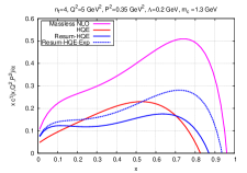
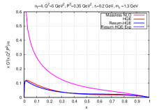
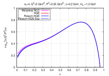
(a)	(b)	(c)

Figure 2: Parton distributions in the photon in ${\rm DIS}_{\gamma}$ scheme for $n_{f}=4$, $Q^{2}=5~{}$GeV², $P^{2}=0.35~{}$GeV² with $m_{c}=1.3~{}$GeV and $\Lambda=0.2~{}$GeV: (a) $xc^{\gamma}(x,Q^{2},P^{2})|_{{\rm DIS}_{\gamma}}$; (b) $xG^{\gamma}(x,Q^{2},P^{2})_{{\rm DIS}_{\gamma}}$, and the light singlet quark distribution (c) $xq^{\gamma}_{Ls}(x,Q^{2},P^{2})_{{\rm DIS}_{\gamma}}.$

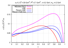
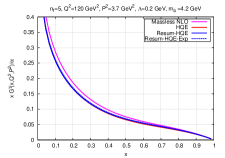
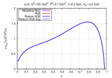
(a)	(b)	(c)

Figure 3: Parton distributions in the photon in ${\rm DIS}_{\gamma}$ scheme for $n_{f}=5$, $Q^{2}=120~{}$GeV², $P^{2}=3.7~{}$GeV² with $m_{b}=4.2~{}$GeV and $\Lambda=0.2~{}$GeV: (a) $xb^{\gamma}(x,Q^{2},P^{2})|_{{\rm DIS}_{\gamma}}$; (b) $xG^{\gamma}(x,Q^{2},P^{2})_{{\rm DIS}_{\gamma}}$, and the light singlet quark distribution (c) $xq^{\gamma}_{Ls}(x,Q^{2},P^{2})_{{\rm DIS}_{\gamma}}.$

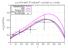
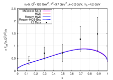
(a)	(b)

Figure 4: Effective structure functions for PLUTO (a); $n_{f}=4$, $Q^{2}=5~{}$GeV², $P^{2}=0.35~{}$GeV² with $m_{c}=1.3~{}$GeV and $\Lambda=0.2~{}$GeV: L3 (b) $n_{f}=5$, $Q^{2}=120~{}$GeV², $P^{2}=3.7~{}$GeV² with $m_{b}=4.2~{}$GeV and $\Lambda=0.2~{}$GeV.

V Conclusion

We have discussed the resummation of the heavy quark mass effects on the photon PDFs by changing the initial condition for the LO DGLAP equation. Our method is based on the mass-independent DGLAP evolution equation and a change of the initial condition for the heavy quark component in the LO solution of the DGLAP evolution equation.

We recovered the previous results based on the NLO OPE formalism KSUU2010 except for finite terms by taking a certain limit: $\ln(m^{2}/P^{2})\ll\ln(m^{2}/\Lambda^{2}$). By using the method, we can resum the large logarithmic terms due to heavy quark mass effects on photon PDFs in the virtual photon. We evaluate the size of the resummation effects numerically. The resummation effects for the charm quark PDF, gluon PDF are larger than that of the bottom quark PDF due to the heavy quark electromagnetic charge. We also see that the resummation of the heavy quark mass effects on the effective structure function tends to close to the experimental data in PLUTO case. Although we only presented the PDFs in the $\overline{\rm DIS}_{\gamma}$ scheme, the PDFs in the $\overline{\rm MS}$ scheme with our resummed heavy quark effects could be inferred from the difference between the PDFs in $\overline{\rm MS}$ and those in DIS_γ in our previous paper KSUU2010 where both schemes were explicitly presented.

Now some comments on the future extensions of the present work are in order. One of the possible extensions is the NLO analysis. We can solve the NLO DGLAP equation including the change of the initial condition for the LO DGLAP equation. Other possibility is the extension of this idea to the $n_{f}$ quarks system with two or more heavy quarks. In the case of two heavy flavours, this can be achieved by decomposing the $n_{f}$ quarks into the $n_{f}-2$ light quarks and two heavy quarks. Such an extension will be useful to analyse the virtual photon structure functions under the situation which contains both the massive bottom quark and the charm quark at Super KEK-B KEKB . Another example for the phenomenological application of this idea is to analyse the system with the heavy superpartners in the supersymmetric QCD.

Appendix A Summary of explicit expressions for the LO solution

We can obtain the expression with the heavy quark effects for $Ls,H,G,Lns$ components. Each elements of the LO solution is defined by

$$\mbox{\boldmath$q$}_{n}^{\gamma(0)}=\left(q_{Ls}^{(0),n}(t),~{}q_{H}^{(0),n}(t),~{}G^{(0),n}(t),~{}q_{Lns}^{(0),n}(t)\right).$$ (64)

Then the LO solutions are summarised as

$$q_{Ls}^{(0),n}(t)/\frac{\alpha}{8\pi\beta_{0}}$$ (65)

$$= \frac{4\pi}{\alpha_{s}(t)}\left[\frac{1}{1+d_{\psi}^{n}}\left(\frac{1}{n_{f}}K_{\psi}^{n}-K_{H}^{0,n}\right)\left(1-r^{d_{\psi}^{n}+1}\right)+\frac{n_{f}-1}{n_{f}}K_{\psi}^{0,n}\sum_{\pm}\frac{1}{1+d_{\pm}^{n}}\frac{\gamma_{\psi\psi}^{0,n}-\lambda_{\mp}^{n}}{\lambda_{\pm}^{n}-\lambda_{\mp}^{n}}\left(1-r^{d_{\pm}^{n}+1}\right)\right]$$

$$\hskip 19.91684pt+\left[-\frac{n_{f}-1}{n_{f}}r^{d_{\psi}^{n}}+\frac{n_{f}-1}{n_{f}}\sum_{\pm}\frac{\gamma_{\psi\psi}^{0,n}-\lambda_{\mp}^{n}}{\lambda_{\pm}^{n}-\lambda_{\mp}^{n}}r^{d_{\pm}^{n}}\right]\hat{q}_{H}^{(0),n}(0)/\frac{\alpha}{8\pi\beta_{0}},$$

$$q_{H}^{(0),n}(t)/\frac{\alpha}{8\pi\beta_{0}}$$ (66)

$$= \frac{4\pi}{\alpha_{s}(t)}\left[-\frac{1}{1+d_{\psi}^{n}}\left(\frac{1}{n_{f}}K_{\psi}^{n}-K_{H}^{0,n}\right)\left(1-r^{d_{\psi}^{n}+1}\right)+\frac{1}{n_{f}}K_{\psi}^{0,n}\sum_{\pm}\frac{1}{1+d_{\pm}^{n}}\frac{\gamma_{\psi\psi}^{0,n}-\lambda_{\mp}^{n}}{\lambda_{\pm}^{n}-\lambda_{\mp}^{n}}\left(1-r^{d_{\pm}^{n}+1}\right)\right]$$

$$\hskip 19.91684pt+\left[\frac{n_{f}-1}{n_{f}}r^{d_{\psi}^{n}}+\frac{1}{n_{f}}\sum_{\pm}\frac{\gamma_{\psi\psi}^{0,n}-\lambda_{\mp}^{n}}{\lambda_{\pm}^{n}-\lambda_{\mp}^{n}}r^{d_{\pm}^{n}}\right]\hat{q}_{H}^{(0),n}(0)/\frac{\alpha}{8\pi\beta_{0}},$$

$$G^{(0),n}(t)/\frac{\alpha}{8\pi\beta_{0}} = \frac{4\pi}{\alpha_{s}(t)}\left[K_{\psi}^{n}\sum_{\pm}\frac{1}{1+d_{\pm}^{n}}\frac{\gamma_{G\psi}^{0,n}}{\lambda_{\pm}^{n}-\lambda_{\mp}^{n}}\left(1-r^{d_{\pm}^{n}+1}\right)\right]+\sum_{\pm}\frac{\gamma_{G\psi}^{0,n}}{\lambda_{\pm}^{n}-\lambda_{\mp}^{n}}r^{d_{\pm}^{n}}\hat{q}_{H}^{(0),n}(0)/\frac{\alpha}{8\pi\beta_{0}},$$ (67)

$$q_{Lns}^{(0),n}(t)/\frac{\alpha}{8\pi\beta_{0}}=\frac{4\pi}{\alpha_{s}(t)}\frac{1}{1+d_{\psi}^{n}}K_{Lns}^{n}\left(1-r^{d_{\psi}^{n}+1}\right).$$ (68)

The first term of the above results corresponds to the massless result and the second term corresponds to the variation term due the resummed heavy quark mass effects. Note that there is no extra contribution due to the modification of the initial condition for the $Lns$ component. This is consistent with the result in our previous work KSUU2010 . These results are the new and main results in this paper.

References

• (1) http://lhc.web.cern.ch/lhc.
• (2) http://www.linearcollider.org/cms.
• (3) http://www-acc.kek.jp/kekb.
• (4) T. F. Walsh, Phys. Lett.  36 B (1971) 121; S. J. Brodsky, T. Kinoshita and H. Terazawa, Phys. Rev. Lett.  27 (1971) 280.
• (5) M. Krawczyk, A. Zembrzuski and M. Staszel, Phys. Rept.  345 (2001) 265; R. Nisius, Phys. Rept.  332 (2000) 165; M. Klasen, Rev. Mod. Phys.  74 (2002) 1221; I. Schienbein, Ann. Phys.  301 (2002) 128; R. M. Godbole, Nucl. Phys. Proc. Suppl.  126 (2004) 414.
• (6) T. F. Walsh and P. M. Zerwas, Phys. Lett.  44 B (1973) 195; R. L. Kingsley, Nucl. Phys.  B 60 (1973) 45.
• (7) N. Christ, B. Hasslacher and A. H. Mueller, Phys. Rev.  D 6 (1972) 3543.
• (8) E. Witten, Nucl. Phys.  B 120 (1977) 189.
• (9) W. A. Bardeen and A. J. Buras, Phys. Rev.  D 20 (1979) 166; 21 (1980) 2041(E).
• (10) G. Altarelli, Phys. Rep.  81 (1982) 1.
• (11) R. J. DeWitt, L. M. Jones, J. D. Sullivan, D. E. Willen and H. W. Wyld, Jr., Phys. Rev.  D 19 (1979) 2046; D 20 (1979) 1751(E).
• (12) M. Glück and E. Reya, Phys. Rev.  D 28 (1983) 2749.
• (13) S. Moch, J. A. M. Vermaseren and A. Vogt, Nucl. Phys.  B 621 (2002) 413.
• (14) A. Vogt, S. Moch and J. Vermaseren, Acta. Phys. Polon.  B 37 (2004) 683.
• (15) K. Sasaki, Phys. Rev.  D 22 (1980) 2143; Prog. Theor. Phys. Suppl.  77 (1983) 197.
• (16) M. Stratmann and W. Vogelsang, Phys. Lett.  B 386 (1996) 370.
• (17) M. Glück, E. Reya and C. Sieg, Phys. Lett.  B 503 (2001) 285; Eur. Phys. J.  C 20 (2001) 271.
• (18) T. Uematsu and T. F. Walsh, Phys. Lett.  101 B (1981) 263.
• (19) T. Uematsu and T. F. Walsh, Nucl. Phys.  B 199 (1982) 93.
• (20) G. Rossi, Phys. Rev.  D 29 (1984) 852.
• (21) F. M. Borzumati and G. A. Schuler, Z. Phys.  C 58 (1993) 139.
• (22) J. Chýla, Phys. Lett.  B 488 (2000) 289.
• (23) S. Moch, J. A. M. Vermaseren and A. Vogt, Nucl. Phys.  B 688 (2004) 101.
• (24) A. Vogt, S. Moch and J. A. M. Vermaseren, Nucl. Phys.  B 691 (2004) 129.
• (25) T. Ueda, K. Sasaki and T. Uematsu, Phys. Rev.  D 75 (2007) 114009.
• (26) Y. Kitadono, K. Sasaki, T. Ueda and T. Uematsu, Phys. Rev.  D 77 (2008) 054019.
• (27) K. Sasaki and T. Uematsu, Phys. Rev.  D 59 (1999) 114011.
• (28) H. Baba, K. Sasaki and T. Uematsu, Phys. Rev.  D 65 (2002) 114018.
• (29) K. Sasaki, T. Ueda and T. Uematsu, Phys. Rev.  D 73 (2006) 094024.
• (30) M. Drees and R. M. Godbole, Phys. Rev.  D 50 (1994) 3124.
• (31) M. Glück, E. Reya and M. Stratmann, Phys. Rev.  D 51 (1995) 3220; Phys. Rev.  D 54 (1996) 5515.
• (32) M. Fontannaz, Eur. Phys. J.  C 38 (2004) 297.
• (33) K. Sasaki and T. Uematsu, Phys. Lett.  B 473 (2000) 309; Eur. Phys. J.  C 20 (2001) 283.
• (34) T. Ueda, K. Sasaki and T. Uematsu, Eur. Phys. J.  C 62 (2009) 467.
• (35) M. Buza, Y. Matiounine, J. Smith, R. Migneron and W. L. van Neerven, Nucl. Phys.  B 472 (1996) 611;
I. Birenbaum, J. Blümlein and S. Klein, Nucl. Phys.  B 780 (2007) 40; 820 (2009) 417.
• (36) P. Aurenche, M. Fontannaz and J. Ph. Guillet, Z. Phys. C 64 (1994) 621; Eur. Phys. J.  C 44 (2005) 395.
• (37) M. Glück, E. Reya and I. Schienbein, Phys. Rev.  D 60 (1999) 054019; D 62 (2000) 019902(E); Phys. Rev.  D 63 (2001) 074008.
• (38) K. Sasaki, J. Soffer and T. Uematsu, Phys. Rev.  D 66 (2002) 034014.
• (39) F. Cornet, P. Jankowski, M. Krawczyk and A. Lorca, Phys. Rev.  D 68 (2003) 014010.
• (40) F. Cornet, P. Jankowski and M. Krawczyk, Phys. Rev.  D 70 (2004) 093004.
• (41) M. Glück, E. Reya and A. Vogt, Phys. Rev.  D 46 (1992) 1973.
• (42) Y. Kitadono, K. Sasaki, T. Ueda and T. Uematsu, Prog. Theor. Phys.  121 (2009) 495.
• (43) Y. Kitadono, K. Sasaki, T. Ueda and T. Uematsu, Phys. Rev.  D 81 (2010) 074029.
• (44) W. Furmanski and R. Petronzio, Z. Phys.  C 11 (1982) 293.
• (45) Ch. Berger et al. (PLUTO Collaboration), Phys. Lett.  B 142 (1984) 119.
• (46) M. Acciarri et al. (L3 Collaboration), Phys. Lett.  B 483 (2000) 373.
• (47) M. Glück, E. Reya and A. Vogt, Phys. Rev.  D 45 (1992) 3986.