A Search for Neutron Star Precession and Interstellar Magnetic Field Variations via Multiepoch Pulsar Polarimetry

Abstract

In order to study precession and interstellar magnetic field variations, we measured the polarized position angle of 81 pulsars at several-month intervals for four years. We show that the uncertainties in a single-epoch measurement of position angle is usually dominated by random pulse-to-pulse jitter of the polarized subpulses. Even with these uncertainties, we find that the position angle variations in 19 pulsars are significantly better fitted (at the 3$\sigma$ level) by a sinusoid than by a constant. Such variations could be caused by precession, which would then indicate periods of $\sim(200-1300)$ d and amplitudes of $\sim(1-12)$ degrees. We narrow this collection to four pulsars that show the most convincing evidence of sinusoidal variation in position angle.Also, in a handful of pulsars, single discrepant position angle measurements are observed which may result from the line of sight passing across a discrete ionized, magnetized structure. We calculate the standard deviation of position angle measurements from the mean for each pulsar, and relate these to limits on precession and interstellar magnetic field variations.

1 Introduction

Many pulsars are among the most highly polarized astrophysical sources of radiation. One polarized parameter, the position angle of linear polarization $\psi$ (also called the PPA – polarized position angle) is a particularly useful quantity: it carries information about the intrinsic geometry of the emitting region at the pulsar [e.g., via the rotating vector model (Radhakrishnan & Cooke, 1969)]; it also probes the magnetized plasma along the line of sight through Faraday rotation measurements [e.g., Weisberg et al. (2004)]. The purpose of this paper is to study the behavior of the polarized position angle on timescales of $10^{2-3}$ d, in order to investigate time-variable behaviors of pulsars’ magnetospheric geometry and the interstellar medium. For example, precession of the neutron star or other long-timescale oscillatory behavior affecting the emission beam will change the PPA, as will variations in the magnetized interstellar plasma along the line of sight.

2 Observations and Analyses

Ninety-eight pulsars were observed at 21 cm from Arecibo Observatory every few months for several years from 1989 to 1993. The resulting grand average polarized pulse profiles were analyzed in Weisberg et al. (1999), where observing details can also be found. In the present work, we found that we had adequate data on eighty-one of the pulsars to search for temporal variations of polarized position angle. For all of them, the polarized position angles were originally measured relative to an unknown origin. Consequently, in the present work, in order to search for temporal changes in position angle, we needed to reference our data to a position-angle standard. To do so, we selected two calibrator pulsars, B0540+23 (J0543+2329) and B1929+10 (J1932+1059). The calibrators were chosen on the basis of the relative constancy of their PPA’s during full-sky Arecibo observing tracks. We then compared the measured polarized position angle of a target pulsar on a given observing session to the PPA of one of the two calibrator pulsars. While the absolute position angle is still unknown, this referencing procedure enables us to be sensitive to position angle changes over time, assuming only that the position angle of the calibrators remains fixed over time. The procedures are described in the following sections; mathematical details are given in Appendix A.

In the rare cases where a calibrator pulsar was not observed during a daily session, we created an artificial “meshed” calibrator pulsar by determining its expected position angle on that session from observations of all other pulsars during that session.

2.1 A Pulsar’s Polarized Position Angle Curve

Pulsars tend to be very highly linearly polarized objects. The observed linear polarization originates at or near the star, often following the magnetic field lines at the point of origin (Radhakrishnan & Cooke, 1969), and is then modified by various propagation effects. We define the generic polarized position angle “curve ” for a pulsar at epoch $t$, a function of pulsar longitude $\phi$ at fixed $t$, as the set of polarized position angles $\psi(\phi,t)$ for $0\leq\phi\leq 2\pi$. (See the bottom panels of Fig. 2 for examples of PPA curves.)

The measured PPA curve at epoch $t$ can be expressed as the sum of five terms – an ensemble average (denoted below by angular brackets) for the indicated pulsar longitude $\phi$ and epoch $t$ which reflects the pulsar’s intrinsic orientation, an interstellar Faraday rotation term, an instrumental origin, and a term arising from errors due to radiometer noise and one from intrinsic pulse-to-pulse fluctuations in amplitude and phase of individual pulses (called “jitter;” see Cordes (1993) and further discussion below):

$$\psi(\phi,t)=\langle\psi(\phi,t)\rangle+\psi_{Faraday}(t)+\psi_{instr}(t)+\delta\psi_{noise}(\phi,t)+\delta\psi_{jitter}(\phi,t).$$ (1)

The first two terms on the right-hand side of the above equation hold the physics of interest in this experiment – namely the temporal behavior of the pulsar’s orientation or magnetosphere, and of the interstellar magnetic field through which its signals propagate, respectively. The third term defines the instrumentally measured PPA corresponding to an absolute PPA on the sky of zero. The latter two terms, though having zero mean, represent phenomena that add variance to the measurements, thereby limiting our precision in specifying the first two. We now discuss each of these five terms in order.

2.1.1 Variations in PPA Due to Changes in Orientation of the Pulsar or its Magnetosphere

(a) Precession: Precession would lead to a periodic wobble of the pulsar orientation. Most pulsar magnetospheric models indicate that the polarized emission is tied fundamentally to the geometry of the magnetic field in the emitting regions. Hence it is expected that a periodic wobble in pulsar orientation translates directly into a periodic variation of similar amplitude in polarized position angle. Therefore, a search for temporal variations in PPA is a sensitive probe for the presence of precession.

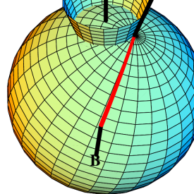
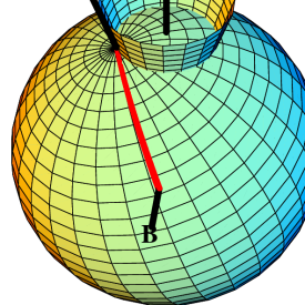
Figure 1: Two panels from the animation starPrecession.mpg, which is available at this link. Each panel of the animation shows a precessing pulsar stroboscopically at times (separated by multiples of $\sim$ 1 rotational period) that its beam points most directly at the observer; i.e., at those times when it is observable. The total angular momentum vector, $\bf{L}$, is conserved, while the body symmetry axis $\bf{k}$ describes a cone about $\bf{L}$ approximately once per spin period. The absence of perfect synchronization between these two rates leads to a slow apparent precession of $\bf{k}$ at successive observer viewing times. The above two panels from the animation were chosen to illustrate the pulsar geometry at the extrema of its precessional excursion. The beam / magnetic axis is $\bf{B}$. Note the changing orientation of the red meridian connecting $\bf{k}$ and $\bf{B}$ on precessional timescales. This meridian represents a fiducial magnetic field line projected onto the surface. In most pulsar models, linearly polarized emission will be oriented along (or perpendicular to) this meridian, so the precessional motion leads to a changing polarized position angle (PPA) on precessional timescales.

The simplest model is one where the wobble would result from the free precession of an asymmetric isolated pulsar, although there also exist models where the precession is forced by an external disk or companion (Qiao et al., 2003), or by the star’s own radiation (Melatos, 2000). We assume that the neutron star is approximately spherical, with a slight axially symmetric oblateness about a symmetry axis. Hence the three moments of inertia have the relationship $I_{1}\equiv I_{||}\gtrsim I_{2}=I_{3}$, where $I_{||}$ is the moment parallel to the symmetry axis. (For extension of the precession model to a triaxial body, see Akgün, Link, & Wasserman (2006)). Shaham (1986) and Jones & Andersson (2001) show that the motion of a point on the star can be decomposed into a quick rotation about the total angular momentum vector plus a slow precession about the body symmetry axis. For a sketch of the process and a link to an animation, see Fig. 1; for readers wishing to modify the geometrical parameters of the animation, the Mathematica source code is also available online at the Mathsource library (Everett & Weisberg, 2007). The angle $\theta$ between the angular momentum vector and symmetry axis leads to a “wobble” at both the rotation and precession frequencies, with the latter leading directly to a change in PPA of similar amplitude on precession timescales. Very slow precession, with a period of many years, would produce just a linear trend in PPA with epoch.

(b)Magnetospheric Adjustments: As we will describe below, there are theoretical difficulties (though not insoluble ones) with the picture of precession-induced pulse shape variations, centered primarily on the long observed timescales and relatively large inferred amplitudes. Ruderman & Gil (2006) have proposed an alternate model whereby the pulse shape and timing variations are caused by slowly rotating magnetospheric currents rather than by precession of the whole star. While this is an interesting alternative interpretation of the observations, more work needs to be done to flesh out the model and to verify that it can explain the observed timescales and amplitudes.

2.1.2 Variations in PPA Due to Changes in Interstellar Faraday Rotation

In this section, we focus on studying variations in the magnetized ISM plasma via a search for temporal variations in PPA. The second term of Eq. 1 quantifies Faraday rotation of the PPA in the interstellar medium, $\psi_{Faraday}(t)$, at some epoch, $t$. The rotation measure, $RM(t)$, is defined so as to specify the angle of PPA Faraday rotation at wavelength $\lambda$:

$$\psi_{Faraday}(t)=\lambda^{2}RM(t),$$ (2)

with angle in radians, $\lambda$ in m, and $RM(t)$ in rad m^-2.

A measured change in PPA, $\Delta\psi_{Faraday}$, then implies a change in Faraday rotation measure, $\Delta RM$:

$$\Delta RM=\frac{\Delta\psi_{Faraday}}{\lambda^{2}}.$$ (3)

In order to relate $\Delta RM$ to the ISM, we express $RM$ as a function of fundamental properties along the pulsar–Earth path:

$$RM=0.81\int_{0}^{D}B_{||}(s)\ n_{e}(s)\ ds,$$ (4)

where $B_{||}$ is the magnetic field parallel to the line of sight in $\mu$G, $n_{e}$ is the electron density in electrons cm^-3, and $ds$ is a differential path element whose integrated distance is $D$ (Lyne & Graham-Smith, 2006).

Each of the variables in Eq. 4 may be a function of time. While this time-variability could result directly from temporal changes in the ISM, it would more likely be induced by the pulsar’s motion rapidly sweeping the line of sight across a presumed spatially inhomogeneous ISM.

Since measurements show that temporal variations of dispersion measure $DM=\int_{0}^{D}{n_{e}ds}$, are generally quite small (Phillips & Wolszczan, 1991; Backer et al., 1993; Hobbs et al., 2004b; Weisberg et al., 2004; Ahuja, Gupta, & Kembhavi, 2005; You et al., 2007), we further expect that any observed variations in $RM$ would originate principally from the pulsar carrying the line of sight across an inhomogeneity in $B_{||}$. Therefore, we model the RM change as resulting from the line of sight passing across a discrete region having a variation in the parallel field, $\Delta B_{||}$, occupying a fraction $f$ of the pulsar-Earth path, with no associated $n_{e}$ variation.

In this case, $\Delta RM$, the $RM$ change due to the discrete region is

$$\Delta RM=0.81\int_{0}^{fD}\Delta B_{||}\ n_{e}ds\approx 0.81\ \Delta B_{||}\ f\ DM.$$ (5)

Finally, we can relate an observed change in PPA, $\Delta\psi_{Faraday}$, to the properties of the discrete region by combining Eqs. 3 and 5:

$$f\ \Delta B_{||}\approx\frac{\Delta RM}{0.81\ DM}=\frac{\Delta\psi_{Faraday}}{0.81\ \lambda^{2}\ DM};$$ (6)

or, expressed as a fractional variation:

$$\frac{f\ \Delta B_{||}}{\langle B_{||}\rangle}\approx\frac{\Delta RM}{RM}=\frac{\Delta\psi_{Faraday}}{\lambda^{2}RM},$$ (7)

where $\langle B_{||}\rangle$ is the line of sight average.

2.1.3 The Instrumental PPA and its Variance

The third term in Eq. 1 represents a conversion of absolute PPA on the sky, to PPA measured in the instrumental frame. The instrumental frame involves geometrical terms associated with telescope orientation as well as instrumental phase delays during a given session. As noted above in §2, we did not directly determine the instrumental PPA but rather referenced our measured PPA to the PPA of a calibrator pulsar, which has its own variance (see §2.2).

2.1.4 The Variance in PPA due to Radiometer Noise

The noise term in Eq. 1 results from the finite sampling statistics of a noisy signal and is familiar to all radioastronomers. Its contribution to the variance, $\sigma^{2}_{\psi,\rm\ noise}$, was determined empirically by measuring the variance off-pulse.

2.1.5 The Variance in PPA due to Pulse Jitter

The jitter term in Eq. 1 is unique to pulsars and requires further explanation, especially because it often dominates the error budget. We characterize as “jitter” all PPA changes on pulse-to-pulse timescales that are counterparts to the arrival-time jitter of individual subpulses. These random PPA variations occur due to various propagation effects in the pulsar magnetosphere analogous to Faraday rotation. These fluctuations might be correlated, for example, for the duration of a single subpulse in a given pulse period, but would be uncorrelated between subpulses and across pulse periods. Random variations in altitude of emission would produce a PPA curve that is shifted earlier or later for higher or lower altitudes, respectively. This kind of variation would also be highly correlated across a single subpulse. The variance of $\psi$ due to jitter, $\sigma^{2}_{\psi,\rm\ jitter}$, is calculated as follows.

By definition, uncertainties $\sigma_{I,\rm\ jitter}(\phi)$ and $\sigma_{L,\rm\ jitter}(\phi)$ in polarized parameters $I(\phi)$ (total power at longitude bin $\phi$) and $L$ (linearly polarized power at longitude bin $\phi$) due to random pulse-to-pulse jitter are characterized by

$$\sigma_{I,\rm\ jitter}(\phi)\equiv m_{I}(\phi)I(\phi),$$ (8)

and

$$\sigma_{L,\rm\ jitter}(\phi)\equiv m_{L}(\phi)L(\phi),$$ (9)

where $m_{X}$ is the “modulation index” of polarized parameter $X$, a measure of its pulse-to-pulse modulation.

In our experiment, each polarized profile was integrated online for two minutes, thereby attenuating these pulse-to-pulse modulations. Therefore, the jitter-induced fluctuations in the measurement of these quantities after $N$ pulses, will be

$$\sigma_{I,\rm\ jitter}(\phi,N)=\sigma_{I,\rm\ jitter}(\phi)/\sqrt{N}=m_{I}(\phi)I(\phi)/\sqrt{N},$$ (10)

and

$$\sigma_{L,\rm\ jitter}(\phi,N)=\sigma_{L,\rm\ jitter}(\phi)/\sqrt{N}=m_{L}(\phi)L(\phi)/\sqrt{N}.$$ (11)

At high $S/N$ and under the reasonable assumption that $\sigma_{Q}\approx\sigma_{U}$, $\sigma_{L}$ propagates to an uncertainty in position angle $\sigma_{\psi}$:

$$\sigma_{\psi}(\phi)\approx\sigma_{L}(\phi)/(2L(\phi))$$ (12)

(Naghizadeh-Khouei & Clarke, 1993). Therefore, the jitter-induced uncertainty in the measurement of PPA in an integration of $N$ pulses is

$$\sigma_{\psi,\rm jitter}(\phi,N)\approx m_{L}(\phi)/(2\sqrt{N})$$ (13)

As we shall see below in §2.2, we must ultimately determine $\sigma_{\psi,\rm jitter}$, the jitter-induced fluctuation in the PPA integrated not only over $N$ pulses but also over the full range of longitudes. With the subpulse as the basic unit of correlated emission, the jitter-induced fluctuations in the measurement of PPA after $N$ pulses, each containing $n$ subpulses, will be characterized by

$$\sigma_{\psi,\rm jitter}=\sigma_{\psi,\rm jitter}(N,n)=\sigma_{\psi,\rm jitter}(\phi,N)/\sqrt{n}\approx m_{L}/(2\sqrt{Nn}).$$ (14)

Since we could not directly measure the quantities $m_{L}$ and $n$ with our two-minute integrations, we surveyed the literature for typical values. Many observations suggest that $m_{I}\sim 1$ (Bartel et al., 1980; Weisberg et al., 1986; Weltevrede et al., 2006) and the few extant polarized modulation index observations (e.g., Jenet, Anderson, & Prince (2001)) support the reasonable assumption that $m_{L}\sim 1$ as well. Single-pulse observations indicate that $n$ is also approximately 1. Finally, we found that constant-$\psi$ fits to the full set of pulsars had a mean $\chi_{\nu}^{2}\sim 1$ when $m_{L}/\sqrt{n}\sim 1.7$ in Eq. 14, so we adopted this value; i.e.,

$$\sigma_{\psi,jitter}\sim 0.85/\sqrt{N}.$$ (15)

We empirically tested the relative contributions of radiometer noise and pulse jitter to the PPA uncertainty in the following tests on one of the two calibrator pulsars, B0540+23. We observed it for several $\sim$two-hour stretches with a series of standard two-minute integrations identical in form to all others in this experiment, and analyzed the resulting data as follows. First, a linear trend in PPA, presumably due to variable ionospheric Faraday rotation, was fitted and subtracted out . For PSR B0540+23, the uncertainty in PPA resulting from radiometer noise was $\sigma_{\psi,\rm noise}\sim 0\fdg 2$, while the observed standard deviation of two-minute integrations from the linear trend was a far larger $\sim 1\arcdeg$. Pulse jitter considerations, however, lead via Eq. 15 to an estimated $\sigma_{\psi,\rm jitter}\sim 2\arcdeg$.

While the jitter uncertainty estimated via Eq. 15 appears to be about twice the observed standard deviation, it is important to bear in mind that the simplifying assumptions used in the jitter calculation can easily lead to factor of $\sim 2$ errors in either direction for a particular pulsar, as they apparently have in this case. (See further discussion in §3.2). Nevertheless, the important conclusion of this exercise is that the actual PPA uncertainty is far larger than that due to radiometer noise alone, and that pulse jitter appears to be the predominant source of the observed noise, with an amplitude in rough agreement with our model. Note also that the jitter model should give excellent results for a given pulsar if all factors in Eq. 14 are directly measured, rather than using an average over our pulsar sample, as in Eq. 15.

2.2 Estimation of a Pulsar’s Polarized Position Angle Offset with Respect to a Calibrator Pulsar, and its Variance

In order to study temporal variations in a pulsar’s orientation or in the intervening medium, we investigate the PPA as a function of time. As noted in §2 , the instrumental PPA origin, $\psi_{instr}(t)$ of Eq. 1, was not explicitly measured. Instead, we reference our target pulsar PPA’s to “calibrator” pulsars B0540+23 or B1929+10, which can be considered PPA “beacons” of constant but unknown PPA. We do so in a three-step process: first we find the offset of the target pulsar’s PPA curve at epoch $t$ from a high $S/N$ “template” PPA curve of the same pulsar from Weisberg et al. (1999) (see Fig. 2a and Eq. A1). Next we do the same procedure at the same epoch on the calibrator pulsar B0540 or B1929+10 (see Fig. 2b and Eq. A2). Finally, to yield the desired offset of the target pulsar from the calibrator pulsar at epoch $t$, $\Delta\psi(t)$, we difference the above two results (see Eq. A3).

The variance in a target pulsar-template PPA difference measurement, $\sigma^{2}_{\psi(t)}$, is the sum of the noise and jitter contributions from the target pulsar at epoch $t$ (the template contributes negligibly):

$$\sigma_{\psi(t)}^{2}=\sigma_{\psi(t),\rm\ noise}^{2}+\sigma_{\psi(t),\rm\ jitter}^{2}.$$ (16)

A similar equation holds for the variance in a calibrator pulsar-template PPA difference measurement, $\sigma^{2}_{\psi_{\rm{cal}}(t)}$. However, we are ultimately interested in the variance of the position angle of a pulsar with respect to the calibrator pulsar, (cf. Eq. A3). This variance, $\sigma^{2}_{\Delta\psi(t)}$, will then be the sum of the above-discussed variances in the pulsar-template and calibrator-template PPA difference measurements:

$$\sigma_{\Delta\psi(t)}^{2}=\sigma_{\psi(t)}^{2}+\sigma_{\psi_{cal}(t)}^{2}.$$ (17)

3 Results

We searched for evidence of temporal variations of polarized position angle in each of the 81 target pulsars, with an emphasis on a few likely signatures: (1) sinusoidal variations in PPA due to periodic phenomena at the pulsar such as precession, as described in §2.1.1; (2) discontinuous changes in PPA caused by interstellar propagation effects, such as the line of sight crossing a region with significantly different magnetic field, as discussed in §2.1.2; and (3) ramps in PPA caused by phenomena such as those listed above, having a characteristic time longer than our experiment’s. For each pulsar, the dataset consists of the measured PPA offsets, $\Delta\psi(t)$ (cf. Eq. A3) , and their estimated uncertainties, $\sigma_{\Delta\psi(t)}$ (cf. Eq. 17), at a set of epochs, $t$. In the following sections, we give an overview of these results. See the Discussion (§4) for exploration of the astrophysical implications.

3.1 Sinusoidal Variations of Polarized Position Angle

To test for possible periodic variations in each pulsar’s PPA, we fit a sine function to $\Delta\psi(t)$. This sine function requires four free parameters: the zero-point $\Delta\psi_{\rm 0}$ about which the sinusoid oscillates; the amplitude $a_{\psi}$ of the sinusoid about $\Delta\psi_{\rm 0}$; the period $P_{\psi}$ of the sinusoid; and a phase offset $t_{0}$:

$$\Delta\psi(t)=\Delta\psi_{0}+a_{\psi}\sin[2\pi(t-t_{0})/P_{\psi}].$$ (18)

In fitting with these free parameters, we had two chief concerns: that our best-fit results for this function’s parameters not be dependent on initial guesses for those parameters, and that we only accept the sinusoidal fit’s results when that fit represents a statistically significant improvement over the fit of a constant, $\overline{\Delta\psi}$.

To ensure that the fit results were not dependent on initial guesses, we ran trial fits on a large number of initial values for both sinusoidal period $P_{\psi}$ and amplitude $a_{\psi}$. The initial-parameter search space for the amplitude was set to lie in the interval [$0^{\circ},2\cdot\rm{max}(\Delta\psi(t)-\overline{\Delta\psi})$]. Meanwhile, the maximum sinusoidal period was set to $5\cdot\Delta t$, where $\Delta t$ is the total timespan of the observations, in order to look for long-timescale variations. The minimum sinusoidal period tested was to $2\cdot\Delta t/N_{\rm sessions}$ where $N_{\rm sessions}$ is the number of observation sessions for each pulsar. This range of sinusoidal amplitude and period was then used to define a linearly-spaced grid of $501\times 501$ initial guesses. A separate non-linear least-squares fit was run for each set of initial parameters, where all four parameters were allowed to “float” freely; the only exception to this was that the period was not allowed to fall below the minimum period already defined. Of all of the resultant converged fits, the sinusoid with the minimum $\chi^{2}$ was selected as the best fit for that pulsar. As a final check, we re-ran the analysis with a $4001\times 4001$ grid of initial guesses; no significant changes to our fit results were found.

To check that the best sinusoidal model significantly improves the fit when compared to the constant-PPA model, we applied the F-Test (see §11.4, Bevington & Robinson, 1992). For the best-fit sinusoid for each pulsar, we calculated the $F_{\chi}$ statistic, where $F_{\chi}=\Delta\chi^{2}/\chi^{2}_{\nu}$. Here, $\Delta\chi^{2}$ is the difference in $\chi^{2}$ between the best-fit constant PPA and the best-fit sinusoid, and $\chi^{2}_{\nu}$ is the reduced $\chi^{2}$ value for the best-fit sinusoid. To assess its significance, one calculates the probability that the sinusoidal model’s improved fit would be achieved with random data. To accept it as formally significant, we ask that the sinusoidal fit be an improvement over the constant-PPA fit at the $P\sim 99.7\%$ level (approximately $3\sigma$); i.e., we require that the calculated improvement in $\chi^{2}$ would be less than $\sim 0.3\%$ probable, given a random sample of data points.

We find that nineteen of our pulsars meet or exceed this sinusoidal vs. constant-PPA F-Test significance level, indicating statistically significant sinusoidal PPA variations with time. It is important, however, to recognize that a particular pulsar’s F-Test significance calculation is only advisory, given the uncertainty in the value of the pulse jitter variance (see §2.1.5), which enters crucially as a scale factor in the reduced $\chi^{2}$ calculation. Nevertheless, there is a clear pattern of statistically significant improvement in many fits across our pulsar sample when a sinusoidal model is introduced. The details of the nineteen pulsars’ statistically significant fits, along with two additional ones (see below), are listed in Table 1.

To highlight our assessment of the quality of the fits, we group the 81 sinusoidal fits into four different classes (see Table 1 for designations of all pulsars in the three highest classes). The top two classes have formally significant ($P\gtrsim 0.997$) fits, while the bottom two do not. “Class I” pulsars are those whose sinusoidal fits we find particularly convincing. The data and fits for these four pulsars are shown in Fig. 3. “Class II” consists of those pulsars where we find the fit less convincing, although still formally significant, for two principal reasons. (i) If there is a large spread in the PPA values that seems to not be accounted for by the sinusoid, possibly indicating non-sinusoidal variation in the PPA (see an example in Fig. 4); or (ii) if the constant-PPA fit itself appears sufficient $(\chi_{\nu}^{2}\mathrel{\hbox{\hbox to0.0pt{\hbox{\lower 4.0pt\hbox{$\sim$}}\hss}\hbox{$<$}}}1)$, therefore calling into question the need for a sinusoid. “Class III” pulsars are those that we judge might have sinusoidal variation, although the fit was not a formally significant improvement over the constant-PPA fit. Both such pulsars’ fits are displayed in Fig. 5. “Class IV” encompasses the remaining 60 pulsars, which have neither formal nor apparent sinusoidal tendencies. See Figure 6 for an example.

3.1.1 Ultralong-Period Variations in Polarized Position Angle

In our sinusoidal fits (cf. §3.1), none of the trial fits with long-period variations (longer than the total timespan of observations) is a significant improvement over the constant PPA fit at the $3\sigma$ level. Therefore, there is no evidence in our data of variations in PPA, including ramps, on these ultralong timescales. See §3.2 for a discussion of upper limits on PPA variations from a (constant) mean on shorter timescales.

3.2 Upper Limits on Temporal Variations from the Mean Polarized Position Angle

Table A Search for Neutron Star Precession and Interstellar Magnetic Field Variations via Multiepoch Pulsar Polarimetry presents a full summary of our PPA versus time measurements for the 81 pulsars. The table is organized into three principal categories. (i) Pulsar Details: The first seven entries for a given pulsar list catalog information such as pulsar name and $DM$ and $RM$; (ii) Data Catalog: The next four entries detail our observations, listing total timespan, total number of sessions, and the number rejected due to the PPA being many $\sigma_{\Delta\psi(t)}$ from the mean (see §3.2.1 for further details on the rejects); and (iii) Retained Session Results: These results represent important upper limits derived from the “sessions retained” after the editing process, and are discussed further below.

The standard deviation of the position angle of a given pulsar, called $\sigma_{\psi}$ in the “Retained Session Results” section of Table A Search for Neutron Star Precession and Interstellar Magnetic Field Variations via Multiepoch Pulsar Polarimetry, is one of the most important quantities measured in this experiment. It represents the typical deviation of any single PPA measurement from the mean position angle. (For the pulsars exhibiting possible sinusoidal variations, the standard deviation from the sinusoid, $\sigma_{\psi,\rm sine}$, is also presented in Table 1). Together, these results represent, to our knowledge, the only published systematic measurements of time variations (or their upper limits) of pulsar polarized position angles.

3.2.1 Discontinuous Changes in Polarized Position Angle

As noted in §3.2, there are a handful of measured $\Delta\psi(t)$ lying many $\sigma_{\Delta\psi(t)}$ away from the mean value for a given pulsar. (See the “Sessions Manually Rejected” column of Table A Search for Neutron Star Precession and Interstellar Magnetic Field Variations via Multiepoch Pulsar Polarimetry for a listing of the pulsars having “manually” rejected sessions, and Table 3 for details on these sessions’ properties.) There are only six such rejected sessions among all 81 pulsars, and never more than one per pulsar. We have examined the polarized profile in each such case and see no evidence for instrumental problems. These puzzling events, if real, indicate the passage of ionized, magnetized structures across the line of sight on timescales shorter than the several-month intervals between observing sessions.

4 Discussion

As noted above, polarized position angle variations could be caused either by phenomena at the pulsar (e.g., precession or magnetospheric adjustments in the emission beam geometry); or by interestellar Faraday rotation variability. The observed measurements and upper limits on position angle changes reported in Tables 1 - 3 can be translated (1) directly into changes or upper limits thereof in projected spin axis or magnetospheric orientation; or to (2) changes or upper limits thereof in interstellar magnetic fields via Faraday rotation. We now discuss each in turn.

4.1 Changes in Orientation of the Pulsar or its Magnetosphere

4.1.1 Precession or Pulsar Magnetospheric Changes

Much theoretical work suggests that the amplitude of the precession would be smaller than a degree, which would place it below the threshold of measurability for most pulsars in this experiment (cf. Table A Search for Neutron Star Precession and Interstellar Magnetic Field Variations via Multiepoch Pulsar Polarimetry), and furthermore that it would quickly damp, at least in the presence of rigid pinning or even the slow creep of superfluid vortices [e.g., Shaham (1977); Sedrakian et al. (1999); Link (2006)]. Nevertheless, there are several observations of periodic changes in pulse shape and/or in arrival times of isolated pulsars in the literature, along with ours, that seem to indicate the presence of precession. In a few of the other cases, the derived amplitude is on the order of one to several degrees and the period is in the few-yr range, which are similar to our results. The best documented example is PSR B1828-11, whose arrival times and pulse shape vary periodically and in a correlated fashion, indicating precession with a period on the order of 1 yr and $0\fdg 3$ amplitude (Stairs, Lyne, & Shemar, 2000), or $\sim 3\arcdeg$ (Link & Epstein, 2001; Rezania, 2003) or possibly more (Akgün, Link, & Wasserman, 2006). PSR B1642-03 also exhibits both phenomena (Cordes & Downs, 1985; Blaskiewicz, 1991), which have been modeled as stemming from precession with an amplitude of $0\fdg 5-0\fdg 8$ over several yr (Cordes, 1993; Shabanova, Lyne, & Urama, 2001).⁴ Suleymanova & Shitov (1994) discovered pulse shape and timing variations in PSR B2217+47, which they modeled as induced by precession with a timescale $\gtrsim 20$ yr. PSR B1557-50 shows a several-year timing and dispersion measure periodicity (the latter interpreted as possible frequency-dependent temporal pulse shape variations) which is modeled as precession with an amplitude of $\sim 0\fdg 01$ (Chukwude, Ubachukwu, & Okeke, 2003). D’Allesandro & McCulloch (1997) observed quasiperiodic timing and profile variations in PSR B0959-54 which could be caused by precession with a period $\gtrsim$ 2500 d and amplitude $\leq 0\fdg 15$. Quasiperiodicities on several hundred day timescales in Crab Nebula pulsar arrival times may also indicate precession (Lyne et al., 1988; Scott et al., 2003). Deshpande & McCulloch (1996) observed pulse shape, PPA, and timing variations in the Vela pulsar which they suggested could result from free precesssion with a 330-d period; and Deshpande & Radhakrishnan (2007) further elaborated the precession model to explain variations in X-ray morphology of the Vela Pulsar’s Pulsar Wind Nebula. Zhu & Xu (2006) have proposed that the Galactic Center Radio Transient GCRT J1745-3009 could be a neutron star precessing by $\gtrsim 15\arcdeg$, although an experiment like the current one would be insensitive to its 77-min period. Finally, the X-ray emitting isolated neutron star RX J0720.4-3125 exhibits a wide variety of correlated periodic phenomena indicative of precession on a 7-8 yr timescale (Haberl et al., 2006).

Our analysis shows that 19 of our 81 pulsars exhibit PPA variations that are significantly better fit (at approximately the 3$\sigma$ level) by a sinusoidal PPA function than by a constant PPA. Of these, we judge four pulsars to exhibit the most convincing evidence for sinusoidal variations in PPA. (These are our “Class I” pulsars: B0523+11, B0611+22, B0656+14, and B2053+21; see Fig. 3). Our results indicate that variations, and even sinusoidal variations, are occasionally present in the pulsar population. As a group, these 19 pulsars display sinusoidal periods mostly grouped around 185 to 450 days, with a peak at 200 days and outliers at approximately 790, 1050, and 1250 days. The amplitude of the variation ranges from 1^∘ to 8^∘ for most of the significant fits, with a peak at 2^∘ and an outlier at 12^∘. Note that these sinusoidal results do not include the six large PPA excursions, rejected from the fits in Table A Search for Neutron Star Precession and Interstellar Magnetic Field Variations via Multiepoch Pulsar Polarimetry and detailed in Table 3; as these large excursions do not carry the signature of precession even if they are real.

In §2.1.1b, we briefly discussed rotating magnetospheric currents as a possible source of periodic PPA changes. In the absence of well-developed models, we only note here that such phenomena might provide an alternate explanation for the observed periodic PPA variations.

4.2 Interstellar Magnetic Field Variations

Table 3 lists the properties of those few PPA measurements lying far from the mean. As noted above, these could indicate the presence of magnetized variations in the ISM, although they might conceivably result instead from an experimental problem. Under the first assumption (magnetized ISM variations causing the deviations), we calculate and list in Table 3 the quantities $\Delta RM(t)$ (Eq. 3) and $\Delta RM(t)/RM\approx f\Delta B_{||}(t)/\langle B_{||}\rangle$ (Eq. 7). However, the great majority of our pulsars shows no evidence whatsoever of PPA variations above the noise. Under the second assumption (that the few large PPA deviations observed are spurious), our measured upper limits on temporal variations of position angle among “Retained Sessions” (the quantity $\sigma_{\psi}$ of Table A Search for Neutron Star Precession and Interstellar Magnetic Field Variations via Multiepoch Pulsar Polarimetry) can be interpreted as upper limits on magnetized variations, again via Eqs. 3 and 7 where the quantities $\Delta\psi_{Faraday}$ and $\Delta RM$ are replaced by their respective statistical analogs, $\sigma_{\psi}$ and $\sigma_{RM}$. Table A Search for Neutron Star Precession and Interstellar Magnetic Field Variations via Multiepoch Pulsar Polarimetry lists these derived upper limits on $\sigma_{RM}$ and $\sigma_{RM}/RM\ (\approx f\sigma_{B_{||}}/\langle B_{||}\rangle$).

There are occasional reports in the literature of temporal variations in interstellar magnetic fields, some of which may have origins similar to ours. First, there are the cases of the Vela and Crab Nebula Pulsars (Hamilton et al., 1985; Rankin et al., 1988). The variations of $RM$ (and also of $DM$) are so large and frequent that they are almost certainly associated with passage of inhomogeneous nebular SNR material across the line of sight. This interpretation is easy to reconcile with these pulsars’ relative youth and the observed presence of an SNR. There are other reports in the literature of $RM$ variations toward ordinary pulsars on multiyear timescales, sometimes accompanied by $DM$ variations as well (van Ommen et al., 1997), which appear to be caused by the passage of a cloud across the line of sight. Weisberg et al. (2004) measured many pulsar $RM$s and compared their results with earlier work wherever possible. They noted numerous cases of $RM$s changing significantly with respect to values measured $\sim(5-20)$ yr earlier, while the $DM$ tended to vary far less on similar timescales.

Yet our sample of pulsars exhibits only rare evidence for $RM$ variations over the four years of observation, and no evidence for sustained changes or long-term trends. We can suggest several possible resolutions to the disagreement between the rather common $RM$ changes in the literature and our finding of essentially steady $RM$s in our sample: (1) $RM$ variations tend to be small on the four-year timescale of our experiment, but grow on decade-long scales. This would have interesting implications for the fluctuation spectrum of interstellar plasma. However, recall that we have some sensitivity to changes on timescales longer than our dataspan, but no evidence was found for variations on scales beyond $\sim 10^{3}$ d. (2) A subtle nonorthogonal emission mode competition process can lead to spurious apparent $RM$ variations (Ramachandran et al., 2004), which might grow with time. (3) One of the previously published multiepoch $RM$ measurements was incorrect. This latter possibility cannot be ruled out, since $RM$ measurements are difficult, and since the pairs of observations were frequently performed by different groups on different telescopes. Further measurements are required in order to determine the correct explanation.

5 Conclusions

We have studied the temporal behavior of polarized position angle in 81 pulsars over a $\sim 4$ yr period. We demonstrate that the intrinsic pulse-to-pulse jitter of polarized subpulses frequently dominates the uncertainty in position angle determination. We searched particularly for sinusoidal variations, discontinuous changes, and linear trends in the data. Nineteen pulsars have variations in PPA that were significantly better fit (at the 3$\sigma$ level) by a sinuoidal function than by a constant; such variations could be caused by precession or other cyclical phenomena at the pulsar. These pulsars (and especially the four pulsars in our “Class I”) are good candidates for further study. A handful of discontinuous changes were observed in the sample, which could be due to the passage of the line of sight across an interstellar region with significantly different magnetized properties. No linear variations (i.e., “ramps”) of PPA across the timespan of observations were detected. For all 81 pulsars, we also calculate upper limits on random variations of PPA from the mean, which provide numerical constraints on precession and magetized interstellar variations in our sample.

Appendix A Equations for Determination of a Target Pulsar’s PPA Offset with Respect to a Calibrator Pulsar

At an observing session at epoch $t$, we measure the position angle curves of target and calibrator pulsars as a function of longitude $\phi$, $\psi(\phi,t)$ and $\psi_{\rm cal}(\phi,t)$, respectively. The high $S/N$ position angle curves of Weisberg et al. (1999), which are coherent sums over all sessions, serve as templates against which to measure shifts in position angle for a given pulsar on a particular observing session. The position angle curve of these target and calibrator templates as a function of longitude $\phi$, is $\bar{\psi}(\phi)$ and $\bar{\psi}_{\rm cal}(\phi)$, respectively. (See Fig. 2 for examples of session and template position angle curves of a target and a calibrator pulsar).

We first determine $\psi(t)$, the target pulsar’s weighted, longitude-averaged difference between PPA at an observing session at epoch $t$ and PPA of its summed template (see Fig. 2a for a target pulsar’s session and template PPA curves):

$$\psi(t)=\frac{\sum_{r=1}^{R}{w(\phi)[\psi(\phi,t)-\bar{\psi}(\phi)}]}{\sum_{r=1}^{R}w(\phi)},$$ (A1)

where the summations are over $R$ longitude bins.

Similarly, we also determine $\psi_{\rm cal}(t)$, the calibrator pulsar’s weighted⁴, longitude-averaged difference between PPA at an observing session at epoch $t$ and PPA of its summed template (see Fig. 2b for a calibrator pulsar’s session and template PPA curves):

$$\psi_{\rm cal}(t)=\frac{\sum_{r=1}^{R}{w(\phi)[\psi_{\rm cal}(\phi,t)-\bar{\psi}_{\rm cal}(\phi)}]}{\sum_{r=1}^{R}w(\phi)}.$$ (A2)

Then the quantity of interest for this experiment, $\Delta\psi(t)$, the polarized position angle offset of the target pulsar with respect to a calibrator pulsar at epoch $t$, is:

$$\Delta\psi(t)=\psi(t)-\psi_{\rm cal}(t).$$ (A3)

Note then that the desired $\Delta\psi(t)$ of a target pulsar is ultimately determined via a double-differencing procedure on the various PPAs – first both the target and calibrator pulsars’ PPAs at epoch $t$ are differenced from their templates, as in Eqs. A1 and A2; and finally the resulting target and calibrator epoch-template differences are differenced from one another, cf. Eq. A3.

As pointed out in §2 (see also Eq. 1), all of the above measured position angles contain an unknown instrumental origin $\psi_{instr}(t)$. Note that care was taken to measure both the target and the calibrator pulsar with an identical instrumental configuration and hence identical instrumental origin throughout a session at some epoch $t$. Therefore $\psi_{instr}(t)$ drops out of Eq. A3 due to the differencing of two terms, each containing this quantity. As a result, temporal variations in PPA are accessible even if the absolute PPAs themselves are not.

Further, we focus on temporal changes by subtracting a weighted mean offset $\overline{\Delta\psi}$ for each pulsar, before plotting the final values $\Delta\hat{\psi}(t)$, where

$$\Delta\hat{\psi}(t)=\Delta\psi(t)-\overline{\Delta\psi}.$$ (A4)

and

$$\overline{\Delta\psi}=\frac{\sum w(t)\Delta\psi(t)}{\sum w(t)},$$ (A5)

with the summations being over all observing sessions. The horizontal solid line placed at $\Delta\hat{\psi}=0$ in Figs. 3 and 4 then delineates the mean measured position angle in the new coordinate system defined by Eq. A4. The error bar on each individual measurement is $\sigma_{\Delta\psi(t)}$, as discussed above in §2.2 and defined in Eq. 17.

Table 1: Best Sinusoidal Fits to Polarized Position Angle as a Function of Time

Pulsar			Const.		Sinusoidal PPA
PSR J	PSR B		PPA
			$\chi^{2}_{\nu}$		$\chi^{2}_{\nu}$	$P_{\rm min}$	$P_{\rm max,i}$	$P_{\rm best,i}$	Ampl.	$\sigma_{\psi,\rm sine}$	F-Test	Prob.	Class
						[d]	[d]	[d]	$a_{\psi}\ [\arcdeg]$	$[\arcdeg]$
J0525+1115	B0523+11		1.92		0.03	435	6532	1250	12.46	0.47	312.51	0.9968	I
J0614+2229	B0611+22		1.01		0.63	187	6546	313	2.14	1.17	10.73	0.9982	I
J0629+2415	B0626+24		0.63		0.14	228	5692	356	2.33	0.55	35.25	0.9997	II
J0659+1414	B0656+14		1.38		0.47	285	7120	1047	2.47	0.85	20.24	0.9985	I
J1136+1551	B1133+16		1.37		0.75	234	7603	364	2.81	1.47	12.97	0.9987	II
J1607–0032	B1604–00		3.95		0.48	324	5667	380	12.42	3.14	46.31	0.9948	III
J1740+1311	B1737+13		1.05		0.69	106	6615	185	2.97	1.80	15.94	1.0000	II
J1805+0306	B1802+03		1.98		1.70	114	7118	209	2.46	2.73	6.95	0.9980	II
J1823+0550	B1821+05		1.25		0.90	143	7129	206	4.62	2.92	10.40	0.9995	II
J1844+1454	B1842+14		0.60		0.36	158	7118	221	1.67	1.22	14.60	0.9999	II
J1857+0057	B1854+00		6.08		4.86	150	7129	270	7.67	7.21	7.54	0.9974	II
J1915+1009	B1913+10		0.41		0.25	190	7123	443	1.69	1.06	12.62	0.9993	II
J1916+0951	B1914+09		0.23		0.06	265	6634	454	1.92	0.59	27.47	0.9993	II
J1920+2650	B1918+26		2.25		0.26	345	5179	869	15.38	2.68	41.51	0.9764	III
J1932+2220	B1930+22		0.82		0.44	168	7126	787	1.92	1.23	16.91	0.9999	II
J1954+2923	B1952+29		0.83		0.39	158	7126	213	4.00	1.84	22.24	1.0000	II
J2022+2854	B2020+28		0.89		0.47	160	7604	176	4.21	1.57	18.84	1.0000	II
J2037+1942	B2034+19		0.75		0.49	186	6521	208	6.92	3.69	9.72	0.9974	II
J2055+2209	B2053+21		2.69		1.42	201	6521	444	5.75	3.29	13.78	0.9990	I
J2124+1407	B2122+13		2.13		1.24	186	6034	289	8.95	4.66	11.50	0.9980	II
J2212+2933	B2210+29		0.70		0.23	201	6045	310	3.65	1.29	26.25	0.9998	II

Table 2: Measured Parameters and Quanities Derived Assuming Constant PPA

Pulsar Details							Data Catalog				Retained Session Results
Name		DM		RM
							Time-	Total	Sessions	Ses-	$\sigma_{\psi}$	$\sigma_{RM}$	$\underline{\sigma_{RM}}$	Re-	Outliers
PSR J	PSR B	Value	Ref.	Value	$\pm$	Ref.	span	Ses-	Manually	sions			$|RM|$	duced	$>3\sigma$
		(pc/cm3)		(rad/m2)			(yr)	sions	Rejected	Retained	(deg)	(rad/m2)		$\chi^{2}$
J0304+1932	B0301+19	15.74	1	-8.30	0.30	6	3.6	13	0	13	1.49	0.59	0.071	0.6	0
J0525+1115	B0523+11	79.34	1	35.00	3.00	7	3.6	6	0	6	3.73	1.48	0.042	1.9	0
J0528+2200	B0525+21	50.94	1	-39.60	0.20	8	3.6	16	0	16	3.74	1.48	0.037	0.6	0
J0614+2229	B0611+22	96.91	1	69.00	2.00	6	3.6	14	0	14	1.75	0.69	0.010	1.0	0
J0629+2415	B0626+24	84.19	1	69.50	0.20	7	3.6	10	0	10	1.51	0.60	0.009	0.6	0
J0659+1414	B0656+14	13.98	1	23.50	0.40	7	3.9	10	0	10	1.88	0.74	0.032	1.4	0
J0754+3231	B0751+32	39.95	1	-7.00	5.00	9	3.9	11	0	11	4.06	1.61	0.230	1.8	1
J0826+2637	B0823+26	19.45	1	5.90	0.30	6	3.9	8	0	8	1.56	0.62	0.105	0.6	0
J0837+0610	B0834+06	12.89	1	23.60	0.70	9	3.6	8	0	8	2.52	1.00	0.042	1.0	0
J0922+0638	B0919+06	27.27	1	32.00	2.00	9	3.9	10	0	10	2.08	0.82	0.026	1.6	0
J0943+1631	B0940+16	20.32	1	53.00	12.00	9	3.9	5	0	5	2.69	1.06	0.020	0.8	0
J0953+0755	B0950+08	2.96	1	1.35	0.15	10	3.9	10	0	10	1.71	0.68	0.501	1.2	0
J1136+1551	B1133+16	4.86	1	3.90	0.20	8	4.2	13	0	13	2.39	0.95	0.243	1.4	1
J1239+2453	B1237+25	9.24	1	-0.33	0.06	10	3.8	9	0	9	1.87	0.74	2.243	0.8	0
J1532+2745	B1530+27	14.70	1	1.00	0.30	7	3.3	7	0	7	11.76	4.65	4.654	9.0	2
J1543+0929	B1541+09	35.24	1	21.00	2.00	9	3.1	8	1	7	3.41	1.35	0.064	1.3	0
J1607-0032	B1604-00	10.68	1	6.50	1.00	6	3.1	7	0	7	9.71	3.84	0.591	3.9	0
J1614+0737	B1612+07	21.39	1	40.00	4.00	9	3.6	11	0	11	6.50	2.57	0.064	1.8	1
J1635+2418	B1633+24	24.32	1	31.00	4.00	7	3.6	10	0	10	8.74	3.46	0.112	3.4	1
J1740+1311	B1737+13	48.67	1	64.40	1.60	7	3.6	26	1	25	2.44	0.97	0.015	1.1	0
J1805+0306	B1802+03	80.86	1	100.00	100.00		3.9	25	0	25	3.21	1.27	0.013	2.0	1
J1823+0550	B1821+05	66.78	1	145.00	10.00	9	3.9	20	0	20	3.85	1.52	0.011	1.2	0
J1825+0004	B1822+00	56.62	1	21.00	13.00	7	3.1	5	0	5	7.40	2.93	0.139	1.3	0
J1841+0912	B1839+09	49.11	1	53.00	5.00	9	3.9	16	0	16	3.89	1.54	0.029	2.4	1
J1844+1454	B1842+14	41.51	1	121.00	8.00	9	3.9	18	0	18	1.79	0.71	0.006	0.6	0
J1848-0123	B1845-01	159.53	1	580.00	30.00	10	3.9	10	0	10	1.28	0.51	0.001	0.2	0
J1851+0418	B1848+04	115.54	1	100.00	100.00		3.6	4	0	4	16.11	6.38	0.064	3.7	0
J1851+1259	B1848+12	70.61	1	158.00	16.00	11	3.9	12	0	12	5.27	2.09	0.013	1.4	0
J1850+1335	B1848+13	60.15	1	146.00	8.00	11	3.9	17	0	17	1.64	0.65	0.004	0.5	0
J1856+0113	B1853+01	96.74	1	-140.00	30.00	12	3.6	14	0	14	12.48	4.94	0.035	3.4	2
J1857+0057	B1854+00	82.39	1	104.00	19.00	7	3.9	19	0	19	9.08	3.59	0.035	6.1	6
J1901+0156	B1859+01	105.39	1	-122.00	9.00	12	3.9	8	0	8	8.14	3.22	0.026	1.9	1
J1901+0331	B1859+03	402.08	1	-237.40	1.50	9	3.6	9	1	8	1.05	0.42	0.002	0.1	0
J1903+0135	B1900+01	245.17	1	72.30	1.00	9	3.6	10	0	10	1.94	0.77	0.011	0.4	0
J1902+0556	B1900+05	177.49	1	-113.00	11.00	9	3.6	10	0	10	3.06	1.21	0.011	0.5	0
J1902+0615	B1900+06	502.90	1	100.00	100.00		3.6	7	0	7	9.77	3.87	0.039	1.5	0
J1905-0056	B1902-01	229.13	1	100.00	100.00		3.9	7	0	7	10.11	4.00	0.040	2.2	0
J1906+0641	B1904+06	472.80	1	100.00	100.00		3.3	9	0	9	1.85	0.73	0.007	0.5	0
J1909+0254	B1907+02	171.73	1	100.00	100.00		1.3	5	0	5	5.79	2.29	0.023	0.5	0
J1910+0358	B1907+03	82.93	1	-127.00	7.00	9	3.9	17	0	17	6.53	2.58	0.020	1.1	0
J1909+1102	B1907+10	149.98	1	540.00	20.00	9	3.9	11	0	11	2.13	0.84	0.002	0.7	0
J1912+2104	B1910+20	88.34	1	148.00	10.00	9	2.5	7	0	7	5.39	2.13	0.014	0.5	0
J1914+1122	B1911+11	100.00	2	100.00	100.00		3.9	9	0	9	7.58	3.00	0.030	2.1	0
J1913+1400	B1911+13	145.05	1	435.00	30.00	9	3.9	13	0	13	3.25	1.29	0.003	0.8	0
J1915+1009	B1913+10	241.69	1	431.00	22.00	9	3.9	15	0	15	1.61	0.64	0.001	0.4	0
J1916+0951	B1914+09	60.95	1	100.00	6.00	9	3.6	10	0	10	1.47	0.58	0.006	0.2	0
J1916+1312	B1914+13	237.01	1	280.00	15.00	9	3.9	12	0	12	2.97	1.18	0.004	1.1	0
J1917+1353	B1915+13	94.54	1	233.00	8.00	9	3.9	13	0	13	2.05	0.81	0.003	0.8	0
J1918+1444	B1916+14	27.20	1	100.00	100.00		3.6	12	1	11	4.13	1.63	0.016	1.6	0
J1919+0021	B1917+00	90.31	1	120.00	7.00	9	2.8	5	0	5	12.19	4.82	0.040	2.2	0
J1920+2650	B1918+26	27.62	1	100.00	100.00		2.8	6	0	6	7.91	3.13	0.031	2.2	0
J1921+1419	B1919+14	91.64	1	100.00	100.00		3.9	9	0	9	4.93	1.95	0.020	1.3	0
J1921+2153	B1919+21	12.46	1	-16.50	0.50	9	2.8	7	0	7	3.53	1.40	0.085	0.4	0
J1922+2110	B1920+21	217.09	1	282.00	14.00	9	2.5	7	0	7	10.13	4.01	0.014	2.2	0
J1926+0431	B1923+04	102.24	1	0.00	11.00	9	2.8	8	0	8	2.89	1.14		0.3	0
J1926+1648	B1924+16	176.88	1	320.00	14.00	9	3.6	16	1	15	1.33	0.53	0.002	0.2	0
J1932+2020	B1929+20	211.15	1	10.00	6.00	9	2.3	4	0	4	10.28	4.07	0.407	1.4	0
J1933+1304	B1930+13	177.90	3	100.00	100.00		3.6	5	0	5	10.09	3.99	0.040	2.4	0
J1932+2220	B1930+22	219.20	1	173.00	11.00	9	3.9	17	0	17	1.93	0.76	0.004	0.8	0
J1935+1616	B1933+16	158.52	1	-1.90	0.40	8	3.6	8	0	8	0.69	0.27	0.144	0.1	0
J1937+2544	B1935+25	53.22	1	100.00	100.00		3.9	11	0	11	1.25	0.49	0.005	0.2	0
J1946+1805	B1944+17	16.22	1	-28.00	0.40	9	3.6	5	0	5	3.52	1.39	0.050	1.9	0
J1946+2244	B1944+22	140.00	4	2.00	20.00	7	2.3	4	0	4	7.29	2.89	1.443	0.4	0
J1948+3540	B1946+35	129.07	1	116.00	6.00	9	3.3	9	0	9	1.51	0.60	0.005	0.2	0
J1952+3252	B1951+32	45.01	1	-182.00	8.00	7	3.6	11	0	11	6.55	2.59	0.014	2.8	1
J1954+2923	B1952+29	7.93	1	-18.00	3.00	9	3.9	18	0	18	3.04	1.20	0.067	0.8	0
J2004+3137	B2002+31	234.82	1	30.00	6.00	9	3.6	15	0	15	2.89	1.14	0.038	0.3	0
J2018+2839	B2016+28	14.17	1	-34.60	1.40	8	3.9	20	0	20	3.02	1.20	0.035	0.9	0
J2022+2854	B2020+28	24.64	1	-74.70	0.30	6	4.2	19	0	19	2.42	0.96	0.013	0.9	0
J2030+2228	B2028+22	71.83	1	-192.00	21.00	7	3.6	10	0	10	4.58	1.81	0.009	1.2	0
J2037+1942	B2034+19	36.00	5	-97.00	10.00	7	3.6	14	0	14	5.38	2.13	0.022	0.7	0
J2037+3621	B2035+36	93.56	1	100.00	100.00		3.6	7	0	7	4.69	1.86	0.019	1.4	0
J2046+1540	B2044+15	39.84	1	-100.00	5.00	7	3.6	12	0	12	4.48	1.77	0.018	1.0	0
J2055+2209	B2053+21	36.36	1	-80.50	3.00	7	3.6	14	1	13	5.45	2.16	0.027	2.7	1
J2055+3630	B2053+36	97.31	1	-68.00	4.00	9	3.6	13	0	13	2.55	1.01	0.015	1.4	1
J2113+2754	B2110+27	25.11	1	-37.00	7.00	7	3.6	15	0	15	4.88	1.93	0.052	1.2	0
J2116+1414	B2113+14	56.15	1	-25.00	8.00	9	3.6	12	0	12	7.57	3.00	0.120	2.2	1
J2124+1407	B2122+13	30.12	1	-57.00	8.00	7	3.6	13	0	13	7.31	2.89	0.051	2.1	0
J2212+2933	B2210+29	74.50	1	-168.00	5.00	7	3.3	12	0	12	2.80	1.11	0.007	0.7	0
J2305+3100	B2303+30	49.54	1	-75.50	4.00	7	3.3	10	0	10	3.57	1.41	0.019	1.3	0
J2317+2149	B2315+21	20.91	1	-37.00	3.00	9	3.3	8	0	8	2.79	1.10	0.030	0.7	0

References. — 1: Hobbs et al. (2004b); 2: Hobbs et al. (2004a); 3: Lorimer et al. (2002); 4, Hulse & Taylor (1975); 5, Dewey et al. (1988) ; 6, Manchester (1974); 7, Weisberg et al. (2004); 8, Manchester (1972); 9, Hamilton & Lyne (1987); 10, Taylor et al. (1993); 11, Rand & Lyne (1994); 12, Han et al. (2006).

Table 3: Large PPA Offsets and Implied Rotation Measure Offsets

Pulsar		$t$	PPA Offset				RM Offset
PSR J	PSR B		$\Delta\hat{\psi}(t)$	$\sigma_{\Delta\hat{\psi}(t)}$	$\Delta\hat{\psi}(t)$		$\Delta RM(t)$	$\frac{\Delta RM(t)}{RM}(\approx\frac{f\ \Delta B_{||}(t)}{\langle B_{||}\rangle})$
		(MJD)	(deg.)	(deg.)	$\sigma_{\Delta\hat{\psi}(t)}$		(rad/m2)
J1543+0929	B1541+09	48870.4	-31.4	3.0	-10.5		-12.4	-0.590
J1740+1311	B1737+13	48678.1	7.8	1.9	4.1		3.1	0.048
J1901+0331	B1859+03	49040.5	27.4	3.8	7.2		10.9	0.046
J1918+1444	B1916+14	48675.1	-11.0	2.5	-4.4		-4.4	-0.044
J1926+1648	B1924+16	49159.4	-20.8	2.8	-7.4		-8.2	-0.026
J2055+2209	B2053+21	48466.8	18.5	3.2	5.8		7.3	-0.091

Figure 2: The polarized position angle (PPA) analysis procedure for target (a) and calibrator (b) pulsars. In each case, the bottom panel shows measured PPA as a function of longitude $\phi$ for a single session at epoch $t$ (thin line) and for the template (thick line), while the top panel shows total flux density (Stokes parameter $I$, top trace), linearly polarized flux density ($L$, middle trace), and circularly polarized flux density (Stokes parameter $V$, bottom trace) for the template. Note that $180\arcdeg$ position angle jumps result entirely from the definition of the PPA and have no physical meaning. (a) For the target pulsar, we determine the PPA offset between single session and template at each longitude ($[\psi(\phi,t)-\bar{\psi}(\phi)]$ of Eq. A1), and then find the weighted mean PPA offset across all longitudes, $\psi(t)$. (b) Similarly, but for the calibrator pulsar, we determine the PPA offset between single session and template at each longitude ($[\psi_{\rm{cal}}(\phi,t)-\bar{\psi}_{\rm{cal}}(\phi)]$ of Eq. A2), and then find the weighted mean PPA offset across all longitudes $\psi_{\rm{cal}}(t)$.

Figure 3: Polarized position angle (PPA) as a function of time for the four “Class I” (best) fits. For each pulsar, the left panel presents the data and best sinusoidal fit as a function of epoch, while the right panel displays the data and fit after folding modulo the best period. (The probability that the sinusoid gives a significant improvement over a constant PPA is listed in the top right of this panel.) The error bars represent the quantity $\sigma_{\Delta\psi(t)}$, calculated as in Eq. 17. Normal sessions are depicted with a filled diamond, while those which required an artificial composite calibrator are marked with an open square.

Figure 3 (continued)

Figure 4: As in Figure 3, but an example of a sinusoidal fit that we judged to be “Class II.” The fit had similar statistical significance as Class I fits, but we nevertheless judged it to be less convincing. Despite the formal success of the fit, the PPA of numerous points lies outside the amplitude range of the fitted sinusoid and another point appears to be entirely out of phase with it. See Fig. 3 caption for further explanations of the plot labels and symbols.

Figure 5: As in Figure 3, but for the two pulsars in “Class III.” Pulsar B1604-00 has a significance-of-fit that is near our cutoff (the probability is 0.995). Given the uncertainties in this experiment, and the degree of agreement between the fit and observations, we include it as another possible example of precession. This class also include B1918+26; the prefered sinusoid fit here is of lower significance (owing partly to one less data point than B1604-00), but the correspondence between the fit and data points again lead us to flag it as perhaps showing precession.

Figure 6: As in Figure 3, but for a pulsar in “Class IV”: in this case, the sinusoidal fit is not a significant improvement over a constant PPA.

References

- Akgün, Link, & Wasserman (2006) Akgün, T., Link, B., & Wasserman, I. 2006, MNRAS, 365, 653
- Ahuja, Gupta, & Kembhavi (2005) Ahuja, A. L., Gupta, Y., Mitra, D., & Kembhavi, A. K. 2005, MNRAS, 357, 1013
- Backer et al. (1993) Backer, D. C., Hama, S., van Hook, S., & Foster, R. S. 1993, ApJ, 404, 636
- Bartel et al. (1980) Bartel, N., Sieber, W., & Wolszczan, A. 1980, A&A, 90, 58
- Bevington & Robinson (1992) Bevington, P.R. & Robinson, D.K. 1992, Data Reduction and Error Analysis for the Physical Sciences (2nd ed.; St. Louis: McGraw-Hill, Inc.)
- Blaskiewicz (1991) Blaskiewicz, M. M. 1991, Ph.D. Thesis, Cornell U.
- Chukwude, Ubachukwu, & Okeke (2003) Chukwude, A. E., Ubachukwu, A. A., & Okeke, P. N. 2003, A&A, 399, 231
- Cordes & Downs (1985) Cordes, J. M., & Downs, G. S. 1985, ApJS, 59, 343
- Cordes (1993) Cordes, J. M. 1993, ASP Conf. Ser. 36: Planets Around Pulsars, Eds. J.A. Phillips, S.E. Thorsett, & S.R. Kulkarni, 36, 43
- D’Allesandro & McCulloch (1997) D’Allesandro, F., & McCulloch, P. M. 1997, MNRAS, 292, 879
- Deshpande & McCulloch (1996) Deshpande, A. A., & McCulloch, P. M. 1996, IAU Colloq. 160: Pulsars: Problems and Progress, 105, 101
- Deshpande & Radhakrishnan (2007) Deshpande, A. A., & Radhakrishnan, V. 2007, ApJ, 656, 1038
- Dewey et al. (1988) Dewey, R. J., Taylor, J. H., Maguire, C. M., & Stokes, G. H. 1988, ApJ, 332, 762
- Everett & Weisberg (2007) Everett, J. E., & Weisberg, J. M. 2007, The Free Precession of an Oblate Star, Mathematica notebook on the MathSource Library of the World Wide Web, http://library.wolfram.com/infocenter/MathSource/552/
- Haberl et al. (2006) Haberl, F., Turolla, R., de Vries, C. P., Zane, S., Vink, J., Méndez, M., & Verbunt, F. 2006, A&A, 451, L17
- Hamilton et al. (1985) Hamilton, P. A., Hall, P. J., & Costa, M. E. 1985, MNRAS, 214, 5P
- Hamilton & Lyne (1987) Hamilton, P. A., & Lyne, A. G. 1987, MNRAS, 224, 1073
- Han et al. (2006) Han, J. L., Manchester, R. N., Lyne, A. G., Qiao, G. J., & van Straten, W. 2006, ApJ, 642, 868
- Hobbs et al. (2004a) Hobbs, G., et al. 2004a, MNRAS, 352, 1439
- Hobbs et al. (2004b) Hobbs, G., Lyne, A. G., Kramer, M., Martin, C. E., & Jordan, C. 2004b, MNRAS, 353, 1311
- Hulse & Taylor (1975) Hulse, R. A., & Taylor, J. H. 1975, ApJ, 201, L55
- Jenet, Anderson, & Prince (2001) Jenet, F. A., Anderson, S. B., & Prince, T. A. 2001, ApJ, 546, 394
- Johnston et al. (2005) Johnston, S., Hobbs, G., Vigeland, S., Kramer, M., Weisberg, J. M., & Lyne, A. G. 2005, MNRAS, 364, 1397
- Johnston et al. (2007) Johnston, S., Kramer, M., Karastergiou, A., Hobbs, G., Ord, S., & Wallman, J. 2007, MNRAS, 381, 1625
- Jones & Andersson (2001) Jones, D. I., & Andersson, N. 2001, MNRAS, 324, 811
- Link & Epstein (2001) Link, B., & Epstein, R. I. 2001, ApJ, 556, 392
- Link (2006) Link, B. 2006, A&A, 458, 881
- Lorimer et al. (2002) Lorimer, D. R., Camilo, F., & Xilouris, K. M. 2002, AJ, 123, 1750
- Lyne et al. (1988) Lyne, A. G., Pritchard, R. S., & Smith, F. G. 1988, MNRAS, 233, 667
- Lyne & Graham-Smith (2006) Lyne, A. G., & Graham-Smith, F. 2006, Pulsar astronomy, 3rd ed., by A.G. Lyne and F. Graham-Smith. Cambridge astrophysics series. Cambridge, UK: Cambridge University Press, 2006 ISBN 0521839548, p. 264.
- Lyne et al. (2010) Lyne, A., Hobbs, G., Kramer, M., Stairs, I., & Stappers, B. 2010, Science, in press (preprint available at http://arxiv.org/abs/1006.5184)
- Manchester (1972) Manchester, R. N. 1972, ApJ, 172, 43
- Manchester (1974) Manchester, R. N. 1974, ApJ, 188, 637
- Manchester et al. (2005) Manchester, R. N., Hobbs, G. B., Teoh, A., & Hobbs, M. 2005, AJ, 129, 1993
- Melatos (2000) Melatos, A. 2000, MNRAS, 313, 217