An Optimal Trade-off between Content Freshness and Refresh Cost

Abstract

Caching is an effective mechanism for reducing bandwidth usage and alleviating server load. However, the use of caching entails a compromise between content freshness and refresh cost. An excessive refresh allows a high degree of content freshness at a greater cost of system resource. Conversely, a deficient refresh inhibits content freshness but saves the cost of resource usages. To address the freshness-cost problem, we formulate the refresh scheduling problem with a generic cost model and use this cost model to determine an optimal refresh frequency that gives the best tradeoff between refresh cost and content freshness. We prove the existence and uniqueness of an optimal refresh frequency under the assumptions that the arrival of content update is Poisson and the age-related cost monotonically increases with decreasing freshness. In addition, we provide an analytic comparison of system performance under fixed refresh scheduling and random refresh scheduling, showing that with the same average refresh frequency two refresh schedulings are mathematically equivalent in terms of the long-run average cost.

1 Introduction

The timely information dissemination is the fundamental driving force that spurs ever-growing technology advancement and development. The widespread of Web technologies makes the Internet a de facto channel for mass distribution of information. Nowaday, popular web sites such as www.cnn.com and www.msn.com can receive ten millions requests per day [1, 10] with normal request rate of $12,000$ per minute, and with peak rate of more than $33,000$ per minute during breaking news. Such high demands pose a significant overhead on both serving servers and networks surrounding the serving servers [7]. A variety of approaches and system architectures have been introduced to enable efficient content distribution while alleviating system load and bandwidth consumption.

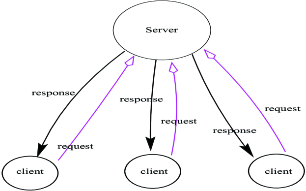
Figure 1: Processing flow between clients and a server

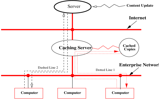
Figure 2: Placement of caching server at an enterprise environment

Web servers and browsers (web clients) are the fundamental architectural building blocks in the World Wide Web. A Web client is a requester of data (content) and a Web server is the provider of data (content). A web server manages and provides data source while Web browsers send requests to a Web server for a specific source data by means of URL (uniform resource locator). Upon receipt of a request initiated by a web client, the web server then processes the request and sends a response back to the web client. Figure 1 illustrates the typical data flow between the clients and the server.

The content resources at servers are autonomous: they are updated independently at various rates without pushing updates to the clients. As a result, each client has to poll the remote resources at a web server periodically in order to detect changes and update its contents. This process is referred to as refresh synchronization. The freshness comes at a cost of resource usage; each request initiated by a client incurs certain communication and computation overhead for processing the request. As a result, it could be very costly in terms of overall bandwidth usage and server load when considering million of individual clients.

Caching is an effective means of reducing the system load of servers and bandwidth usage. The idea behind caching is to store recently retrieved copies of remote source somewhere between the clients and the remote web servers. As a result, the request initiated by a web client can be diverted to the cached copies which are much closer to the Web client than the remote web server in terms of network distance.

The caching architecture in a representative enterprise environment is illustrated in Figure 2 wherein a caching server is placed at the enterprise’s network entrance to external networks, acting as an intermediary between host computers (clients) inside the enterprise network and the internet. Each host machine is connecting to the enterprise’s network backbone, the caching server rests between the enterprise’s network backbone and the Internet. Upon receiving a request originated from a host inside the enterprise’s network, the caching server checks to see whether the corresponding response has already been cached, if the cached file is present, then the caching server returns the client with the cached copy, saving the client from retrieving the same resource (document) repeatedly from the remote server. The flow is represented by the dotted line 1 in Figure 2. If the cached file is absent, the caching server then forwards the request to a server. After the caching server has received the response from the remote server, it returns the response to the client and locally stores the response for subsequent requests. Its is represented by the dashed line 2 in Figure 2. It is clear that the use of caching server in an enterprise environment enables substantial bandwidth saving and dramatically improves user-perceived response time, because the cached copies are located within the vicinity of the clients in terms of network distance. The performance gain appears to be proportional to the number of users [5, 4, 6].

The performance gains of caching carry the cost of content freshness. The cached copies immediately become obsolete as soon as the original copies at the remote server are updated or changed. There is a substantial tradeoff between content freshness and refresh cost: a frequent refresh ensures the freshness of content at high cost of refresh. Conversely, an infrequent refresh inhibits the freshness of content but saves the refresh cost.

Figure 3: Conceptual Flow Diagram of Crawler-based Search Engine

The freshness-cost problem also arises in crawler-based search engine applications. Crawler-based search engines such as google provide a powerful tool for searching web documents, serving as a “yellow book” on the Web. Figure 3 presents a conceptual flow diagram of crawler-based Web search engines. Periodically, a Web search engine polls Web servers independently, and Web clients poll randomly the Web search engine searching for the directories of Web documents. It is clear the refresh scheduling of the web search engine is independent of the Web access by Web clients. In addition, the content at Web servers may change over time and it is impossible to know a priori exactly the arrival time of content update. To maintain the freshness of content, the Web search engine needs to poll web sites and update its database directory in a frequent fashion. Such a process is known as Web crawling. The freshness of content is regarded as one of the important performance metrics for a crawler-based search engine [8]. Web crawling is a prohibitively expensive computation task when considering an astronomical numbers of constantly changing web pages. It is reported that most search engines refresh their entire directory databases once a month [8].

Cho and Garcia-Molina [2, 3] first present a probability model to study the impact of various refresh (synchronization) policies on the content freshness with an emphasis on synchronization-order policy, under different contexts from this paper. Our study in this paper differs from theirs principally in that we consider the problem of refresh scheduling, with the objective of optimally balancing the tradeoff between content freshness and refresh cost.

The remainder of the paper is organized as follows: In Section 2 we consider the problem of refresh scheduling involving one cache element. We study and establish a generic cost model that accounts for both the content freshness and the refresh cost and prove that the mathematical equivalence between the refresh schedulings with the fixed interval and the random interval in terms of the overall refresh cost. Section 3 extends the obtained results into the cases involving more than one cache elements, with an emphasis on the uniform allocation policy. Section 4 concludes the paper.

2 Mathematical Formulation and Main Results

In this section we consider the problem of optimal refresh scheduling involving only one cache element. We begin with an introduction of relevant notions and definitions, followed by a cost analysis of the relationship between the refresh interval and the freshness of content. Finally we identify the optimal refresh frequency that gives the best tradeoff between the content freshness and the refresh cost.

We formally give the notion of the aggregated age function. Our definition is in spirit similar to the one proposed by Cho and Garcia-Molina [3, 2], but differs in the sense that we take the “aggregated effect” of content decay into account. We then introduce the age-related cost function that generalizes the notion of the aggregated age function.

Suppose that the arrival of content update at a server follows the Poisson process with intensity rate of $\lambda$. Let $\{X_{i},i\geq 1\}$ be the interarrival times of the Poisson process. Define $S_{0}=0,~{}S_{n}=\sum\limits_{i=1}^{n}X_{i}$, where $S_{i}$ represents the time of the ith occurrence of content update at the server. Let

$$N(t)=\sup\{n\geq 0:~{}S_{n}\leq t\}.$$ (1)

$N(t)$ is a random variable that represents the number of arrivals of content updates at the server in the time interval $(0,t]$. Two closely related but different notions are given as follows.

Definition 1

Under refresh frequency of $1/T$, the age of the element $e$ with respect to the ith occurrence of content update $S_{i}$ at time $t\in[0,T)$ is

$$Age(e,S_{i},t)=(t-S_{i})I_{\{t>S_{i}\}},$$

where $I_{\{t>S_{i}\}}$ is an indicator function.

$Age(e,S_{i},t)$ is a function representing a measure for the content freshness of the element $e$ with respect to the ith occurrence of content update at the server.

Definition 2

Under refresh frequency of $1/T$, the aggregated age of the element $e$ with respect to the occurrences of content update at time $t\in[0,T)$ is

$$A(e,t)=\sum\limits_{i=1}^{N(t)}(t-S_{i})I_{\{t>S_{i}\}}.$$

$A(e,t)$ is an aggregated age function that reflects the additive effect of multiple content updates taking place within the interval $[0,t)$. Cho and Garcia-Molina [2, 3] propose the age metric as a measure for content freshness by only considering the first occurrence of content update, that is, $Age(e,S_{1},t)$. The major difference between ours and the definition by Cho and Garcia-Molina is that we consider the additive property of content freshness with respect to multiple content updates.

Figure 4 is an illustration of the evolution of the functions of the $A(e,t)$, reflecting that the aggregated age of the element $e$ with respect to the occurrences of content update over time.

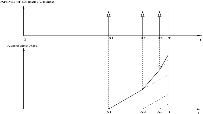
Figure 4: Evolution of Aggregated Age Function of $A(e,t)$

To study the freshness-cost tradeoff, we introduce the age-related cost function denoted by $C_{a}(x)$ which is a nondecreasing and positive function of the age, where the variable $x$ denotes the age of the element of interest and the subscript $a$ the age of content (see Definition 1). The notion of age-related cost is a generalization of the notion of age. As a result, the age function defined in [2] is a special case of the age-related cost function with $C_{a}(x)=x$.

The association of cost with freshness in the problem formulation is partly motivated by its market relevance that many crawler-based search engines such as google, Inktomi and fast [8] introduce paid inclusion programs that trade the freshness of content and visibility for a payment. We further assume that the cost of a refresh synchronization $C_{r}$, where the subscript $r$ indicates the cost associated with refresh. This cost could be a measure of bandwidth usage or latency or a financial payment, depending on the choice of performance metric. The following theorem shows that under mild conditions the optimal refresh interval, $T^{*}$, that minimizes the long-run mean average cost, exists and is unique.

Theorem 1

Suppose that the arrival of update is a Poisson process with intensity rate $\lambda$. Let the refresh interval be $T$, and the cost of a refresh be $C_{r}$. Then the long-run mean average cost of caching under the refresh frequency of $1/T$ is given as

$$C(T)=\frac{C_{r}}{T}+\frac{\lambda\int^{T}_{0}C_{a}(t)dt}{T}.$$ (2)

If the age-related cost function $C_{a}(t)$ satisfies (1) $C_{a}(t)$ is differentiable and $C^{\prime}_{a}(t)>0$; (2) $C_{a}(\infty)=\infty$, then there exists a unique refresh interval, designated $T^{*}$, which minimizes the long-run mean average cost function $C(T)$, and $T^{*}$ is determined by the equation

$$TC_{a}(T)-\int\limits^{T}_{0}C_{a}(t)dt=\frac{C_{r}}{\lambda}.$$

Proof   For a given interval $(0,t]$, the mean average cost over the interval $(0,t]$ can be written as

$$\frac{E(\hbox{the~{}random~{}cost~{}in~{}interval~{}}(0,t])}{t}.$$ (3)

Hence, the long-run mean average cost under the refresh interval $T$ is

$$C(T)=\lim\limits_{t\to\infty}\frac{E(\hbox{the~{}random~{}cost~{}in~{}interval~{}}(0,t])}{t}$$ (4)

if this limit exists. Denote the random cost on the interval $((k-1)T,kT]$ by $\xi_{k}(T),k\geq 1$. Due to the properties of stationary and independent increments of the Poisson process [9], $\xi_{k}(T),k\geq 1$ are iid, the long-run mean average cost can be written as

$$C(T)=\lim\limits_{t\to\infty}\frac{E(\lfloor\frac{t}{T}\rfloor)\xi_{1}(T))}{t}=\frac{E(\xi_{1}(T))}{T},$$ (5)

where the term $\lfloor x\rfloor$ is the floor function that gives the largest integer less than or equal to $x$.

The random cost $\xi_{1}(T)$ on the interval $(0,T]$ consists of a refresh cost and the age-related cost accumulated over the interval $(0,T]$. For the arrival of the nth content update at time $S_{n}\leq T$, the age-related cost, $C_{a}(T-S_{n})$, is a function of the age $T-S_{n}$. The aggregated age-related cost in the interval $(0,T]$ is thus expressed as

$$\sum\limits^{N(T)}_{n=1}\left(C_{a}(T-S_{n})\right)I_{\{N(T)>0\}}.$$

Hence, the random cost $\xi_{1}(T)$ on the interval $(0,T]$ is given as

$$\xi_{1}(T)=C_{r}+\sum\limits^{N(T)}_{n=1}\left(C_{a}(T-S_{n})\right)I_{\{N(T)>0\}}.$$ (6)

Note that

$$\sum\limits^{N(T)}_{n=1}C_{a}(T-S_{n})I_{\{N(T)>0\}}=\sum\limits^{\infty}_{n=1}C_{a}(T-S_{n})I_{\{n\leq N(T)\}}=\sum\limits^{\infty}_{n=1}C_{a}(T-S_{n})I_{\{S_{n}\leq T\}}$$ (7)

and

$$E\left(C_{a}(T-S_{n})I_{\{S_{n}\leq T\}}\right)=\int\limits^{T}_{0}C_{a}(T-t)f_{n}(t)dt,$$ (8)

where $f_{n}(t)$ is the probability density function of $S_{n}$, and follows the gamma distribution as below

$$f_{n}(t)=\frac{\lambda^{n}}{(n-1)!}t^{n-1}e^{-\lambda t},~{}t>0.$$ (9)

Substituting Eq(9) into Eq(8) we obtain

$$E\left(C_{a}(T-S_{n})I_{\{S_{n}\leq T\}}\right)=\int^{T}_{0}C_{a}(T-t)\frac{\lambda^{n}}{(n-1)!}t^{n-1}e^{-\lambda t}dt.$$ (10)

We then have

$$E\left(\sum\limits^{N(T)}_{n=1}C_{a}(T-S_{n})I_{\{N(T)>0\}}\right) = \sum\limits^{\infty}_{n=1}\int^{T}_{0}C_{a}(T-t)\frac{\lambda^{n}}{(n-1)!}t^{n-1}e^{-\lambda t}dt$$ (11)

$$= \int^{T}_{0}C_{a}(T-t)\lambda e^{-\lambda t}\left(\sum\limits^{\infty}_{n=1}\frac{(\lambda t)^{n-1}}{(n-1)!}\right)dt$$

$$= \lambda\int^{T}_{0}C_{a}(T-t)dt=\lambda\int^{T}_{0}C_{a}(t)dt.$$

Therefore, by Eqs(5), (6), and (11), the long-run mean average cost can be expressed as

$$C(T)=\frac{E(\xi_{1}(T))}{T}=\frac{C_{r}}{T}+\frac{\lambda\int^{T}_{0}C_{a}(t)dt}{T}.$$

The derivative of $C(T)$ is then given as

$$C^{\prime}(T)=-\frac{C_{r}}{T^{2}}+\frac{\lambda C_{a}(T)}{T}-\frac{\lambda\int^{T}_{0}C_{a}(t)dt}{T^{2}}.$$

Define a function $\varphi(T)$ as

$$\varphi(T)\equiv T^{2}C^{\prime}(T)=-C_{r}+\lambda TC_{a}(T)-\lambda\int^{T}_{0}C_{a}(t)dt$$ (12)

Observe that $C^{\prime}(T)$ and $\varphi(T)$ have the same sign. It can also be verified that the

$$\varphi^{\prime}(T)=\lambda TC_{a}^{\prime}(T)>0,~{}~{}\forall~{}T>0$$

since $C_{a}^{\prime}(t)>0,\forall t>0$. This shows that the function $\varphi(T)$ strictly increases in $T>0$. Observe that $\varphi(0)=-C_{r}<0$. Moreover, for any fixed $\epsilon>0$, if $T>\epsilon$, then

$$\varphi(T) = -C_{r}+\lambda\int^{T}_{0}\left(C_{a}(T)-C_{a}(t)\right)dt\geq-C_{r}+\lambda\int^{\epsilon}_{0}(C_{a}(T)-C_{a}(t))dt$$ (13)

$$\geq -C_{r}+\lambda(C_{a}(T)-C_{a}(\epsilon))\epsilon$$

Hence $\varphi(\infty)\equiv\lim\limits_{T\to\infty}\varphi(T)=\infty$ since $C_{a}(\infty)=\infty$. Considering the facts that $\varphi(0)<0,~{}\varphi(\infty)=\infty$ and $\varphi(T)$ is strictly increasing in $T>0$, we conclude that there must exist a unique $0<T^{*}<\infty$ such that

$$C^{\prime}(T)=\left\{\begin{array}[]{ll}<0,&\hbox{ if }0<T<T^{*}\\ =0,&\hbox{ if }T=T^{*}\\ >0,&\hbox{ if }T>T^{*}.\end{array}\right.$$

Therefore, $T^{*}$ minimizes $C(T)$, or

$$T^{*}=\arg\left(\min\limits_{T>0}C(T)\right).$$

 

Corollary 1

Suppose that the age-related cost function $C_{a}(t)=Ct$, where $C>0$ is the proportionality constant. Then the long-run mean average cost function $C(T)$ is given as

$$C(T)=\frac{C_{r}}{T}+\frac{C\lambda T}{2}$$ (14)

and is minimized at

$$T^{*}=\sqrt{\frac{2C_{r}}{\lambda C}}.$$ (15)

Also, $C(T^{*})=\sqrt{2\lambda CC_{r}}$.

Proof   Obviously $C_{a}(t)=Ct$ satisfies the condition in Theorem 1. Thus, $T^{*}\equiv\arg(\min\limits_{T>0}C(T))$ exists and is uniquely determined by the equation $C^{\prime}(T)=0$ where

$$C^{\prime}(T)=-\frac{C_{r}}{T^{2}}+\frac{\lambda C}{2}$$

and the unique solution to $C^{\prime}(T)=0$ is given by

$$T^{*}=\sqrt{\frac{2C_{r}}{\lambda C}}$$

.  

From Corollary 1, it is shown that the optimal refresh interval decreases with increasing rate of the content update when the age function is linear. This result, however, is also true in general as shown in the following theorem.

Theorem 2

Under the same conditions of Theorem 1, the optimal refresh interval $T^{*}$ strictly decreases in $\lambda>0$.

Proof   Clearly $T^{*}$ is a function of $\lambda$. For the sake of simplicity, we will not express this dependence explicitly. For the same reason we will suppress the symbol $*$ and just use $T$ to denote the optimal refresh interval in the following derivation. From Theorem 1, the optimal refresh interval satisfies $\varphi(T)=0$, or

$$-C_{r}+\lambda TC_{a}(T)-\lambda\int^{T}_{0}C_{a}(t)dt=0.$$ (16)

Taking derivative with respect to $\lambda$ in Eq(16), we obtain

$$TC_{a}(T)+\lambda TC_{a}^{\prime}(T)\frac{dT}{d\lambda}-\int^{T}_{0}C_{a}(t)dt=0.$$ (17)

From Eq(17) it follows that

$$\lambda TC_{a}^{\prime}(T)\frac{dT}{d\lambda} = \int^{T}_{0}C_{a}(t)dt-TC_{a}(T)$$ (18)

$$= \int^{T}_{0}\left(C_{a}(t)-C_{a}(T)\right)dt<0.$$

Eq(18) immediately implies

$$\frac{dT^{*}(\lambda)}{d\lambda}<0$$

since $C_{a}^{\prime}(T)>0$. This proves that $T^{*}=T^{*}(\lambda)$ is a strictly decreasing function of $\lambda$.  

Theorem 3

Under the same conditions of Theorem 1, the fixed optimal refresh policy $T^{*}$ strictly increases in $C_{r}>0$.

The proof is simple and straightforward, therefore is omitted.

Remark 1: Theorems 2, 3 demonstrate that the impact of the arrival rate of content update as well as the refresh overhead $C_{r}$ on the optimal refresh frequency. A high frequency of content update and cheap refresh cost exact a high frequency of refresh in order to maintain a certain level of content freshness. Conversely, an infrequent content update and expensive refresh cost require refresh be performed at low frequency in order to save bandwidth usage and mitigate server load. This analytical results obtained above not only agree well with our intuition, but also provide us with a quantitative connection between optimal refresh interval and arrival rate of update.

Theorem 4

Suppose that two age-related cost functions $C_{a1}(t)$ and $C_{a2}(t)$ satisfy the conditions in Theorem 1. Let $T{}^{*}_{1}$ and $T{}^{*}_{2}$ be the optimal refresh intervals associated with $C_{a1}(t)$ and $C_{a2}(t)$, respectively. For given $C_{r}$ and $\lambda$, if $0\leq\Delta(t)\equiv C_{a2}(t)-C_{a1}(t)$ is nondecreasing in $t\geq 0$, then $T{}^{*}_{1}\geq T{}^{*}_{2}$.

Proof   According to the proof of Theorem 1, it is shown that

$$\varphi(T)\equiv-C_{r}+\lambda TC_{a1}(T)-\lambda\int^{T}_{0}C_{a1}(t)dt$$ (19)

strictly increases in $T$, and

$$\varphi(T{}^{*}_{1})=-C_{r}+\lambda T{}^{*}_{1}C_{a1}(T{}^{*}_{1})-\lambda\int^{T_{1}^{*}}_{0}C_{a1}(t)dt=0.$$ (20)

Suppose that contrary to the claimed result, i.e., $T{}^{*}_{1}<T{}^{*}_{2}$. From the monotonicity of $\varphi(T)$ in Eq(12) and $\varphi(T{}^{*}_{1})=0$, we have $\varphi(T{}^{*}_{2})>0$. That is

$$-C_{r}+\lambda T{}^{*}_{2}C_{a1}(T{}^{*}_{2})-\lambda\int^{T{}^{*}_{2}}_{0}C_{a1}(t)dt>0.$$ (21)

Note that

$$-C_{r}+\lambda T{}^{*}_{2}C_{a2}(T{}^{*}_{2})-\lambda\int^{T{}^{*}_{2}}_{0}C_{a2}(t)dt$$ (22)

$$= -C_{r}+\lambda T^{*}_{2}C_{a1}(T^{*}_{2})+\lambda T^{*}_{2}\Delta(T^{*}_{2})-\lambda\int^{T^{*}_{2}}_{0}C_{a1}(t)dt+\lambda\int^{T^{*}_{2}}_{0}\Delta(t)dt$$

$$= \left\{-C_{r}+\lambda T^{*}_{2}C_{a1}(T^{*}_{2})-\lambda\int^{T{}^{*}_{2}}_{0}C_{a1}(t)dt\right\}+\lambda\left\{T^{*}_{2}\Delta(T^{*}_{2})-\int^{T^{*}_{2}}_{0}\Delta(t)dt\right\}$$

$$= \varphi(T^{*}_{2})+\lambda\int^{T^{*}_{2}}_{0}\left(\Delta(T^{*}_{2})-\Delta(t)\right)dt$$

$$\geq \varphi(T^{*}_{2})>0,$$

where Eq(22) comes directly from the assumption that $\Delta(t)$ is nondecreasing in $t\geq 0$. However, as the optimal refresh policy associated with $C_{a2}(t)$, it must be true that

$$-C_{r}+\lambda T^{*}_{2}C_{a2}(T^{*}_{2})-\lambda\int^{T^{*}_{2}}_{0}C_{a2}(t)dt=0$$

which contradicts with the inequality (22). Therefore, we must have $T^{*}_{1}\geq T^{*}_{2}$.  

In the previous discussion we assume that refresh interval has a fixed length of $T$. This assumption is somewhat unrealistic in practice. In the following, we study the impact of random refresh scheduling on the long-run mean average cost.

Let $\{Y_{i},i\geq 1\}$ be a sequence of iid random variables defined on $(0,\infty)$ following certain distribution $H$. The sequence $\{Y_{i},i\geq 1\}$ representing the interarrival times under a random refresh scheduling is assumed to be independent of the Poisson arrival of content update at a server. It is obvious that a fixed refresh policy is only a special case of a random refresh policy.

Let ${\cal H}$ be the family of all distribution functions on $(0,\infty)$ with finite first moment. Namely,

$${\cal H}=\left\{H\colon~{}H\hbox{~{}is~{}a~{}CDF ~{}on~{}$(0,\infty)$~{}and~{}}\int^{\infty}_{0}\bar{H}(t)dt<\infty\right\}$$

where $\bar{H}(t)\equiv 1-H(t),~{}\forall t\geq 0$.

Theorem 5

Let $C_{H}(\cdot)$ denote the long-run mean average cost under a random refresh interval $Y$ characterized by certain distribution function $H\in{\cal H}$, and $C(T)$ denote the long-run mean average cost under fixed refresh scheduling with interval $T$, then

$$\min\limits_{H\in{\cal{H}}}C_{H}=\min\limits_{T>0}C(T).$$

Proof   Since the sequence $\{Y_{i},i\geq 1\}$ of interarrival refresh times is independent of the Poisson arrival of content update, it is easy to see that the random costs over the intervals $(0,Y_{1}],(Y_{1},Y_{1}+Y_{2}],\ldots$ are iid. Using the same line as the proof of Theorem 1, the long-run mean average cost is expressed as

$$C_{H}=\frac{E(\hbox{random~{}age-related~{}cost~{}over~{}}(0,Y])}{E(Y)},$$

where $Y$ has distribution $H$. Let $\xi(Y)$ be the random cost in the cycle $(0,Y]$, we have

$$E(\xi(Y)) = E\{E[\xi(Y)|Y]\}$$ (23)

$$= \int^{\infty}_{0}E(C_{r}+\sum\limits^{N(y)}_{n=1}C_{a}(y-S_{n})I_{\{N(y)>0\}})dH(y),$$

where $S_{n}=\sum\limits^{n}_{i=1}X_{i}$ denotes the time of the nth arrival of content update at the server. Due to the independence of $\{X_{i},i\geq 1\}$ and $\{Y_{i},i\geq 1\}$, from Eq(23) we further obtain

$$E(\xi(Y)) = \int^{\infty}_{0}(C_{r}+\int^{y}_{0}\lambda C_{a}(t)dt)dH(y)$$

$$= C_{r}+\int^{\infty}_{0}\left(\int^{y}_{0}\lambda C_{a}(t)dt\right)dH(y).$$

Therefore, the long-run expected average cost is expressed as

$$C_{H}=\frac{C_{r}}{E(Y)}+\frac{\int^{\infty}_{0}\left(\int^{y}_{0}\lambda C_{a}(t)dt\right)dH(y)}{E(Y)}.$$ (24)

It is straightforward that

$$\min\limits_{H\in\cal{H}}C_{H}\leq\min\limits_{T>0}C(T)$$ (25)

since a fixed refresh scheduling with the interval $T>0$ is a degenerate random refresh scheduling when $P(Y=T)=1$.

Now for any given random refresh scheduling $Y$ with distribution $H\in{\cal{H}}$. Eq(24) can be reexpressed as

$$C_{H} = \frac{C_{r}}{E(Y)}+\frac{\int^{\infty}_{0}\left(\int^{\infty}_{t}\lambda C_{a}(t)dH(y)\right)dt}{E(Y)}$$ (26)

$$= \frac{C_{r}}{E(Y)}+\frac{\lambda\int^{\infty}_{0}C_{a}(t)\bar{H}(t)dt}{E(Y)}.$$

If we choose $T=E(Y)\equiv\mu$, meaning that the fixed refresh interval $T$ equals to the mean value of the random refresh interval $Y$, then according to Eq(2), we have

$$C(T)=\frac{C_{r}}{\mu}+\frac{\lambda\int^{\mu}_{0}C_{a}(t)dt}{\mu}.$$ (27)

Subtracting Eq(27) from Eq(26), we obtain

$$C_{H}-C(T) = \frac{\lambda}{\mu}\left\{\int^{\infty}_{0}C_{a}(t)\bar{H}(t)dt-\int^{\mu}_{0}C_{a}(t)dt\right\}$$ (28)

$$= \frac{\lambda}{\mu}\left\{\int^{\mu}_{0}C_{a}(t)\bar{H}(t)dt+\int^{\infty}_{\mu}C_{a}(t)\bar{H}(t)dt-\int^{\mu}_{0}C_{a}(t)dt\right\}$$

$$= \frac{\lambda}{\mu}\left\{\int^{\infty}_{\mu}C_{a}(t)\bar{H}(t)dt-\int^{\mu}_{0}C_{a}(t)H(t)dt\right\}$$

$$\geq \frac{\lambda}{\mu}\left\{C_{a}(\mu)\int^{\infty}_{\mu}\bar{H}(t)dt-C_{a}(\mu)\int^{\mu}_{0}H(t)dt\right\}$$

$$= \frac{\lambda C_{a}(\mu)}{\mu}\left\{\int^{\infty}_{\mu}\bar{H}(t)dt-\int^{\mu}_{0}(1-\bar{H}(t))dt\right\}$$

$$= \frac{\lambda C_{a}(\mu)}{\mu}\left\{\int^{\infty}_{0}\bar{H}(t)dt-\mu\right\}=0$$

thus we have

$$C_{H}\geq C(T)$$ (29)

Combining Eq(25) and Eq(29), we obtain

$$\min\limits_{H\in{\cal{H}}}C_{H}=\min\limits_{T>0}C(T)$$

 

Such a mathematical equivalence between fixed refresh and random refresh schedulings offers a theoretical justification for the flexibility that is needed in real application environments. Refresh scheduling with random variable $Y$ over a finite interval $(a,b)$ is more flexible than fixed refresh scheduling. Let $T>0$ be a given fixed refresh interval and $Y$ be a positive random interval following a distribution on interval $(a,b)$ with mean $E(Y)=T$. From Eq(29) it can be seen that $C_{H}\geq C(T)$ and the equality holds if and only if $Y$ is a degenerate random variable when $P(Y=T)=1$. Thus, for any given $T>0,\delta>0$ satisfying $T-\delta>0$, if we denote ${\cal H}^{*}=\{\mbox{H : H is a CDF on }(T-\delta,T+\delta)\mbox{ and }\int_{T-\delta}^{T+\delta}tdH(t)=T\}$, then we have $C_{H}>C(T)$ for any non-degenerate $H\in{\cal H}^{*}$. In particular, if $U(\delta)$ is the uniform distribution on $(T-\delta,T+\delta)$, then it is true that $C_{U(\delta)}>C(T)$. It is also easy to show that $\lim_{\delta\rightarrow 0}C_{U(\delta)}=C(T)$.

3 Synchronizing Multiple Content Elements

In the section we will extend this approach to the case that involves more than one elements with different content update rates.

Consider a server containing content elements $S=\{e_{1},\cdots,e_{M}\}$. Each element $e_{i}$ is being updated according to a Poisson process with intensity $\lambda_{i}$ ($1\leq i\leq M$). It is theoretically appealing to synchronize each content element $e_{i}$ using refresh interval $T_{i}$, which is referred to as non-uniform allocation policy [2, 3]. However, uniform allocation policy [2, 3], i.e., synchronizing all content elements by using the same refresh interval $T$, is practically preferable by amortized cost analysis. The underlying reason is that each refresh requires a connection establishment along with bandwidth usage and processing overhead. A connection overhead (latency) denoted as $C_{conn}$ is considered as the dominating factor in determining refresh cost $C_{r}$. The advantage of the uniform allocation policy over the non-uniform allocation policy is its ability to share its connection cost over the number of the content elements. As a result, the amortized connection for the uniform allocation policy is calculated as $C_{conn}/M$, which is much cheaper than that of the non-uniform allocation policy, $C_{conn}$.

Let $\lambda_{i}$ be the intensity rate of Poisson process describing the content update of the cache element $e_{i}$, $1\leq i\leq M$. From Theorem 1, the long-run mean average cost of caching over the entire $S$ is

$$C(T)=\sum_{i=1}^{M}\bigl{[}\frac{C_{r}(\lambda_{i})}{T}+\frac{\lambda_{i}\int^{T}_{0}C_{a}(t;\lambda_{i})dt}{T}\bigr{]},$$

where $C_{r}(\lambda_{i})$ is the cost associated with a refresh of element $e_{i}$, and $C_{a}(t;\lambda_{i})$ is the age-related cost function associated with element $e_{i}$, if the uniform allocation policy $T$ is applied. Then $C(T)$ can be rewritten as

$$C(T)=M[\frac{\bar{C}_{r}}{T}+\frac{\int^{T}_{0}\bar{C}_{a}(t)dt}{T}],$$ (30)

where

$$\bar{C}_{r}=\frac{\sum_{i=1}^{M}C_{r}(\lambda_{i})}{M}$$ (31)

and

$$\bar{C}_{a}(t)=\frac{\sum_{i=1}^{M}\lambda_{i}C_{a}(t;\lambda_{i})}{M}.$$ (32)

If the size of the set of cache elements, $M$, is sufficiently large, then it is convenient to describe all $\lambda_{i}$ by a probability density function $g(\lambda)$ on $(0,\infty)$. With this assumption, the long-run mean average cost of caching the entire set of elements $S$ is given as

$$C(T)=M[\frac{\bar{C}_{r}}{T}+\frac{\int^{T}_{0}\bar{C}_{a}(t)dt}{T}],$$ (33)

where

$$\bar{C}_{r}=\int_{0}^{\infty}C_{r}(\lambda)g(\lambda)\,d\lambda$$

and

$$\bar{C}_{a}(t)=\int_{0}^{\infty}\lambda C_{a}(t;\lambda)g(\lambda)\,d\lambda.$$

Combining Eq(30) and Eq(33), we see that minimizing $C(T)$ is equivalent to minimizing

$$\frac{\bar{C}_{r}}{T}+\frac{\int^{T}_{0}\bar{C}_{a}(t)dt}{T}.$$ (34)

Since the form of Eq(34) is the same as Eq(2), we immediately obtain the following result.

Theorem 6

Suppose that the arrival of update of each content $e$ is a Poisson process with intensity rate $\lambda$, $C_{r}(\lambda)$ is the cost associated with a refresh, and the refresh interval is $T$. Then the long-run mean average cost of caching $S$ is given as

$$C(T)=M\bigl{[}\frac{\bar{C}_{r}}{T}+\frac{\int^{T}_{0}\bar{C}_{a}(t)dt}{T}\bigr{]},$$

where

$$\bar{C}_{r}=\int_{0}^{\infty}C_{r}(\lambda)\,dG(\lambda),$$

$$\bar{C}_{a}(t)=\int_{0}^{\infty}\lambda C_{a}(t;\lambda)\,dG(\lambda),$$

and $G(\lambda)$ is a distribution function on $(0,\infty)$ satisfying $\int_{0}^{\infty}\lambda C_{a}(t;\lambda)\,dG(\lambda)<\infty$ for any $t>0$. The problem of minimizing $C(T)$ is equivalent to minimizing $\bar{C}(T)$ given as

$$\bar{C}(T)=\frac{\bar{C}_{r}}{T}+\frac{\int^{T}_{0}\bar{C}_{a}(t)dt}{T}.$$ (35)

If the age-related cost function $\bar{C}_{a}(t)$ satisfies (a) $\bar{C}^{\prime}_{a}(t)>0$; (b) $\bar{C}_{a}(\infty)=\infty$, then there exists unique refresh interval, designated $T^{*}$, which minimizes $C(T)$ and $\bar{C}(T)$. Moreover, $T^{*}$ is determined by the equation

$$T\bar{C}_{a}(T)-\int\limits^{T}_{0}\bar{C}_{a}(t)dt=\bar{C}_{r}.$$

4 Conclusion

There is a fundamental tradeoff between the freshness of content and the overhead of refresh synchronization. An excessive refresh puts a strain on computation resource of network bandwidth and servers, while a deficient refresh sacrifices the required freshness of content. This paper is focused on studying the effect of refresh scheduling on the freshness-cost tradeoff. We formulate the refresh scheduling problem with a generic cost model to capture the relationship between the arrival rate of content update, the freshness of content and the cost of refresh synchronization, and then use this cost model to determine an optimal refresh interval that minimizes the overall cost involved.

Theoretical results obtained in this paper suggest that the optimal refresh frequency should be a function of the arrival rate of content update and the refresh cost, implying that refresh frequency is determined by the arrival rate of content update in order to maintain a certain level of content freshness. Such a viewpoint has been implicitly reflected in the fact that many crawler-based Web search engines like google, Inktomi and fast started developing an automated tool to identify the content change rate at some Web sites, and adapt refresh rate to the actual changing rate of content sources [8]. This paper gives a quantitative analysis of the freshness-cost tradeoff and offers a theoretical guidance in determining the best tradeoff between the freshness of content and the cost of refresh synchronization.

5 Acknowledgement

The authors would like to thank anonymous referees for their insightful comments on a preliminary version of this paper.

References

- [1] Cnn delivers unprecedented online service. In http://www.volera.com/corporate/pressroom/casestudies/cnn.html.
- [2] Junghoo Cho and Hector Garcia-Molina. The evolution of the web and implications for an incremental crawler. In Proceedings of the Twenty-sixth International Conference on Very Large Databases, 2000.
- [3] Junghoo Cho and Hector Garcia-Molina. Synchronizing a database to improve freshness. In Proceedings of the 2000 ACM International Conference on Management of Data, June 2000.
- [4] Edith Cohen and Haim Kaplan. Age penalty and its effects on cache performance. In The 3rd USENIX Symposium On Internet Technologies and Systems, March 2001.
- [5] Edith Cohen and Haim Kaplan. Refreshment policies for web content caches. In Proceedings of Proceedings of the IEEE INFOCOM’01 Conference, 2001.
- [6] Bradley M. Duska, David Marwood, and Michael J. Feeley. The measured access characteristics of world-wide-web client proxy caches. In Proceedings of the USENIX Symposium on Internet Technologies and Systems, December 1997.
- [7] Kang-Won Lee, Khalil Amiri, S. Sahu, and Chitra Venkatramani. On the sensitivity of cooperative caching performance to workload and network characteristics. In Proceedings of the ACM Conference on Measurement and Modeling of Computer SystemS (SIGMETRICS), 2002.
- [8] Greg Notess. Freshness issue and complexities with web search engines. OnLine, 25(6), November 2001.
- [9] Sheldon M. Ross. Stochastic Processes. John Wiley & Sons, Inc., New York, 1996.
- [10] Duane Wessels. Web Caching. O’Reilly & Associates, Inc, USA, 2001.