Filter diagonalization of shell-model calculations

Abstract

We present a method of filter diagonalization for shell-model calculations. This method is based on the Sakurai and Sugiura (SS) method, but extended with help of the shifted complex orthogonal conjugate gradient (COCG) method. A salient feature of this method is that it can calculate eigenvalues and eigenstates in a given energy interval. We show that this method can be an alternative to the Lanczos method for calculating ground and excited states, as well as spectral strength functions. With an application to the $M$-scheme shell-model calculations we demonstrate that several inherent problems in the widely-used Lanczos method can be removed or reduced.

I Introduction

To perform numerical investigations of quantum many-body systems, many approaches have been proposed, e.g., exact diagonalization, the quantum Monte Carlo method, the density matrix renormalization group method, and so on. To compare with other approaches, the exact diagonalization method has a broader range of applications, and can calculate energies and wave functions without any approximation. While a required dimensionality for the Hilbert space is huge, the matrix dimension that can be handled in the exact diagonalization approach has recently increased dramatically, owing to the development of computers. Hence, the diagonalization method has become a basic tool in numerical studies, and has played an important role in various fields of sciences. As for instance, in nuclear structure physics, the exact diagonalization method is of primary importance for shell-model calculations.

For an exact diagonalization in large-scale shell-model calculations, the Lanczos method Lanczos has so far been the only feasible method for practical use. This method has been widely employed to obtain not only ground states but also low-lying excited states. Nevertheless, there still exist three long-standing problems: (1) In calculating highly excited states, convergence is much slower than that for the ground and low-lying states. The number of the Lanczos iteration process tends to grow rapidly as the energy goes higher. (2) The Lanczos method needs to do reorthogonalization of all obtained Lanczos vectors, which demands substantial numerical effort. This problem is rather technical but crucial in practice because the reorthogonalization procedure sets a practical limitation in solving highly excited states. (3) In large-scale shell-model calculations with the $M$-scheme, the total angular momentum $J$ and the total isospin $T$ are not necessarily conserved for each basis, although the total magnetic quantum number $J_{z}=M$ is conserved by definition. Then conservation of angular momentum and isospin may be violated in some cases. In the Lanczos method, conservations of $J$ and $T$ can be realized by choosing an initial wave function with good quantum numbers $J$ and $T$. However, this procedure is not so stable against round-off errors. Therefore, the conservation of these quantum numbers is an important issue particularly in the $M$-scheme shell-model calculations.

Up to now, several shell-model codes antoine ; horoi ; mshell have been developed for state-of-the-art large-scale calculations. However, there has been no attempt to solve the long-standing and basic problems in the Lanczos method mentioned above.

Recently Sakurai and Sugiura (SS) SS1 ; SS2 have proposed a new diagonalization method for a generalized eigenvalue problem: $Ax=\lambda Bx$, where $A$ and $B$ are arbitrary matrices (i.e., not necessarily symmetric matrices). Their method is applicable even to complex matrices. In this method, Cauchy’s integral formula is used in order to obtain eigenvalues (and associated eigenvectors) inside of the region enclosed by a given integration contour, which can be considered to be a kind of a filter. Therefore we call this new method gfilter diagonalization h hereafter.

In the SS method, a diagonalization problem turns into a problem of solving a large number of linear equations, which also demands a heavy computation for large-scale shell-model calculations. To overcome this difficulty, we use the shifted complex orthogonal conjugate gradient (COCG) method shiftedCOCG . The shifted COCG method corresponds to a combination of “shift” algorithms shifts and the COCG method COCG , which is designed to solve a particular family of linear equations. An advantage of the shifted COCG method is that a problem of diagonalization can be reduced to just one linear equations. With the help of the shifted COCG method, the SS method is greatly reinforced and becomes more feasible. The first study on the SS method with the shift algorithms was presented in Ref.Ogasawara . Very recently, an application and an extension of the SS method with the shift algorithms have been reported for all-to-all propagators in the lattice quantum chromodynamics (QCD) QCD .

In this paper, we apply the filter diagonalization based on the SS method combined with the shifted COCG to quantum many-body systems, and demonstrate that the filter diagonalization is indeed an alternative to the Lanczos method in evaluating energy eigenvalues, eigenstates and spectral strength functions. Moreover, the aforementioned problems of the Lanczos method in the $M$-scheme shell-model calculations are shown to be removed or reduced.

This paper is organized as follows: In Sec. II, we show the filter diagonalization based on the SS method and the shifted COCG method, and present how to evaluate the spectral strength function. In Sec. III, we present several examples of numerical calculations and discuss characteristic properties of the method. In Sec. IV, we give a conclusion. In Appendices, we summarize useful relations concerning the Hankel matrix and an algorithm of the shifted COCG method. For readers who have interest in this diagonalization, this paper is written in a self-contained manner.

II Filter diagonalization of shell-model calculations

II.1 SS method

In this section, we summarize the SS method in the shell-model calculations. In order to reduce a large-scale eigenvalue problem to a small scale one, we first consider moments $\mu_{p}(p=0,1,2,\cdots)$ defined by Cauchy’s integral as,

$$\mu_{p}=\frac{1}{2\pi i}\int_{\Gamma}\langle\psi|\frac{(z-\epsilon)^{p}}{z-H}|\phi\rangle dz,$$ (1)

where $|\psi\rangle$ and $|\phi\rangle$ are arbitrary wave functions, and $H$ is a shell-model Hamiltonian, satisfying the eigenvalue equation $H|\varphi_{i}\rangle=e_{i}|\varphi_{i}\rangle$. $\epsilon$ denotes the energy in the vicinity of an energy region of interest (target region). $\Gamma$ means an integration contour to enclose energy eigenvalues in the target region, as depicted in Fig. 1. The integration is carried out on the complex $z$ plane, so that energy eigenvalues on the real axis are energy poles if they are inside the integration contour $\Gamma$. As a result, these eigenvalues contribute to the integral, and they are central quantities in the SS method SS1 .

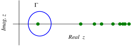
Figure 1: (Color online) An illustration of integration contour $\Gamma$ (an open circle) and energy poles (filled circles) on the complex $z$-plane. In this illustration, $\Gamma$ encloses one of the energy poles on the real-$z$ axis.

To clarify the physical meaning of these moments, we expand $|\psi\rangle$ and $|\phi\rangle$ in terms of the ortho-normalized energy eigen functions $|\varphi\rangle^{\prime}s$ of the Hamiltonian $H$, that is, $|\psi\rangle=\displaystyle\sum c_{i}|\varphi_{i}\rangle$ and $|\phi\rangle=\displaystyle\sum d_{i}|\varphi_{i}\rangle$, where $c$’s and $d$’s are coefficients with $\displaystyle\sum|c{}_{k}|^{2}=1$ and $\displaystyle\sum|d_{k}|^{2}=1$.

Due to the theorem of residue, Cauchy’s integral is formally carried out and the moments are rewritten as

$$\mu_{p}=\sum_{k\in\Gamma}(e_{k}-\varepsilon)^{p}c_{k}d_{k}.$$ (2)

The summation over $k$ is taken if energy eigenvalues are inside the $\Gamma$. The moment $\mu_{p}$ vanishes when none of the energy poles is enclosed by $\Gamma$, or when amplitude is zero for the eigenstates corresponding to the poles (i.e., $c_{k}d_{k}=0$).

To extract the energy eigenvalues $e_{k}(k\in\Gamma)$ from these moments, we follow the SS method SS1 . Namely, we solve the generalized eigenvalue problem formulated as

$$Mx=\lambda Nx,$$ (3)

where $M$ and $N$ are the $n\times n$ Hankel matrices defined by

$$M=\left(\begin{array}[]{cccc}\mu_{1},&\mu_{2},&\cdots&\mu_{n}\\ \mu_{2},&\mu_{3},&\cdots&\mu_{n+1}\\ \vdots&&\ddots&\vdots\\ \mu_{n},&\mu_{n+1},&\cdots&\mu_{2n-1}\end{array}\right),$$ (4)

and

$$N=\left(\begin{array}[]{cccc}\mu_{0},&\mu_{1},&\cdots&\mu_{n-1}\\ \mu_{1},&\mu_{2},&\cdots&\mu_{n}\\ \vdots&&\ddots&\vdots\\ \mu_{n-1},&\mu_{n},&\cdots&\mu_{2n-2}\end{array}\right).$$ (5)

It is then possible to demonstrate that the eigenvalues $\lambda_{k}$ in the generalized eigenvalue equation correspond to $e_{k}-\varepsilon.$ Its proof needs a property of the Hankel matrices that they can be always factorized with the Vandermonde matrix SS1 , as shown in Appendix A. Note that this method to extract eigenvalues from moments was used in Ref. whitehead .

The dimension $n$ introduced in the generalized eigenvalue equation corresponds to the number of eigenvalues inside the integration contour, but it is not known a priori. The optimum $n$ can be obtained by monitoring a convergence pattern of the energy eigenvalues as a function of $n$. This is because the energy eigenvalues should be unchanged when the $n$ exceeds the number of eigenvalues inside the integration contour.

The amplitude $c_{k}d_{k}$ of $(e_{k}-\varepsilon)^{p}$ in Eq. (2) can be obtained by the diagonal matrix given as

$$D=V^{-1}N(V^{T})^{-1},$$ (6)

where $V$ is a Vandermonde matrix defined by $V_{ij}=(e_{j}-\varepsilon)^{i-1}$, i.e.,

$$V^{T}=\left(\begin{array}[]{cccc}1,&e_{1}-\epsilon,&\cdots&(e_{1}-\epsilon)^{n-1}\\ 1,&e_{2}-\epsilon,&\cdots&(e_{2}-\epsilon)^{n-1}\\ \vdots&&\ddots&\vdots\\ 1,&e_{n}-\epsilon,&\cdots&\left(e_{n}-\epsilon\right)^{n-1}\end{array}\right)$$ (7)

because of Eq. (40) in Appendix A. It should be noted here that inverse operations of the Vandermonde matrix are not numerically stable. It is thus better to use the eigenvectors in the generalized eigenvalue equation in practical calculations, because $(V^{T})^{-1}$ is equivalent to the eigenvectors of Eq. (3).

To study electromagnetic transition properties, wave functions should be described in the framework of the SS method. For this purpose, we define vectors $|s_{p}\rangle$ as

$$|s_{p}\displaystyle\rangle=\frac{1}{2\pi i}\int_{\Gamma}\frac{(z-\epsilon)^{p}}{z-H}|\phi\rangle dz.$$ (8)

In the same way as Eq. (2), this can be also formally rewritten as

$$|s_{p}\displaystyle\rangle=\sum_{k\in\Gamma}d_{k}|\phi_{k}\rangle(V^{T})_{kp}.$$ (9)

Therefore, wave functions $|\phi_{k}\rangle$ are explicitly obtained as,

$$|\displaystyle\phi_{k}\rangle\propto\sum_{p}|s_{p}\rangle(V^{T})_{pk}^{-1}.$$ (10)

Its general proof is shown in Ref. SS1 .

An error analysis was presented for the Hankel and Vandermonde matrices in the context of the SS method, in Refs. Erroranalysis .

II.2 Numerical integration, scaling, and shifted COCG method

Next, we explain how to integrate the moments $\mu_{p}$. An integration contour $\Gamma$ is chosen to be a circle given as,

$$z=\varepsilon+re^{i\theta}\ \ (\varepsilon,r:{\rm real},\ \ \theta=[0,2\pi]).$$ (11)

The target eigen energies are then located between $\varepsilon-r$ and $\varepsilon+r$. Cauchy’s integral is now evaluated numerically by the trapezoidal rule with respect to angle $\theta$ as

$$\mu_{p}\sim\frac{1}{N_{0}}\sum_{k=0}^{N_{0}-1}\langle\psi|\frac{(z_{k}-\epsilon)^{p+1}}{z_{k}-H}|\phi\rangle,$$ (12)

where $z_{k}=\varepsilon+re^{i\frac{2\pi}{N_{0}}(k+\frac{1}{2})}$. Here, we take integral points in a symmetric manner about the real axis because we take an advantage of the property $f(\overline{z})=\overline{f(z)}$ for a complex number $z$.

The integration contour with a larger $r$ can include more energy poles. However, as the $\mu_{p}$ has the $r^{p}$ dependence, the moments become larger as a function of $p$, which causes a numerical instability in Eq. (3). To remove it, we scale Eq. (1) by mapping the circle with radius $r$ into a unit circle SS2 as

$$z^{\prime}=z/r=\varepsilon/r+e^{i\theta}.$$ (13)

Under this mapping, the moments $\mu_{p}^{\prime}$ become

$$\mu_{p}^{\prime}=\sum_{k\in\Gamma}(\frac{e_{k}-\varepsilon}{r})^{p}c_{k}d_{k},$$ (14)

where $\mu_{p}^{\prime}=\mu_{p}/r^{p}$. Then, the $r^{p}$ dependence is removed in

$$\mu_{p}^{\prime}\sim\frac{1}{N_{0}}\sum_{k=0}^{N_{0}-1}\langle\psi|\frac{(z_{k}^{\prime}-\epsilon^{\prime})^{p+1}}{z_{k}^{\prime}-H^{\prime}}|\phi\rangle,$$ (15)

where $z_{k}^{\prime}=z_{k}/r$, $H^{\prime}=H/r$ and $\epsilon^{\prime}=\epsilon/r$.

For each angle $\theta$, we need to evaluate a matrix element $\displaystyle\langle\psi|\frac{1}{z-H}|\phi\rangle$, which involves an inverse operator. To avoid handling inverse operators, we define $|\chi\rangle$ as

$$|\phi\rangle=(z-H)|\chi\rangle,$$ (16)

and calculate $|\chi\rangle$ first, then obtain $\displaystyle\langle\psi|\frac{1}{z-H}|\phi\rangle=\langle\psi|\chi\rangle.$

To obtain $|\chi\rangle$, we solve linear equations; $Ax=b$, where $A_{m,n}=\langle m|z-H|n\rangle$, $b_{m}=\langle m|\phi\rangle$ and $x_{m}=\langle m|\chi\rangle$. A vector $|m\rangle$ means an $M$-scheme basis. This equation is solved by the COCG method COCG for complex, symmetric, but non-hermitian matrices, because complex number $z$ appears in the diagonal matrix elements. As $|\chi\rangle$ depends on $z$, the above linear equations should be solved for each $z$. As the number of integral points $N_{0}$ increases, this numerical calculation becomes more time-consuming. However, by using an invariance property of the Krylov subspace, we can drastically reduce the amount of computation. Once we can solve $|\phi\rangle=(z_{0}-H)|\chi_{0}\rangle$ at a certain $z_{0}$ by the COCG method and store residual vectors, we can compute $|\phi\rangle=(z-H)|\chi\rangle$ for $z\sim z_{0}$ from the stored residual vectors. This method is called the shifted COCG method shiftedCOCG ; CGMEMO . Details are shown in Appendix B. We will present how to reduce computation by this method in Sec. III. B.

II.3 Spectral strength function

To investigate a dynamic property of a system concerning an operator $O$, it is useful to evaluate a spectral strength function $I\left(\omega\right)$ defined as,

$$I\displaystyle\left(\omega\right)=\sum_{n}|\langle\psi_{n}^{(B)}|O|\psi_{0}^{(A)}\rangle|^{2}\delta\left(\omega-(E_{n}^{(B)}-E_{0}^{(A)})\right),$$ (17)

where $E_{n}^{(B)}$ and $E_{0}^{(A)}$ are energies of the $n$-th state and the 0-th state, respectively, and $|\psi_{n}^{(B)}\rangle$ and $|\psi_{0}^{(A)}\rangle$ are the associated eigenstates. If the operator $O$ violates the conservation of certain quantum numbers, e.g., angular momentum, isospin, and numbers of proton and neutron, the initial and the final states can belong to different Hilbert spaces indicated with labels $A$ and $B$. By a relation $1/\left(x+i\eta\right)=P\left[1/x\right]-i\pi\delta(x)$, the strength function can be rewritten as,

$$I\left(\omega\right)=-\displaystyle\frac{1}{\pi}Im\left[\langle\psi_{0}^{(A)}|O^{\dagger}\frac{1}{\omega+E_{0}^{(A)}-H+i\eta}O|\psi_{0}^{(A)}\rangle\right],$$ (18)

where $\eta$ means a half width. Here we define a complex number $z$ as $z=\omega+E_{0}^{(A)}+i\eta$ and a new normalized wave function belonging to the $B$ space as,

$$|\varphi_{0}^{(B)}\rangle=O|\psi_{0}^{(A)}\rangle/\sqrt{\langle\psi_{0}^{(A)}|O^{\dagger}O|\psi_{0}^{(A)}\rangle}.$$ (19)

Then, evaluation of the strength function can be reduced to the calculation of the matrix element $\displaystyle\langle\varphi_{0}^{(B)}|\frac{1}{z-H}|\varphi_{0}^{(B)}\rangle$. By the Lanczos method, the Hamiltonian matrix is transformed into a tridiagonal form with matrix elements which are usually denoted as $\alpha_{i}$ and $\beta_{j}$. The matrix element $\displaystyle\langle\varphi_{0}^{(B)}|\frac{1}{z-H}|\varphi_{0}^{(B)}\rangle$ can be expanded in the form of continued fraction cf as

$$\langle\varphi_{0}^{(B)}|\frac{1}{z-H}|\varphi_{0}^{(B)}\rangle=\frac{\langle\varphi_{0}^{(B)}|\varphi_{0}^{(B)}\rangle}{z-\alpha_{0}-\frac{\beta_{1}^{2}}{z-\alpha_{1}-\frac{\beta_{2}^{2}}{z-\alpha_{2}-\cdots}}}.$$ (20)

In practical applications, as various properties of wave functions are also important, we often calculate the eigenstates in addition to the eigen energies. In such cases we can directly evaluate the strengths by using Eq. (17), which is equivalent to Eq. (20). The half width is also introduced by the Lorentzian curve.

By the Lanczos method starting from $|\varphi_{0}^{(B)}\rangle$, strength functions converge faster as $z$ becomes smaller. To obtain the strength function of higher excitation energy, the number of the Lanczos iteration is increased inevitably, which results in a serious “inflation” of computation time for matrix elements calculations and the I/O access time to storage devices due to the reorthogonalization among the Lanczos vectors. Moreover, in the $M$-scheme calculations for large-scale shell model, the Lanczos method often fails to conserve angular momentum through numerical errors, so that a delicate treatment is necessary for their conservation as will be discussed later. In general, such calculations are quite difficult.

Next we consider the filter diagonalization for the spectral strength function. To obtain excitation energies $E_{n}^{(B)}-E_{0}^{(A)}$ and matrix elements $\langle\psi_{n}^{(B)}|O|\psi_{0}^{(A)}\rangle$, two states $|\psi\rangle$ and $|\phi\rangle$ in Eq. (1) are set to be $O|\psi_{0}^{(A)}\rangle$. By expanding $O|\psi_{0}^{(A)}\rangle$ with the complete set $|\psi_{i}^{(B)}\rangle$ in the $B$ space as $O|\psi_{0}^{(A)}\rangle=\displaystyle\sum b_{i}|\psi_{i}^{(B)}\rangle$, the moments in Eq. (2) are rewritten as

$$\mu_{p}=\sum_{n\in\Gamma}(E_{n}^{(B)}-\varepsilon)^{p}b_{n}^{2}$$ (21)

where $b_{n}^{2}=|\langle\psi_{n}^{(B)}|O|\psi_{0}^{(A)}\rangle|^{2}$. By the filter diagonalization, we can obtain $E_{n}^{(B)}$ and $b_{n}^{2}$ due to Eq. (6), and therefore we can plot $b_{n}^{2}$ as a function of excitation energies $E_{n}^{(B)}-E_{0}^{(A)}$. Compared to the Lanczos method, it is advantageous that we can directly evaluate the strength function in a given excitation energy region. Moreover, aforementioned problems in the Lanczos method are removed or reduced, which is demonstrated in Sec. III. E.

III Numerical tests

III.1 Lanczos method and conservation of quantum numbers

To test the filter diagonalization in the shell-model calculation, we consider ⁴⁸Cr in the model space consisting of single-particle orbits $f_{7/2},p_{3/2},f_{5/2}$ and $p_{1/2}$. Its $M$-scheme dimension for $M=0$ is about $2\times 10^{6}$ . This calculation used to be a state-of-the-art large-scale shell-model calculation in 1994 48Cr , so that it has been often used as a benchmark test for new shell-model methods MCSM ; DMRG ; EXP . Moreover, due to $N=Z$, the $M=0$ space contains all states with angular momentum 0,1,2,$\cdots$ and isospin 0,1,2,$\cdots$. It is a touchstone whether the filter diagonalization can handle such quantum numbers correctly. In this work, we use the KB3 interaction KB3 as a residual interaction.

In the large-scale shell-model calculations, the $M$-scheme is often used but it has a problem in conservation of angular momentum and isospin. In principle, conservations of $J$ and $T$ should be maintained if we take an initial state with good $J$ and $T$, but it works well only for simple cases. For instance, let us suppose the Lanczos iteration, starting from an initial state with $J=0$. It is easy to obtain a ground-state wave function having $J=0$, but it is not so for excited states. This is because numerical round-off errors can give rise to eigenstates with different angular momentum.

For such a case, we can manage to deal with this problem by introducing a modified Hamiltonian $H^{\prime}=H+\alpha J\cdot J+\beta T\cdot T$ with positive $\alpha$ and $\beta$, which push up undesired components into higher energy region. Although this technique is widely used and works well, it is applicable only to ground and low-lying states.

Higher excited states with $J=0$ are quite difficult to obtain by the above approach, because the $M=0$ space also contains states with non-zero angular momentum $J\neq 0$. Small numerical round-off errors can easily contaminate the $J=0$ wave function with wrong components ($J\neq 0$). In such a case, the double Lanczos method double has been proposed. That is, in addition to the usual Lanczos iterations for each Lanczos vector, we apply the Lanczos diagonalization concerning the $J\cdot J$ term (and $T\cdot T$). This additional Lanczos process can remove the unnecessary components of non-zero angular momentum (and isospin) caused by the round-off errors.

In Figs. 3 and 4, we show the lowest 12 energies of $J=0$ and $T=0$ states calculated by the double Lanczos method. Table I is a list of the numbers obtained by the two kinds of iterations. The number of the main Lanczos iterations and the total number of additional Lanczos iterations for $J\cdot J$ are denoted as $N_{L}(H)$ and $N_{L}(J^{2})$, respectively. For the excited states with $J=0$, the double Lanczos method starts from the lowest $J=0$ state in the $(f_{7/2})^{8}$ configuration space. For the ground state, $N_{L}(J^{2})$ is zero as expected, while $N_{L}(J^{2})$ rapidly increases for higher excited states. In this way, it was demonstrated here that the double Lanczos calculation needs additional (and heavy) computational efforts. Nevertheless, there had not been a better way than the double Lanczos method, so that it was inevitably an indispensable approach in obtaining excited states with good $J$ in the $M$-scheme shell-model calculations.

state	$0_{1}$	$0_{2}$	$0_{3}$	$0_{4}$	$0_{12}$
$N_{L}(H)$	17	30	38	47	163
$N_{L}(J^{2})$	0	17	50	88	668

Table 1: The number of the main Lanczos iterations and the total number of additional Lanczos iterations for $J\cdot J$ are denoted as $N_{L}(H)$ and $N_{L}(J^{2})$, respectively. They are calculated for several lowest states with $J=0$ and $T=0$ of ⁴⁸Cr.

III.2 Test of ground and low-lying states by the filter diagonalization

Next we consider the filter diagonalization in the shell-model calculations.

First of all, we calculate the yrast states of ⁴⁸Cr at $J=0,2,4$ and $6$ as an example, with an aim to demonstrate how the filter diagonalization is proceeded numerically. To evaluate the moments defined by Eq. (1), arbitrary states $|\phi\rangle$ and $|\psi\rangle$ need to be prepared. In the original SS method, they were chosen to be vectors consisting of random numbers. Instead, here we employ lowest energy wave functions obtained through a diagonalization of the Hamiltonian matrix in the two-particle two-hole (2p2h) space, i.e., $(f_{7/2})^{8-r}(p_{3/2},f_{5/2},p_{1/2})^{r}$ ($r\leq 2$). These wave functions are approximated states with good angular momentum ($J=0,2,4,6$) and isospin ($T=0$). Hereafter we call these states for $|\phi\rangle$ and $|\psi\rangle$ “initial states” in the context of the filter diagonalization. The dimension of the $M=0$ (2p2h) space is 62220, while the dimensions of the $M\neq 0$ spaces are smaller. These cases can be easily solved by means of the standard diagonalization techniques. The energy of the lowest state with $J=0$ is $-$31.1 MeV.

As for an integration contour $\Gamma$, we take a circle with radius $r$, which covers an energy interval $[\varepsilon-r,\varepsilon+r].$ In Fig. 2, we choose a different circular integration contour for each $J$, of which center is at $z=-33.0$  MeV for $J=0$, $-32.0$  MeV for $J=2$, $-31.0$  MeV for $J=4$ and $-29.5$  MeV for $J=6$. The radius $r$ is $1.0$  MeV. These integration contours cover energy intervals [$-$34, $-$32], [$-$33, $-$31], [$-$32, $-$30] and [$-$30.5, $-$28.5] (in MeV) for $J=0,2,4$ and $6$, respectively. Numerical integrations are carried out by means of the trapezoidal rule. As shown in Fig. 2, ten points along the contour are used for the numerical integration. ( Note that in practice it is sufficient to calculate only at five points located in $Imag(z)>0$, due to the property $f(\overline{z})=\overline{f(z)}$.)

For numerical evaluations of the moments, at each point on the integral contours, it is possible to solve a set of linear equations, Eq. (16) by means of the COCG method. This calculation, however, tends to be quite time-consuming, as the number of integral points increases. To reduce the amount of computation, we use the shifted COCG method. With the shifted COCG method, once we solve $|\phi\rangle=(z_{0}-H)|\chi_{0}\rangle$ for a particular $z_{0}$, solutions at the other neighboring points $z\sim z_{0}$ can be obtained with a small computational cost, if the iteration number needed for the convergence at $z$ is less than that at $z_{0}$. This condition will be discussed later. First, Eq. (16) is solved at $z_{0}=-32.0+0.1i$  MeV for the $J=0$ state. The solution was obtained by 19 iterations under the convergence criterion that the norm of the residual vector is less than $10^{-5}$. The values of the integration at other integral points for the $J=0$ state are obtained by the shifted COCG method. Therefore the computational cost does not nearly depend on the number of integral points. It mainly depends on the iteration numbers of the COCG method at $z_{0}$. Thus exact ground state energy is obtained by this filter diagonalization with almost the same computational cost as that of the Lanczos method (see Table I).

In Fig. 2, the integration contour $\Gamma_{0}$ encloses two energy poles for $0_{1}$ and $2_{1}$ states because of the $M=0$ space. However, as we always use an initial state with good $J$, eigen states with different $J$ can be filtered out and such states never appear in the solutions of Eq. (3).

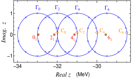
Figure 2: (Color online) Demonstration of the filter diagonalization for the yrast states of ⁴⁸Cr on the complex $z$-plane. The yrast-state energies obtained by the filter diagonalization and the Lanczos method are shown by crosses and small circles, respectively. For $J=0,2,4$ and 6, the COCG method is applied at $z=-32.0+0.1i$, $-31.0+0.1i$, $-30.0+0.1i$ and $-28.5+0.1i$ (in MeV), respectively (diamonds). The numerical integrations are carried out separately for each angular momentum using 10 points along the contour, which are shown by squares. Horizontal and vertical axes are real and imaginary parts of $z$, respectively.

Next we consider the low-lying excited states with $J=0$ and $T=0$ quantum numbers. In Fig. 3 (a) and (b), circles with $r=1$ and $r=2$ are shown, respectively, which cover the same energy interval [$-$33.5, $-$24.0] in MeV. In these calculations, we take the lowest state in 2p2h space as an initial state in Eq. (1).

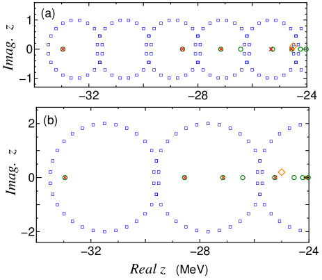
Figure 3: (Color online) Demonstration of the filter diagonalization for excited states of ⁴⁸Cr on the complex $z$-plane. The convention of symbols (crosses, circles, diamond and squares) is the same as that of Fig. 2. The energies located in [$-$33.5, $-$24.0] MeV are calculated using two integration contours with different radii, (a) $r=1$ MeV and (b) $r=2$ MeV. Horizontal and vertical axes are real and imaginary parts of $z$, respectively.

Figure 3 (a) is an extension of Fig. 2, for the $J=0$ state in wider energy regions. Numerical integration is carried out by 20 points for each circle, and we carry out the COCG calculation only at $z=24.5+0.1i$. For the other integral points, the values of the integrand are obtained by the shifted COCG method. For the circle with a center at $z=-30.7$ MeV, the moments vanish. It means no eigenvalue in this energy interval [$-$31.7, $-$29.7] in MeV. In the following circles, we can confirm the energies for $0_{1},0_{2},0_{3},$ and $0_{5}$ states. Because the initial state is $J=0$ and $T=0$ and matrix-vector multiplications in the COCG method conserve the quantum numbers, no state with different quantum numbers appears. Compared to the Lanczos method, the filter diagonalization is found to be advantageous with respect to the conservation of quantum numbers in numerical calculations.

In Fig. 3 (b), we use circles with radius $r=2$ MeV, which give us the same results. In this calculation, we use Eq. (15) for scaling. For both calculations, $0_{4}$ state is not reproduced because the initial state has very small components of the $0_{4}$ state (0.03%).

In Fig. 4, energy interval [$-$27.5, $-$22.5] in MeV is shown. Here we use smaller circles with $r=0.5$ MeV. Because a smaller circle includes fewer eigenvalues, it is easier to solve the equation. Smaller circles are expected to be useful when the level density is large. However, as shown in the next subsection, convergence of the COCG method unfortunately becomes slower.

In this calculation, as an initial state, we use the sum of the lowest five wave functions with $J=0$ and $T=0$ in the 2p2h space and can reproduce $0_{3\sim 9}$ states, including the $0_{4}$ state. As shown in Eq. (2), since Cauchy’s integral makes use of an initial state to extract eigenstates within the integration contour, the choice of the initial state is important.

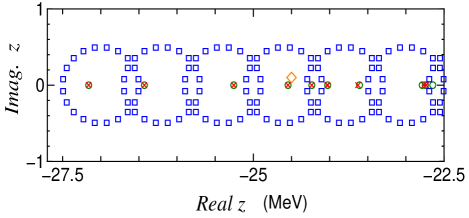
Figure 4: (Color online) Demonstration of the filter diagonalization for excited states of ⁴⁸Cr on the complex $z$-plane. The convention of symbols (crosses, circles, diamond and squares) is the same as that of Fig. 2. The energies located in [$-$27.5, $-$22.5] MeV are solved using integration contours with $r=0.5$ MeV. Horizontal and vertical axes are real and imaginary parts of $z$, respectively.

III.3 Convergence of the COCG method

The computational cost of the present method mainly depends on the convergence property of the COCG method. Due to the shifted COCG method, dependency on the number of integral points or the size of the integration contour is very weak. In Fig. 5, we show several convergence patterns of the COCG method at $z=-31+0.1i$, $-27+0.1i$ and $-23+0.1i$ (in MeV). Here the norm $|r|$ of the residual vector defined in Eq. (47) is plotted as a function of the number of iteration of the COCG method. We take $|r|/|b|<10^{-5}$ as a criterion of convergence, and as an initial state, we take the sum of the lowest five wave functions with $J=0$ and $T=0$ in the 2p2h space. In general, the convergence pattern of the COCG method is not monotonic, but on average, the norm of the residual vector decreases. As real part of $z$ increases, the number of iteration for convergence increases.

To investigate the $z$ dependence of the number of iteration, in Fig. 6, its contour plot on the complex $z$-plane is shown. The energy eigenvalues are also shown on the real axis by open circles. In general, as imaginary part of $z$ increases, the number of iteration decreases. As real part of $z$ increases, the number of iteration also increases. Along a given integration contour, the number of iteration of the COCG method becomes largest at the point $z$ whose real part is largest and imaginary part is smallest. Therefore, in Figs. 2$\sim$4, such a point is chosen as the $z_{0}$ of the COCG method, and the values at the other integral points are obtained by the shifted COCG.

Globally the COCG method converges fast for the ground and several low-lying states, while its convergence becomes worse for highly excited states. For such energy eigenvalues further theoretical development is necessary.

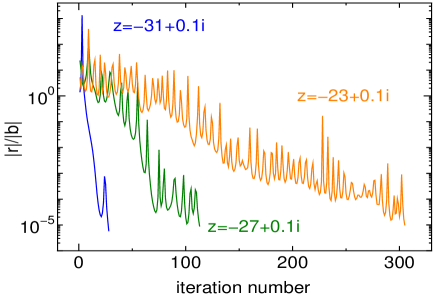
Figure 5: (Color online) Convergence patterns of the COCG method. The norm of residual vector is shown as a function of iteration number for $z=-31+0.1i$, $-27+0.1i$ and $-23+0.1i$ (in MeV).

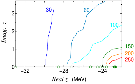
Figure 6: (Color online) Contour plot of the iteration number of the COCG method on the complex $z$-plane. Horizontal and vertical axes correspond to real and imaginary part of $z$, respectively. The energy eigenvalues are shown by open circles on the real axis.

III.4 Numerical accuracy

In the filter diagonalization, we use numerical integration to evaluate the energies and wave functions. Here we discuss their numerical accuracy. For example, we again consider the calculation of the ground state, taking the lowest state in the 2p2h space as an initial state. The ground-state energy is $-$32.954 MeV. Like Fig. 2, we enclose this energy pole by one circle with radius $r=1.0$ MeV. By moving its center position $\epsilon$, the ground-state energy pole is located at center or peripheral of the circle.

In Fig. 7 (a) and (b), we plot the moments $\mu_{0}$, $\mu_{1}$ and energy as a function of the center position $\epsilon$ for two cases of 10 and 30 integral points. Here $\mu_{0}$ is a square of an overlap between the initial 2p2h wave function and the ground state, and energy is given by the ratio of these two moments, $\mu_{1}/\mu_{0}+\epsilon$ because the integration contour encloses one energy pole. In Fig. 7 (b), the energy is quite constant as a function of the center position, although at $\epsilon=-32.954\pm 1.0$ MeV, the moments should be divergent, and for $\epsilon<-33.954$ MeV or $\epsilon>-31.954$ MeV, both $\mu_{0}$ and $\mu_{1}$ should be zero.

On the other hand, in Fig. 7 (a), we can see that each moment ill-behaves at such critical values. From Eq. (2), $\mu_{0}$ is constant and $\mu_{1}=(-32.954-\epsilon)\mu_{0}$. When the energy pole comes to the peripheral of the circle, $\mu_{0}$ deviates from a constant value and $\mu_{1}$ does not follow the linear behavior. By increasing the number of integral points, we can see that the numerical accuracy is improved. However, when the obtained energy is close to $\epsilon\pm r$, the energy itself may be still valid but the absolute values of the moments lose their reliability.

Next we consider the reliability of the calculation of wave functions. By using Eqs. (9) and (10), we can explicitly obtain wave functions. In Fig. 7 (c), we plot the overlap between the ground state wave functions obtained by the Lanczos method and by the filter diagonalization as a function of the center position. The overlap is also quite constant like energy. The ill-behavior comes from the denominator which can change the norm of wave functions. By renormalizing the wave function, this ill-behavior can be weakened. In Fig. 7 (c), the overlap between the initial state and the ground state obtained by the filter diagonalization is also quite constant. As this quantity is the same as $\mu_{0}$, the $\mu_{0}$ obtained from the wave function is more reliable. Thus in the filter diagonalization, the accuracy of energy and wave function is better than that of the absolute values of the moments.

Note that, by the energy variance $\sigma$ EXP defined as

$$\sigma=\frac{\langle H^{2}\rangle-\langle H\rangle^{2}}{\langle H\rangle^{2}},$$ (22)

we can evaluate the quality of the calculations without any references. In this case, this $\sigma$ is perfectly zero, which means that the obtained energy and wave function are exact. The computational cost of $\sigma$ is the same as that of the energy expectation value and this $\sigma$ can be easily numerically evaluated.

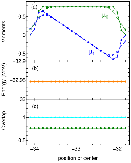
Figure 7: (Color online) The moments (a), energies (b) and overlaps (c) are plotted as a function of the center energy of integration contour, which is a circle with radius $r=1.0$ MeV. Two results for 10 and 30 integral points are shown by dotted lines with open circles and solid line with filled circles, respectively. In (b) and (c), two results are almost the same. In (c), upper line with marks (sky blue) shows overlaps between the ground states obtained by the Lanczos method and by the filter diagonalization. Lower line with marks (green) shows the same quantity as the $\mu_{0}$ but it is evaluated by the obtained wave functions.

III.5 Test of M1 strength function

As an accuracy test for the spectral strength functions obtained with the filter diagonalization, we consider an M1 strength function of ⁴⁸Cr.

The ground state $|\psi_{0}\rangle$ with $J=0$ and $T=0$ is obtained by the Lanczos method or the filter diagonalization. The M1 operator $O$ with the free g-factors is given as

$$O=g_{l}^{\pi}L^{\pi}+g_{l}^{\nu}L^{\nu}+g_{s}^{\pi}S^{\pi}+g_{s}^{\nu}S^{\nu}$$ (23)

where $L^{\pi}$ and $L^{\nu}$ are the proton and neutron orbital angular momentum operators and $S^{\pi}$ and $S^{\nu}$ are the proton and neutron spin operators, respectively. The free g-factors are $g_{l}^{\pi}=1$, $g_{l}^{\nu}=0$, $g_{s}^{\pi}=5.586$ and $g_{s}^{\nu}=-3.826$. We consider the $|\varphi_{0}\rangle=O|\psi_{0}\rangle$, of which angular momentum is 1, while the M1 operator $O$ mixes isospin. Then we classify the M1 operators as,

$$O=O^{T=0}+O^{T=1}$$ (24)

and

$$O^{T=0} = \displaystyle\frac{g_{l}^{\pi}+g_{l}^{\nu}}{2}(L^{\pi}+L^{\nu})+\frac{g_{s}^{\pi}+g_{s}^{\nu}}{2}(S^{\pi}+S^{\nu})$$ (25)

$$O^{T=1} = \displaystyle\frac{g_{l}^{\pi}-g_{l}^{\nu}}{2}(L^{\pi}-L^{\nu})+\frac{g_{s}^{\pi}-g_{s}^{\nu}}{2}(S^{\pi}-S^{\nu}).$$ (26)

As an initial wave function of the filter diagonalization, we prepare $|\varphi_{0}\rangle=O^{T=0}|\psi_{0}\rangle$ and $|\varphi_{0}\rangle=O^{T=1}|\psi_{0}\rangle$, of which angular momentum are 1 and isospin are 0 and 1, respectively. By this technique, the filter diagonalization is carried out within the specified space.

In Figs. 8 (a)-(c), we present several strength functions obtained by the double Lanczos method with different numbers of Lanczos iterations. Lower energy part of the strength function converges fast as a function of the number of Lanczos iterations, while convergence of higher energy part of the strength function is slow. In Fig. 8 (d), we present the results of the filter diagonalization. We can see that the present filter diagonalization can correctly reproduce the M1 strength function, compared to Fig. 8 (c).

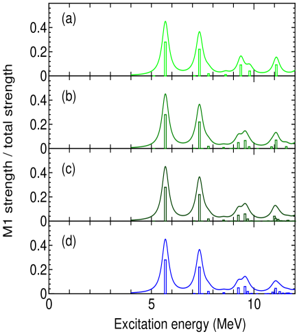
Figure 8: (Color online) The M1 strengths divided by the total strength as a function of excitation energy. The results are obtained by the double Lanczos method with (a) 50, (b) 100, (c) 500 iterations, while (d) by the filter diagonalization. The curves show the results of fits by a Lorentzian with a half width of 200 keV.

IV Conclusion

In this paper, based on the SS + shifted COCG method, we have shown an alternative diagonalization method for shell-model calculations. This method is called the filter diagonalization. It has a salient feature that eigenvalues and eigenstates can be searched for within a given energy interval. The filter diagonalization works equally well or is superior to the Lanczos method. Since both methods are based on the property of the Krylov space defined by eq.(54), their basic frameworks are similar. However, the following differences can distinguish one from the other.

In state-of-the-art large-scale shell-model calculations, the $M$-scheme is very useful but it needs a delicate treatment for angular momentum and isospin. In the numerical calculations, the robustness of conservation of these quantum numbers is different between the two methods. In the Lanczos method, small round-off errors easily break down such conservation, so that the double Lanczos method double was developed. On the other hand, in the filter diagonalization, conservation of the quantum numbers is found to be quite robust, which is a superior property. One of the problems in the Lanczos method, when applied to large-scale calculations, is reorthogonalization of the Lanczos vectors, which demands a heavy I/O access to storage devices. In the filter diagonalization, we use residual vectors, which are similar to the Lanczos vectors, but reorthogonalization is not necessary. This is another superior property. Because of the two merits, the filter diagonalization is superior to the Lanczos method especially for the calculations of excited states and spectral strength functions.

To examine such properties of the filter diagonalization, we have investigated its feasibility by taking ⁴⁸Cr as an example with the configuration space consisting of $f_{7/2}$, $p_{3/2}$, $f_{5/2}$, and $p_{1/2}$ orbits. This calculation is often considered as a touchstone of a new method aiming at large-scale shell-model calculations. We have demonstrated that while keeping good angular momentum and isospin, the filter diagonalization can obtain the yrast states and off-yrast states efficiently, and that it can also be useful for spectral strength functions. As for larger-scale calculations, we have tested the filter diagonalization for the case of ⁵⁶Ni with GXPF1A interaction GXPF1A . The 8p8h space horoini has approximately $2.5\times 10^{8}$ dimension. We can correctly obtain the ground state, oblate and prolate deformed states by the filter diagonalization.

Finally, we point out two open problems. One is the convergence of the COCG method, which depends on the position of complex energy $z$. For highly excited states, convergence becomes slow. The other is how to choose the integral contour and integral points for more efficient or unskilled computation. The present integral contour is circle but this is not unique QCD . Other integral contours may be more convenient and may solve the convergence problem. For these problems, further theoretical developments are strongly needed.

V Acknowledgment

The authors acknowledge Prof. M. Oi and Prof. Y. Sun for valuable comments about the manuscript. This research was supported in part by MEXT(Grant-in-Aid for Scientific Research: 21246018 and 21105502)

Appendix A Factorization of Hankel matrix

Here we summarize a factorization of the Hankel matrix. The moments are defined as

$$\mu_{p}=\sum a_{k}^{p}b_{k}$$ (27)

where $a_{k}$ and $b_{k}$ are, in general, complex numbers. The $n\times n$ Hankel matrix is defined as

$$N = \left(\begin{array}[]{cccc}\mu_{0},&\mu_{1},&\cdots&\mu_{n-1}\\ \mu_{1},&\mu_{2},&\cdots&\mu_{n}\\ \vdots&&\ddots&\vdots\\ \mu_{n-1},&\mu_{n},&\cdots&\mu_{2n-2}\end{array}\right)$$ (32)

$$= \left(\begin{array}[]{cccc}\Sigma b_{k},&\Sigma a_{k}b_{k},&\cdots&,\Sigma a_{k}^{n-1}b_{k}\\ \Sigma a_{k}b_{k},&\Sigma a_{k}^{2}b_{k},&\cdots&,\Sigma a_{k}^{n}b_{k}\\ \vdots&&\ddots&\vdots\\ \Sigma a_{k}^{n-1}b_{k},&\Sigma a_{k}^{n}b_{k},&\cdots&,\Sigma a_{k}^{2n-2}b_{k}\end{array}\right).$$ (37)

The $n\times n$ Vandermonde matrix $V$ and diagonal matrix $D$ are defined as

$$V^{T}=\left(\begin{array}[]{cccc}1,&a_{1},&\cdots&a_{1}^{n-1}\\ 1,&a_{2},&\cdots&a_{2}^{n-1}\\ \vdots&&\ddots&\vdots\\ 1,&a_{n},&\cdots&a_{n}^{n-1}\end{array}\right),$$ (38)

and

$$D=\left(\begin{array}[]{cccc}b_{1},&0,&\cdots&0\\ 0,&b_{2},&\cdots&0\\ \vdots&&\ddots&\vdots\\ 0,&0,&\cdots&b_{n}\end{array}\right).$$ (39)

Therefore, the following factorization holds as,

$$N=VDV^{T}.$$ (40)

Next we consider the matrix $M_{ij}=\mu_{i+j-1}$, which can be shown as

$$M=VD\Lambda V^{T},$$ (41)

where

$$\Lambda=\left(\begin{array}[]{cccc}a_{1},&0,&\cdots&0\\ 0,&a_{2},&\cdots&0\\ \vdots&&\ddots&\vdots\\ 0,&0,&\cdots&a_{n}\end{array}\right).$$ (42)

By these factorizations, we can prove SS1

$$M-\lambda N=VD(\Lambda-\lambda I)V^{T}.$$ (43)

Therefore, eigenvalues of generalized eigenvalue equation, $Mx=\lambda Nx$, are $\lambda=a_{k}(k=1,2,3,\cdots).$

Appendix B Shifted COCG method

The conjugate gradient (CG) method is an algorithm to numerically solve linear system as

$$Ax=b$$ (44)

where $A$ is a matrix and $x$ and $b$ are vectors. We consider the following quadratic function $f(x)$ defined as

$$f(x)=\displaystyle\frac{1}{2}x^{T}Ax-x^{T}b.$$ (45)

At the stationary point $x_{m}$, where $f^{\prime}(x_{m})=0$, the equation $Ax_{m}=b$ is satisfied. Therefore, we iteratively minimize $f(x)$ by changing $x$ along negative gradient direction, starting from $x_{0}$. A merit of the CG method is that we can handle only multiplication of matrix $A$ to vector $x$. During iteration process, matrix $A$ is unchanged and sparseness of matrix $A$ always holds. In the application of quantum systems, it is very useful for conservation of quantum numbers.

The complex orthogonal conjugate gradient (COCG) method COCG is a generalization of the CG method for complex, symmetric, but non-hermitian matrices. Its algorithm is shown by iterative relations among $x_{k},r_{k}$ and $p_{k}$ vectors ($k=1,2,3\cdots$) as,

$$x_{k+1}=x_{k}+\alpha_{k}p_{k},$$ (46)

$$r_{k+1}=r_{k}-\alpha_{k}Ap_{k},$$ (47)

$$p_{k+1}=r_{k+1}+\beta_{k}p_{k},$$ (48)

where $\alpha_{k}=r_{k}^{T}r_{k}/p_{k}^{T}Ap_{k}$ and $\beta_{k}=r_{k+1}^{T}r_{k+1}/r_{k}^{T}r_{k}$ ( Note that $\alpha_{k}\neq r_{k}^{\dagger}r_{k}/p_{k}^{\dagger}Ap_{k}$ and $\beta_{k}\neq r_{k+1}^{\dagger}r_{k+1}/r_{k}^{\dagger}r_{k}$). Initial conditions are $\alpha_{0}=1$, $\beta_{0}=0$, $x_{0}=0$ and $r_{0}=b$. As iteration number $k$ increases, the norm $|r_{k}|$ of residual vector $r_{k}$ decreases. The convergence criterion is given for $|r_{k}|/|b|$. If this convergence condition is fulfilled, we can obtain numerically approximated solution $x$.

Next we consider a series of shifted linear equations as

$$(A-\sigma I)x^{\sigma}=b,$$ (49)

where $\sigma$ is a complex number and $I$ is a unit matrix. If we start above iteration from $x_{0}=0$, the $k$-th residual vector $r_{k}^{\sigma}$ of the COCG method for Eq. (49) can be proven to be proportional to the $k$-th residual vector $r_{k}$ of the COCG method shiftedCOCG for Eq. (44) (i.e., Eq. (49) with $\sigma=0$);

$$r_{k}^{\sigma}=\displaystyle\frac{1}{\pi_{k}^{\sigma}}r_{k},$$ (50)

where $\pi_{k}^{\sigma}$ is a proportional coefficient and satisfies following iterative relations as,

$$\pi_{k+1}^{\sigma} = (1+\displaystyle\alpha_{k}\sigma)\pi_{k}^{\sigma}+\frac{\alpha_{k}\beta_{k-1}}{\alpha_{k-1}}(\pi_{k}^{\sigma}-\pi_{k-1}^{\sigma}),$$ (51)

$$\alpha_{k}^{\sigma} = \displaystyle\frac{\pi_{k}^{\sigma}}{\pi_{k+1}^{\sigma}}\alpha_{k},$$ (52)

$$\beta_{k}^{\sigma} = \left(\frac{\pi_{k}^{\sigma}}{\pi_{k+1}^{\sigma}}\right)^{2}\beta_{k}.$$ (53)

These iterative relations can be derived shiftedCOCG from an invariance property of two Krylov subspaces concerning Eqs.(44) and (49). The former Krylov subspace is generated by the iteration of the CG method, that is,

$$span\{b,Ab,A^{2}b,\cdots\}.$$ (54)

By shifting $A$ as $A-\sigma I$, the latter Krylov subspace becomes,

$$span\{b,\left(A-\sigma I\right)b,\left(A-\sigma I\right)^{2}b,\cdots\}.$$ (55)

This subspace is the same as that defined in (54).

References

- (1) C. Lanczos, J. Res. Nat. Bur. Stand, 45, 255 (1950).
- (2) E. Caurier, code ANTOINE, Strasbourg, 1989 (unpublished).
- (3) M. Horoi, B.A. Brown and V. Zelevinsky, Phys. Rev. C 67, 034303 (2003).
- (4) T. Mizusaki, RIKEN Accel. Prog. Rep. 33, 14 (2000).
- (5) T. Sakurai, H. Sugiura, J. Comput. Appl. Math. 2003, 159, 119.
- (6) T. Ikegami, T. Sakurai, U. Nagashima, Technical Report CS-TR-08-13, Tsukuba, 2008.
- (7) R. Takayama, T. Hoshi, T. Sogabe, S.-L. Zhang, T. Fujiwara, Phys. Rev. B 73, 165108 (2006).
- (8) B. Jegerlehner, hep-lat/9612014v1.
- (9) H. A. van der Vorst and J. B. M. Melissen, IEEE Trans. on Magnetics 26, 706 (1990).
- (10) M. Ogasawara, H. Tadano, T. Sakurai and S. Itoh, Trans. Japan SIAM, Vol. 14, No. 3 (2004) (in Japanese).
- (11) H. Ohno, Y. Kuramashi, T. Sakurai and H. Tadano, JSIAM Letters, in press.
- (12) T. Sakurai, J. Asakura, H. Tadano and T. Ikegami, JSIAM Letters 1 76 (2009). T. Sakurai, P. Kravanja, H. Sugiura and Marc Van Barel, J. Comput. Appl. Math. 152 (2003) 467.
- (13) R. R. Whitehead and A. Watt, J. Phys. G: Nucl. Phys. 4, 835 (1978).
- (14) We can also choose on the real axis. See Ref.QCD .
- (15) For instance, J. Engel, W. C. Haxton, and P. Vogel, Phys. Rev. C 46, R2153 (1992), Roger Haydock and Ronald L. Te, Phys. Rev. B 49, 10845 (1994).
- (16) E. Caurier and A. P. Zuker, A. Poves and G. Martinez-Pinedo, Phys. Rev. C 50, 225 (1994).
- (17) M. Honma, T. Mizusaki and T. Otsuka, Phys. Rev. Lett. 77, 3315-3318 (1996).
- (18) B. Thakur, S. Pittel and N. Sandulescu, Phys. Rev. C 78, 041303(R) (2008).
- (19) T. Mizusaki and M. Imada, Phys. Rev. C 65, 064319 (2002), Phys. Rev. C 67, 041301(R) (2003).
- (20) A. Poves and A. Zuker, Phys. Rep. 70, 235 (1981).
- (21) T. Mizusaki and M. Honma, unpublished.
- (22) M. Honma, T. Otsuka, B. A. Brown, and T. Mizusaki, Eur. Phys. J. A 25 Suppl. 1, 499 (2005).
- (23) M. Horoi, B. A. Brown, T. Otsuka, M. Honma, and T. Mizusaki, Phys. Rev. C 73, 061305(R) (2006).