X-ray Shadowing Experiments Toward Infrared Dark Clouds

Abstract

We searched for X-ray shadowing toward two infrared dark clouds (IRDCs) using the MOS detectors on XMM-Newton to learn about the Galactic distribution of X-ray emitting plasma. IRDCs make ideal X-ray shadowing targets of $3\over 4$ keV photons due to their high column densities, relatively large angular sizes, and known kinematic distances. Here we focus on two clouds near $30\arcdeg$ Galactic longitude at distances of 2 and 5$\,{\rm kpc}$ from the Sun. We derive the foreground and background column densities of molecular and atomic gas in the direction of the clouds. We find that the $3\over 4$ keV emission must be distributed throughout the Galactic disk. It is therefore linked to the structure of the cooler material of the ISM, and to the birth of stars.

1 Introduction

The diffuse X-ray background of the Milky Way has been studied for over 30 years and yet relatively little is known about the distribution of its emission in the Galactic plane. Most diffuse Galactic emission arises from $\sim 1-3\times 10^{6}$ K plasma (McCammon et al., 1983), but the origin and distribution of this plasma are still debated. Two factors are responsible for the difficulty in determining the distribution of this plasma: confusion and absorption. Confusion arises because one cannot determine the origin of an individual X-ray. Even though most X-rays contributing to the diffuse background of the Milky Way are thermal in origin and the spectra of this plasma show strong line emission, the available X-ray detector energy resolution is insufficient to provide velocity (and therefore distance) information. Thus it is very difficult to determine the true distribution of X-ray emitting plasma along a given line of sight.

Shadowing experiments are the only way to determine the distribution of hot plasma in the plane of the Milky Way. To date, they have been used primarily in the $1\over 4$ keV band to study the distribution of 0.1 keV plasma within the Local Hot Bubble and in the lower halo (e.g., Snowden et al., 2000). A few shadowing experiments at higher energy ($3\over 4$ keV and 1.5 keV) using ROSAT data (e.g., Park et al., 1997; Almy et al., 2000) have shown evidence for the existence of an extensive distribution of hot plasma well within the solar circle. This emission has been linked to the Milky Way X-ray bulge which has a scale height of $\sim 1.8$ kpc and a radial extent of $\sim 5$ kpc (Snowden et al., 1997), but there are likely additional components distributed throughout the Galactic disk.

Most studies of the X-ray background have focused on the Local Hot Bubble (LHB). The LHB is a region of about 100 pc in radius, surrounding the Sun filled with a hot, rarefied $10^{6}$ K plasma (e.g., Snowden et al., 1990). Beginning with Snowden, McCammon, & Verter (1993), many groups have effectively mapped the distribution of this gas (e.g. Smith et al., 2005; Galeazzi et al., 2007; Henley, Shelton, & Kuntz, 2007; Smith et al., 2007; Henley & Shelton, 2008). These studies have shown the utility of X-ray shadowing in mapping a large region of the sky at higher Galactic latitudes. Here we utilize similar techniques but extend the analysis to larger distances in the Galactic plane using dense molecular clouds.

Infrared Dark Clouds (IRDCs) are very dense molecular clouds that appear dark at infrared wavelengths. They are seen in absorption against the mid-IR background. IRDCs were first identified as a significant population in the Midcourse Space Experiment (MSX) mid-infrared data (Egan et al., 1998), and are a ubiquitous feature of the higher resolution Galactic Legacy Infrared Survey Extraordinaire (GLIMPSE: Benjamin et al., 2003). IRDCs have very high column densities of $10^{22}$ cm^-2 (Simon et al., 2006, hereafter S06), and possibly as high as $10^{23}-10^{25}$ cm^-2 (Egan et al., 1998; Carey et al., 1998). They exist at a wide range of distances and are most easily seen in the plane of the Galaxy (S06).

S06 found distances to 313 IRDCs using the Galactic Ring Survey of ${}^{13}{\rm CO}$ emission (GRS; Jackson et al., 2006) to establish a morphological match between the ${}^{13}{\rm CO}$ gas and the mid-infrared extinction. Using the rotation curve of Clemens (1985), S06 converted the velocity of the associated ${}^{13}{\rm CO}$ gas into a distance to the IRDC. In the inner Galaxy (the focus of the present study), every velocity has two possible distance solutions. IRDCs, however, are seen in absorption against the Galactic plane and therefore the near distance can be assumed.

IRDCs make ideal X-ray shadowing candidates. Their high column densities make them effective absorbers of background X-ray photons; X-ray emission from the direction of the IRDC must originate in the foreground. Thus, using IRDC absorption, one can separate foreground and background X-ray components. The distribution of IRDCs also spans a wide range of distances (see S06, Jackson et al., 2008). With enough X-ray absorption measurements of IRDCs along different lines of sight, an accurate map of the hot ISM may be created.

2 IRDC Sample

The present study includes two clouds from the catalog of S06 that have high column densities, large angular sizes, and are closely grouped on the sky. Our goal is to select clouds that would cause complete absorption of X-ray photons originating behind the cloud. The models given in Snowden et al. (1994) predict that a total column density of $1\times 10^{22}$ cm^-2 will absorb $\sim\,98\%$ of incident photons at $3\over 4$ keV. Column densities of $10^{22}$ are frequently found for IRDCs (see S06). To ensure sufficient counts in both the on– and off–cloud directions, the target IRDCs should cover approximately half the XMM-Newton detector. Our ideal situation is one in which there are multiple large clouds closely grouped on the sky but at various distances. The close grouping allows one to disentangle the emission components along a given line of sight.

The properties of the two IRDCs observed by XMM-Newton are summarized in Table 1. Listed are the IRDC name, the Galactic longitude and latitude, the angular size, and the molecular column density. All parameters in Table 1 are reproduced from S06. The two target clouds have high column densities, large angular sizes, and are near $l=30\arcdeg$.

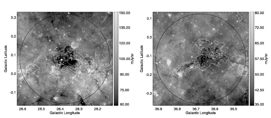
Figure 1: IRDCs shown in absorption against GLIMPSE 8µm emission. The left panel shows G28.37+0.07 and the right panel shows G36.67$-$0.11. The contours are ${}^{13}{\rm CO}$ integrated intensity from the GRS. Tick-marks on the contours point downhill, toward decreasing ${}^{13}{\rm CO}$ integrated intensity. The large black circles represent the XMM-Newton field of view ($\sim 30\arcmin$).

The mid-infrared emission of the two IRDC fields is shown in Figure 1. The background image in this figure is from the GLIMPSE 8µm survey (Benjamin et al., 2003) and the contours are ${}^{13}{\rm CO}$ integrated intensity from the GRS. We have created the integrated intensity map using the LSR velocity and line width from the S06 catalog. Tick-marks on the contours indicate the direction of decreasing ${}^{13}{\rm CO}$ integrated intensity. The large circle in this figure is approximately the XMM-Newton field of view ($\sim 30\arcmin$). Immediately evident in this figure is the excellent morphological match between the GRS ${}^{13}{\rm CO}$ contours and the strong mid-infrared extinction. The molecular clouds associated with the IRDCs take up a significant fraction of the XMM-Newton field of view. IRDC G28.37+0.07 is located at the center of a large, dense molecular cloud which is roughly ellipsoidal in projection. The two clouds are at very different distances, G28.37+0.07 lies $\sim 5$ kpc from the Sun and G36.67$-$0.11 lies $\sim 2$ kpc from the Sun (S06).

3 Observations and Data Reduction

Our clouds were observed by XMM-Newton on 2006 April 11 for 25 ks each (IRDC G28.37+0.07 with XMM-Newton ObsID 0302970301 and IRDC G36.67$-$0.11 with ObsID 0302970201).

One of us (SLS) has developed a powerful suite of PERL and FORTRAN scripts to analyze XMM-Newton extended source data called XMM-ESAS (Snowden et al., 2008). This software is based on the background modeling described in Snowden, Collier & Kuntz (2004) and Kuntz & Snowden (2008). The software currently only operates on the MOS detector data and subsequent to this analysis has been incorporated into the XMM-Newton mission Standard Analysis Software (SAS) package.

To remove intervals of high soft proton contamination, we must first temporally filter and clean the events file. The signature of soft proton contamination is a fluctuating light curve. The XMM-ESAS software creates a count rate histogram and fits a Gaussian to the peak of the histogram. In observations with minimal contamination, this histogram would appear Gaussian; a non-Gaussian shape to the distribution is also indicative of soft-proton contamination. The software defines count-rate intervals within $1.5\sigma$ of the median count rate as acceptable, and filters the events file to remove intervals that do not satisfy this criterion. While effective at removing intermittent contamination, this process does not remove consistent low-level contamination that is also likely present. The light-curve for G28.37+0.07 is quite steady and almost all the data are useable. The light-curve of G36.67$-$0.11, however, indicates a high level of soft proton contamination and only $\sim 20\%$ of the observation time is usable.

4 Estimation of Column Density

An estimate of the total column density to each IRDC can drastically improve the reliability and accuracy of the X-ray spectral fitting. Above 0.5 keV, the most significant source of X-ray absorption is metals. With normal abundances, the total X-ray opacity should be proportional to $N({\rm H})+2N({\rm H_{2}})$. Thus, we estimate the molecular column density using the ${}^{13}{\rm CO}$ emission from the GRS, and estimate the atomic column density using the 21 cm H i VLA Galactic Plane Survey (VGPS: Stil et al., 2006).

Our spectral fitting procedure treats the on– and off–cloud spectra separately (as do all X-ray shadowing experiments). This is the only way one can separate components of the X-ray background that originate in front of the cloud from those that originate behind it. One must therefore compute on– and off–cloud column densities separately. We do this by first defining the on– and off–cloud regions.

One of us (LDA) has developed an astronomical software program in IDL. This software allows one to define regions of interest in an image using a threshold selection tool. The user can vary the threshold upwards or downwards to define smaller or larger regions. The output of this thresholding selection, the x and y positions of the data points on the threshold boundary in sky coordinates, can then be converted to detector coordinates within the software, as is appropriate for analysis in the XMM-Newton Science Analysis Software (SAS). This conversion employs the SAS program edet2sky repeatedly for each coordinate pair to convert from a region in sky coordinates to a region in detector coordinates.

Using our IDL software, we define the on–cloud region as the sky positions possessing both high mid-infrared extinction and high ${}^{13}{\rm CO}$ column density. Our goal is to create a region large enough to have sufficient counts in the on–cloud region for good statistics. Ideally, the on– and off–cloud regions would each cover half the XMM-Newton field of view. The off–cloud region encompasses all locations in the XMM-Newton field of view not including the on–cloud region. The on–cloud region roughly corresponds to the largest contour in Figure 1.

4.1 Molecular Column Density

We must separate the total molecular column density into a component foreground to the IRDC and a component beyond the IRDC. We therefore must estimate the distances to the molecular gas clumps that contribute to the column density in the XMM-Newton field of view. In the first Galactic quadrant (where the target IRDCs lie), each radial velocity has two possible distance solutions, a “near” and a “far” distance. This problem is known as the kinematic distance ambiguity (KDA). Gas along the same line of sight as an IRDC could lie either in front of or behind the cloud. This problem is illustrated in Figure 2 for IRDC G28.37+0.07. Figure 2 shows the loci of distances from the Sun corresponding to a particular velocity, assuming the Galactic rotation curve of Clemens (1985). The two-fold distance degeneracy is clearly shown. Because IRDCs are seen in absorption, we assume they lie at the near distance. The cloud velocity of 78.6 $\,{\rm km\,s}^{-1}$ places G28.37+0.07 at a distance of 4.8 $\,{\rm kpc}$ from the Sun. Any gas with a velocity greater than 78.6 $\,{\rm km\,s}^{-1}$ must lie beyond the cloud. Molecular gas at velocities less than 78.6 $\,{\rm km\,s}^{-1}$, however, could lie at either the near or the far distance.

H i self-absorption (H i SA) can remove the distance ambiguity of the molecular gas clumps in the XMM-Newton field of view. This technique relies on cold foreground H i absorbing the emission of warm background H i at the same velocity. Warm H i is ubiquitous in our Galaxy and emits at all allowed velocities. Litzt, Burton & Bania (1981) hypothesized that molecular clouds must contain H i, a result which has been confirmed in numerous subsequent observations (e.g., Kuchar & Bania, 1993; Williams & Maddalena, 1996). This small population of cold neutral H i atoms inside molecular clouds is maintained by interactions with cosmic rays. The H i inside molecular clouds at the near distance will produce an absorption signal because there is ample warm H i emitting at the same velocity at the far distance. Any cloud at the far distance should not show H i SA because there is no background H i emitting at the same velocity. H i SA is therefore a general technique for finding distances to molecular clouds. This technique was shown by Jackson et al. (2002) to be effective at resolving the KDA for a dense molecular cloud, by Busfield et al. (2006) for resolving the KDA for young stellar objects, and by Anderson & Bania (2009) for resolving the KDA for the molecular gas associated with H ii regions, and by Roman-Duval et al. (2009) for resolving the KDA for GRS molecular clouds.

We utilize the procedure outlined in Simon et al. (2001) to convert from GRS ${}^{13}{\rm CO}$ emission line parameters into an estimate of column density. This procedure assumes a standard CO excitation temperature of 10 K. The conversion equation is:

$$N({\rm H_{2}})=5.2\times 10^{20}\,T\Delta V\,[{\rm cm^{-2}}]\,,$$ (1)

where $T$ is the main beam line intensity in degrees Kelvin and $\Delta V$ is the line width in $\,{\rm km\,s}^{-1}$. The column density found using this procedure is accurate to within a factor of $\sim 2$ due to uncertainties in the conversion from ${}^{13}{\rm CO}$ to ${\rm H_{2}}$.

To find the molecular column densities for both on– and off–cloud directions, we calculate the column density of all significant ${}^{13}{\rm CO}$ molecular clumps in the XMM-Newton field of view by first fitting Gaussians to the average on– and off– cloud GRS spectra. We transform the line parameters derived from these Gaussians into column densities using Equation 1. The application of Equation 1 computes the total column density along each line of sight, but gives no information about whether the components lie at the near or the far distance. By examining the average ${}^{13}{\rm CO}$ and H i spectrum of each molecular clump in the XMM-Newton field of view for H i SA, we determine whether the near or the far distance is appropriate for each molecular clump. We assign the column densities of the molecular clumps found to lie in front of the target cloud to the foreground component, and the column densities of the molecular clumps found to lie behind to the target cloud to the background component.

4.2 Atomic Column Density

We use a similar procedure to calculate the H i column density using the VGPS. The conversion to H i column density employs the equation:

$$N({\rm H\,I})=1.82\times 10^{18}\ T_{\rm s}\int\tau(v)\,{\rm d}v\,[{\rm cm^{-2}}]\,,$$ (2)

where $T_{\rm s}$ is the H i spin temperature in degrees Kelvin, and $v$ is given in $\,{\rm km\,s}^{-1}$. For H i, the spin temperature is much less well constrained compared to the excitation temperature of ${}^{13}{\rm CO}$. A good average value between the hot and cool H i components is 150 K (see Dickey & Lockman, 1990, and references therein). Equation 2, requires an estimate of the optical depth for the H i line using the equation:

$$\tau_{\rm HI}=-{\rm ln}\left(1-\frac{T_{\rm L}}{T_{\rm s}-T_{\rm BG}}\right)\,,$$ (3)

where $\tau_{\rm HI}$ is the optical depth of H i, $T_{\rm L}$ is the H i line intensity, $T_{\rm s}$ is the H i spin temperature, and $T_{\rm BG}$ is the intensity from background sources. The largest source of background emission is the cosmic microwave background; because it produces a negligible effect at 21 cm, we ignore its contribution here. Assuming a spin temperature of 40 K lowers our calculated column densities by a factor of $\sim 2$.

For H i  there is less information about whether the gas originates in front of or behind the cloud compared to CO. As we did for ${}^{13}{\rm CO}$, we compute average on– and off–cloud spectra. A typical H i spectrum does not show distinct, clean lines. We therefore compute the area under the curve directly, instead of fitting Gaussians, and convert this to H i column density using Equations 2 and 3. We assume that the H i is uniformly distributed along the line of sight to a distance of 15 kpc from the Sun and split the column density distribution into foreground and background components, weighted by the distance to the cloud. For example, we assume G28.37+0.07 (at a distance of 5 kpc) has 33% of the total H i along the line of sight in the foreground component, and 67% in the background component. Our values for the total H i column density are in very good agreement with those in the the Leiden/Argentine/Bonn H i survey (Kalberla et al., 2005) and the H i survey of Dickey & Lockman (1990) as found using the HEASARC online tool.

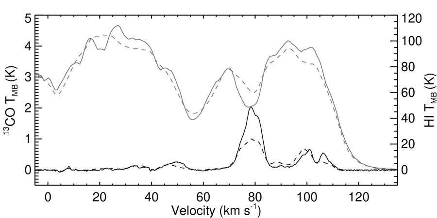
Figure 3: Average on–(solid curves) and off–cloud (dashed curves) spectra of H i (gray curves) and ${}^{13}{\rm CO}$(black curves) for G28.37+0.07.

Figure 3 shows the average on– (solid curves) and off–cloud (dashed curves) spectra of ${}^{13}{\rm CO}$ (black curves) and H i (gray curves) for Figure 3. For G28.37+0.07, H i absorption is seen at the velocity of all ${}^{13}{\rm CO}$ components with velocities less than the cloud velocity of 78.6 $\,{\rm km\,s}^{-1}$(this is clearer when analyzing each clump individually). Therefore, we assign all ${}^{13}{\rm CO}$ emission not associated with G28.37+0.07 that has velocities less than 76.6 $\,{\rm km\,s}^{-1}$ to the near component. We assign all ${}^{13}{\rm CO}$ features with velocities greater than 78.6 $\,{\rm km\,s}^{-1}$ to the far component. Also evident in Figure 3 is the strong H i absorption at the cloud velocity, which shows clearly that the cloud is at the near distance. The H i emission is less strongly peaked than the ${}^{13}{\rm CO}$ emission.

The results of our column density modeling are summarized in Table 2. This table gives the column density of atomic hydrogen, $N({\rm H})$, molecular hydrogen $N(\rm H_{2})$, and the total column density, $N_{\rm Total}=N({\rm H})+2N(\rm H_{2})$ in units of $10^{22}$$\,{\rm cm^{-2}}$ for G28.37+0.07 and G36.67$-$0.11. The contributions to the column density are given for the foreground and background components for the on– and off–cloud directions. The background component includes the contributions from the IRDCs themselves.

5 Spectral Analysis

Using our cleaned events files, we extract the X-ray spectra for both the on– and off–cloud regions in preparation for spectral fitting. Our on– and off–cloud regions are defined as before and correspond to high infrared extinction and high ${}^{13}{\rm CO}$ column density. We extract spectra from both MOS detectors and create auxiliary response files (ARFs), redistribution matrix files (RMFs), and background spectra. We increase the signal to noise by binning these spectra so there are at least 20 counts per spectral channel. We use XSPEC V11.3.2 (Arnaud et al., 1996) for the spectral analysis.

For the spectral fits, we assume the emission can be described as:

$$I_{X}=SP+I_{LHB}+I_{F}+I_{B}+(I_{R}+AGN)\,,$$ (4)

where $I_{X}$ is the measured X-ray flux, $SP$ is the contribution from soft proton contamination, $I_{LHB}$ is the emission from the LHB, $I_{F}$ is the Galactic X-ray emission foreground to the cloud, $I_{B}$ is the Galactic X-ray emission background to the cloud, $I_{R}$ is the emission from the Galactic ridge, and $AGN$ is the X-ray background from unresolved active galactic nuclei. There are three column density parameters in our models, one associated with $I_{F}$, one with $I_{B}$, and one with both $I_{R}$ and $AGN.$ The fitted column density associated with $I_{B}$ is poorly constrained (see below), which is why we do not treat the column density associated with $I_{R}$ and $AGN$ as the sum of that affecting $I_{F}$ and $I_{B}$. Below we describe in more detail the various model components we use to model the X-ray background and to separate foreground from background emission.

There are two main sources of contamination in our spectra. First, there is residual soft proton contamination not removed through time filtering ($SP$ in Equation 4). This component should have a power law distribution of energies, so we model its emission using the XSPEC model pow/b. This XSPEC component models a power-law noise distribution not folded through the instrument response. Secondly, there are two fluorescent instrumental lines of Al K$\alpha$ and Si K$\alpha$ near 1.6 keV. We assume a Gaussian shape for these lines and fit them explicitly.

Our models include three components for the X-ray background, as in Snowden et al. (2000). Along each line of sight, first there is $\sim 0.1$ keV emission from the LHB (Smith & Cox, 2001), $I_{LHB}$. We fit the the LHB emission with the XSPEC model apec (Smith et al., 2001), which represents collisionally-ionized diffuse plasma. Next, we assume that there are two components of the X-Ray background emission in the Galactic plane: one soft ($\lesssim$ 1 keV) and one hard (few keV), $I_{R}$. For these components we use the XSPEC model wabs $\times$ apec, which represents collisionally-ionized diffuse plasma attenuated by material along the line of sight. The soft component itself can be divided into two sources: emission in front of the IRDC, $I_{F}$, and emission from beyond the IRDC, $I_{B}$. Finally, there is extragalactic emission from unresolved AGN in the field, $AGN$. We model the contribution from AGN using a power law model with absorption, wabs $\times$ pow, where the power law index is set to $\alpha=1.46$ (Chen et al., 1997). This is expected to be the dominant component above 1 keV (Lumb et al., 2002).

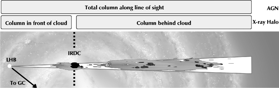
Figure 4: Components of the X-ray background attenuated by the Galactic column density for G28.37+0.07. The column density Molecular gas from the GRS is shown black while atomic gas from the VGPS is shown in gray. The Local Hot Bubble (labeled LHB), the direction of our observation (white wedge) and the direction towards the Galactic center are also shown. The size of the wedge and the LHB are slightly exaggerated for clarity. IRDC G28.37+0.07 is associated with a large dense molecular cloud 5 kpc from the Sun.)

We show the model components and the column densities affecting them graphically in Figure 4 for G28.37+0.07. In this figure, molecular gas is displayed in black and atomic gas is displayed in gray. The white wedge is an exaggerated representation of the XMM-Newton field of view. Also shown on the figure are the location of IRDC G28.37+0.07, the LHB, and the direction to the Galactic center (GC). The LHB size in the figure is exaggerated for clarity. Figure 4 shows that the AGN X-ray emission is affected by the total Galactic column density.

During the spectral modeling, we fit the spectra for each cloud simultaneously to improve the fit quality. We fix the abundance to Solar and use the Solar relative metal abundance of Anders & Grevesse (1989). We have five spectra for each cloud: on– and off–cloud spectra for both MOS detectors, as well as a ROSAT All Sky Survey (RASS; Snowden et al., 1997) spectrum derived from the HEASARC X-ray Background Tool. The RASS spectrum helps constrain the cosmic background at lower energies where the XMM-Newton detectors are less sensitive. We extract the RASS spectra from regions centered on our clouds of radius $0.5\arcdeg$ and normalize the spectra to 1 arcminute². We use the same RASS spectrum for the on– and off–cloud regions, but scale the emission by the relative area of these regions. We link the normalizations and temperatures of each spectral component for all five spectra to constrain the fits. We also link the temperature of the soft foreground component to that of the soft background component.

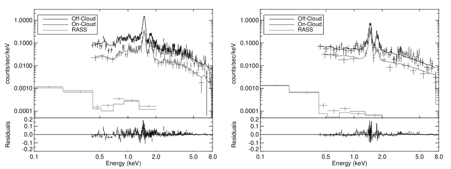
Figure 5: Spectral data and models for G28.37+0.07 (left panel, column density free fit) and G36.67$-$0.11 (right panel) from the MOS1 detector. Shown are the on–cloud (black), off–cloud (dark gray), and RASS (light gray) spectra. The bottom section of each panel shows the fit residuals.

The results of our spectral fitting procedure are shown in Figure 5 for the MOS1 detector. In Figure 5, the top curve is the on–cloud spectrum, and the lower curve is the off–cloud spectrum. The bottom curve is the RASS spectrum. The two prominent emission lines are the fluorescent instrumental lines of Al K$\alpha$ and Si K$\alpha$. The left panel of Figure 5 shows the spectra and model for G28.37+0.07, and the right panel shows the same for G36.67$-$0.11. It is evident from this figure that our model adequately fits the data. Also apparent from Figure 5 are the decreased counts for G36.67$-$0.11 due to the soft proton contamination. This results in greater uncertainty in the spectral fits.

For G28.37+0.07, we run our fits in two trials, once with the column densities fixed to their calculated values (see §4) and once with the column densities allowed to vary (hereafter the “fixed” and “free” trials). We allow the column densities to vary up to 100% from our calculated values to account for uncertainties in converting line parameters to column densities. Due to insufficient counts, we are unable to allow the column densities to vary for G36.67$-$0.11, and thus we run the spectral fits only with fixed values.

5.1 Spectral Fit Results

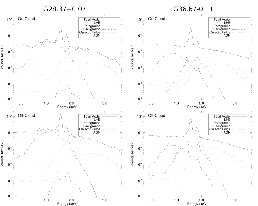
Figure 6: Model spectral components from the XSPEC fit to the on–cloud (top panels) and off–cloud (bottom panels) spectra for G28.37+0.07 (left panels) and G36.67$-$0.11 (right panels) from the MOS1 detector. For G28.37+0.07, the models are from the trial with column density free.

The results of our spectral fits are shown in Figure 6 and listed in Table 3. Figure 6 shows the best fit model components for G28.37+0.07 (left panels) and G36.67$-$0.11 (right panels). The top panels show the models for the on–cloud directions, and the bottom panels show the same for the off–cloud directions. The models for G28.37+0.07 are from the free trial. Table 3 lists the fitted temperature and emission measure (EM = $\int n_{e}^{2}dl$) for our four spectral model components, the reduced $\chi^{2}$ value, and the number of degrees of freedom in the fit. Errors in the table represent 90% confidence levels. Below we discuss the model components individually.

5.1.1 Column Densities

When allowed to vary, the column densities for G28.37+0.07 fit to similar, but generally lower, values compared to our calculated values (see §4). For the on–cloud spectra, the column density fits to $1.2^{+0.03}_{-0.02}\times 10^{22}$ $\,{\rm cm^{-2}}$ for the foreground component; we estimated $1.3\times 10^{22}$ $\,{\rm cm^{-2}}$. The column density background to the cloud is unconstrained when allowed to vary as its normalization fits to zero (see §5.1.4 below). The total column density affecting the Galactic ridge and AGN emission fits to $3.9^{+0.6}_{-0.5}\times 10^{22}$ $\,{\rm cm^{-2}}$ for the on–cloud spectra; we estimated $5.2\times 10^{22}$ $\,{\rm cm^{-2}}$. Thus, since the total column density affecting the Galactic Ridge and AGN component is the sum of that foreground and background to the cloud, we find $2.6\times 10^{22}$ for the background component. For the off–cloud spectra, the column density fits to $1.1^{+0.04}_{-0.03}\times 10^{22}$ $\,{\rm cm^{-2}}$ foreground to the cloud and to $2.9^{+0.3}_{-0.2}\times 10^{22}$ $\,{\rm cm^{-2}}$ for the total column density; we estimated $0.9\times 10^{22}$ $\,{\rm cm^{-2}}$ and $4.2\times 10^{22}$ $\,{\rm cm^{-2}}$, respectively.

Perhaps the most important column density parameter – the difference in column density between the on- and off–cloud regions – is the same in the fixed and free trials for G28.37+0.07: $1.0\times 10^{22}$ $\,{\rm cm^{-2}}$, although with a formal error derived from the fit of about 50%. The other discrepancies are discouraging, although the differences have little affect on the other model parameters. The largest effect can be seen in the emission measure of the foreground soft component (see below). Despite our care taken in estimating the column densities, errors in the conversion from ${}^{13}{\rm CO}$ line parameters to hydrogen column density are large and currently unavoidable. Longer or more sensitive observations are required to more accurately disentangle the competing effects of absorption from the Galactic column density and emission from the X-ray background.

5.1.2 LHB Component

The fixed and free column density trials for G28.37+0.07 both result in a LHB component temperature $kT=0.11$ keV (log$T$/K = 6.11). For G36.67$-$0.11, the LHB component fits to a temperature of 0.089 keV(log$T$/K = 6.02. These temperatures for the LHB component are in good agreement with that found by many previous studies (see Snowden et al., 1998, 2000; Kuntz & Snowden, 2000; Henley, Shelton, & Kuntz, 2007). The emission measure for the LHB component is less than what has been found by previous authors. We calculate an emission measure of $5.5\times 10^{-4}$ cm^-6 pc for the fixed trial and $5.4\times 10^{-4}$ cm^-6 pc for the free trial for G28.37+0.07. For G36.67$-$0.11, it is slightly higher: $6.3\times 10^{-4}$ cm^-6 pc. These values are three times less than that found by Henley, Shelton, & Kuntz (2007), $\sim 10$ times less than that found by Smith et al. (2007). This emission measure is in large part determined from the RASS 1/4 keV band data, and as the directions lie in the Galactic plane the surface brightness, and therefore the emission measure of the RASS data are relatively low.

5.1.3 Soft Foreground Component

The soft component fits to a temperature of 0.29 keV (log$T$/K = 6.53) in the fixed trial and to 0.30 keV (log$T$/K = 6.54) in the free trial for G28.37+0.07. For G36.67$-$0.11, the soft component is not very well constrained. In fact, the only constraint we can place on this component is that it is less than 0.35 keV(log$T$/K = 6.61). Kuntz & Snowden (2008) find a similar temperature for this component: 0.24 keV.

5.1.4 Soft Background Component

For the fixed trial of G28.37+0.07, the soft background component has little effect on the model. In fact, its removal has no impact on the quality of the fits, nor any impact on the value of the other parameters. The large column density in front of the background component causes significant absorption. The negligible effect this component has on our total model can be seen in Figure 6. For the free trial, the normalization for this component fits to zero. For G36.67$-$0.11, the soft foreground component and soft background component have similar intensities. The difference between the fits seen in Figure 6 for the two clouds is due partly to the decreased column density to G36.67$-$0.11. Perhaps a larger factor, however, could be the greater uncertainty in the spectral fits for G36.67$-$0.11 due to soft proton contamination.

5.1.5 Galactic Ridge Component

The temperature for the warm Galactic ridge component fits to 1.61 keV (log$T$/K = 7.27) in the free trial and to 2.34 keV (log$T$/K = 7.43) in the fixed trial for G28.37+0.07. This is a significantly higher than what has been found by previous authors. Kuntz & Snowden (2008) find a temperature of 0.71 keV for this component, with rather large error bars. Because of the decreased counts in the observation of G36.67$-$0.11, we were forced to fix the Galactic ridge component to the temperature found for G28.37+0.07. When allowed to vary, this component would fit to an extremely high temperature ($>10\,{\rm keV}$), which we deem unphysical, especially considering the results for G28.37+0.07.

Figure 6 shows that for both clouds the Galactic ridge emission is the strongest component of the model between 2 and 5 keV. To determine if this component is required by the spectral fits, we remove the hard component from the models for G28.37+0.07. Its exclusion results in significantly worse fits: the reduced $\chi^{2}$ value increases from 1.11 to 1.41. An F-test reveals that the inclusion of the Galactic ridge component is significant at the $15\sigma$ level. We conclude that this is a necessary component of our spectral fits although its temperature is not very well constrained.

5.2 O VII and O VIII Emission

Oxygen is the most abundant line-emitting element at the temperatures of the LHB. In a million degree plasma, oxygen is primarily in the O⁺⁶ state (O vii), and the strongest lines detectable by XMM-Newton are near 0.5 keV. The emission from other charge states (most important for our purposes is O viii) can be used as a diagnostic to constrain the temperature of the LHB and verify the temperature found previously through spectral fitting. There are three lines of O vii that are all near 0.57 keV, and there is a Ly$\alpha$ transition of O viii at 0.65 keV.

We measure the intensities of the O vii and O viii emission from the LHB by replacing the apec model component with a vapec model. The vapec model is identical to the apec model except that the atomic abundances may be individually modified. We set the oxygen abundance to zero and add two Gaussians representing the O vii and O viii emission lines at 0.57 keV and 0.65 keV. For G28.37+0.07, when we fix all the model parameters to their previously fit values (except for the vapec temperature and normalization), we find that the O vii line has an intensity of 3.4${}^{+0.4}_{-1.0}$ photons cm^-2 s^-1 sr^-1 (hereafter line units, LU). The vapec temperature fits to a value of 0.098 keV. When we fix the vapec temperature to the LHB temperature found previously, 0.11 keV, we find an O vii intensity of 3.3${}^{+0.7}_{-0.8}$ LU. We do not detect the O viii line in either of these trials. The same procedure applied to G36.67$-$0.11 yields similar results. With the vapec temperature allowed to vary, the O vii intensity is $1.9^{+1.3}_{-1.6}$ LU. The vapec temperature fits to 0.085 keV. When fixed to the 0.089 keV value found previously, the O vii intensity is $2.1^{+1.3}_{-1.3}$ LU. We do not detect the O viii line.

Our values for the O vii and O viii lines are in rough agreement with what has been found by other authors. In a shadowing experiment to a nearby ($\sim 200$ pc) filament, Henley, Shelton, & Kuntz (2007) found $3.4^{+0.6}_{-0.4}$ LU for the O vii line and did not detect the O viii line. Kuntz & Snowden (2008) found $1.75\pm 0.7$ LU for the O vii emission at (l,b) = ($111\hbox{$.\mkern-4.0mu^{\circ}$}14,1\hbox{$.\mkern-4.0mu^{\circ}$}11$). In a shadowing experiment of MBM 12, a high latitude cloud $\sim 50$ to $\sim 300$ pc distant, Smith et al. (2005) found $1.79\pm 0.55$ LU for O vii and $2.34\pm 0.36$ LU for O viii. They note that this unusually strong O viii emission can be explained by solar wind charge exchange (SWCX) contamination in their spectra. The SWCX emission is caused by electron transitions between neutral atoms and highly ionized species in the solar wind. It has a potentially large effect in X-ray data, especially following a coronal mass ejection event. Snowden, Collier & Kuntz (2004) showed the large effect on the oxygen lines that SWCX emission can have. In a followup study of MBM 12 with Suzaku, Smith et al. (2007) found $2.34\pm 0.33$ LU for O vii and $0.77\pm 0.16$ LU for O viii line emission. Using the X-ray Quantum Calorimeter aboard a sounding rocket, McCammon et al. (2002) found $4.8\pm 0.8$ LU for the O vii emission and $1.6\pm 0.4$ LU for the O viii emission.

While consistent with previous values, we note that there is likely some residual contamination from SWCX in our measured oxygen line intensities. Using the models in Smith et al. (2005), we estimate that for the EM and $T$ found here for the LHB, we should expect O vii and O viii intensities of $\sim 2$ and $<1$ LU, respectively. This indicates that the line intensities measured here cannot be solely due to a plasma in thermal equilibrium.

A consensus appears to be emerging that most of the O vii emission arises from the LHB (with a contribution from SWCX). Strong O viii emission, however, cannot arise from the LHB as this would imply a temperature inconsistent with other determinations. This emission must arise from SWCX (Snowden, Collier & Kuntz, 2004) or from a cool component distributed throughout the Galaxy (Kuntz & Snowden, 2008), likely with contributions from both sources. Our results are consistent with this interpretation. That we do not detect the O viii line is not surprising given the large absorbing column density and low expected line strength.

6 Image Analysis

We produce exposure corrected, background subtracted X-ray images to verify the results from the spectral analysis, and to search for a morphological match between the molecular emission and an X-ray decrement. Using the XMM-ESAS software, we create these images in three energy bands: 0.35–1.25 keV, 1.25–2.00 keV, and 2–10 keV. We model two sources of background in our images: the particle background and residual soft proton contamination. These background components must be removed as cleanly and completely as possible to ensure accurate results.

Using the filter-wheel-closed data, the XMM-ESAS software models the particle background (see Kuntz & Snowden, 2008). These data are dominated by the instrumental background because the chips were not exposed to the sky. We do not include blank sky data in the modeling of either the particle background nor the soft proton contamination. The blank sky files may suffer from residual soft proton contamination and solar wind charge exchange. Additionally, the blank sky files contain the cosmic background which we are attempting to observe. Using these data would not only add error to our models, but would also remove the signal of interest.

The XMM-ESAS software also allows for the creation of a model image of any residual soft proton contamination. Kuntz & Snowden (2008) characterize the reasonable ranges of the variations in both the spectrum and in the spatial distribution over the detectors. XMM-ESAS incorporates this characterization in the model soft proton image. The energy distribution of the soft proton contamination is determined from the power law index and normalization found in the spectral fits. For this input, we use the values found in the spectral fitting.

We subtract the model background and soft proton images, combine the data from the two MOS detectors and smooth the resultant image. The result of these operations is an exposure corrected, background subtracted image. The strongest X-ray shadow should be present in the 0.35–1.25 keV image. We show in Figure 7 the exposure corrected, background subtracted image for the 0.35-1.25 keV band of G28.37+0.07 (left panel) G36.67$-$0.11 (right panel). In the images of both clouds there is some indication of a shadow, but it not the clearly defined shadow one would expect, nor does it have the same depth one would expect. Furthermore, the same shadow that appears in the 0.35–1.25 band also appears in the 2.0–8.0 keV band. As there should not be strong absorption in the 2.0–8.0 keV band, this indicates that the “shadow” is a product of the detector, and not of the cloud itself. We conclude that the imaging analysis supports the spectral analysis and finds no X-ray shadow of the cooler component to the X-ray background.

7 Summary

We have conducted X-ray shadowing experiments on two infrared dark clouds near $l=30\arcdeg$ at distances of 2 and 5 kpc from the Sun to determine the spatial distribution of the X-ray background. We used H i and ${}^{13}{\rm CO}$ data to calculate the total atomic and molecular column densities for both the on– and off–cloud directions. Both clouds have very high proton column densities of $\gtrsim 4\times 10^{22}\,{\rm cm^{-2}}$. This high column density should absorb nearly all the soft background X-ray flux. We find that the cool, diffuse X-ray background must originate foreground to the clouds, within a few kpc of the Sun. Our results are further evidence that X-ray emitting plasma is distributed throughout the disk of our Galaxy (see Park et al., 1997; Kuntz & Snowden, 2008).

We found that the X-ray background is best fit with a three component model with contributions from the Local Hot Bubble (LHB), a soft component, and a hot component from the Galactic ridge. The LHB emission is best fit with a value of $\sim 0.1$ keV (log $T$/K = 6.06) for both clouds, in agreement with what has been found in previous studies. The soft component is best fit with a temperature of $\sim 0.3$ keV (log $T$/K = 6.54). This is the dominant source of emission between 0.7 and 1.0 keV. The Galactic ridge component is best fit with a temperature of 2 keV. This is the dominant source of emission in our spectral models between 2 and 5 keV. Our spectral fits show that most significant emission below $\sim 0.7$ keV can be attributed to the LHB (and/or to SWCX). Image analysis including accurate modeling of any background components failed to reveal an X-ray shadow, supporting the results of the spectral modeling.

We detect the O vii line for both clouds at levels of $\sim\,3$ photons cm^-2 s^-1 sr^-1. This intensity is $\sim 50\%$ higher than what one would expect from a thermal plasma with the emission measure and temperature of the LHB, indicating some level of contamination from solar wind charge exchange. These values are roughly in agreement with what has been found in previous studies. We do not detect the O viii line for either cloud.

Figure 2: Velocity versus distance plot for G28.37+0.07 showing the kinematic distance ambiguity. This cloud lies at the near distance of 4.82 kpc.

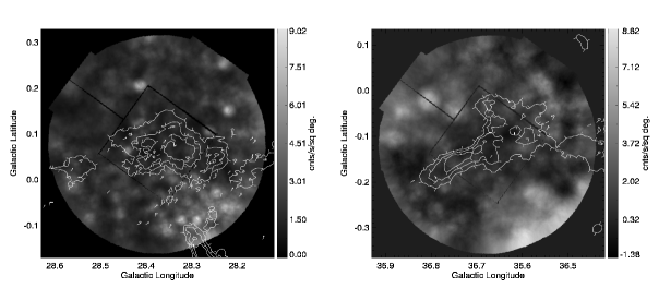
Figure 7: Smoothed XMM-Newton images in the energy range 0.35 keV to 1.25 keV of G28.37+0.07 (left panel) and G36.67$-$0.11(right panel). The contours are the same GRS contours shown in Figure 1. There is no obvious X-ray decrement at the location of the molecular clouds.

Table 1: Infrared Dark Cloud Properties

Name	l	b	D	Size	N(H2)
	deg.	deg.	kpc	sq. arcmin	$10^{22}$ cm-2
G28.37+0.07	28.37	+0.07	5.0	42	21
G36.67$-$0.11	36.67	$-$0.11	2.0	19	19

Table 2: Cloud Column Densities^†

Name	$N({\rm H})$			$N({\rm H}_{2})$			$N({\rm Total})$
	FG	BG		FG	BG		FG	BG
G28.37+0.07
On–cloud	0.5	1.0		0.4	2.1		1.3	5.2
Off–cloud	0.5	1.0		0.2	1.6		0.9	4.2
G36.67$-$0.11
On–cloud	0.5	1.0		0.1	1.4		0.7	3.8
Off–cloud	0.5	1.0		0.1	0.9		0.7	2.8

Table 3: Spectral Model Parameters

	G28.37+0.07						G36.67$-$0.11
	Column Fixed			Column Free			Column Fixed
Parameter	Value	Error		Value	Error		Value	Error
Column Density $\times 10^{22}$ cm-2
On–cloud, Foreground	1.3	$\cdots$		1.2	${}^{+0.003}_{-0.02}$		0.7	$\cdots$
On–cloud, Background	5.2	$\cdots$		3.9	${}^{0.6}_{-0.5}$		3.8	$\cdots$
Off–cloud, Foreground	0.9	$\cdots$		1.1	${}^{0.04}_{-0.03}$		0.7	$\cdots$
Off–cloud, Background	4.2	$\cdots$		2.9	${}^{0.3}_{-0.2}$		2.8	$\cdots$
LHB
kT(keV)	0.11	${}^{+3.7{\rm E}-3}_{-9.3{\rm E}-3}$		0.11	${}^{+8.3{\rm E}-3}_{-9.7{\rm E}-4}$		0.089	${}^{+4.7{\rm E}-3}_{-9.2{\rm E}-3}$
EM(cm-6 pc)	5.5E$-$4	${}^{+7.6{\rm E}-5}_{-7.0{\rm E}-5}$		5.4E$-$4	${}^{+6.0{\rm E}-5}_{-7.1{\rm E}-5}$		6.3E$-$4	${}^{+3.6{\rm E}-5}_{-6.8{\rm E}-5}$
Cool Foreground
kT(keV)	0.29	${}^{+1.5{\rm E}-2}_{-7.6{\rm E}-3}$		0.30	${}^{+2.8{\rm E}-2}_{-1.5{\rm}-2}$		$<0.35$	$\cdots$
EM(cm-6 pc)	4.6E$-$2	${}^{+6.9{\rm E}-3}_{-9.8{\rm E}-3}$		3.4E$-$2	${}^{+2.5{\rm E}-3}_{-1.0{\rm E}-2}$		$2.3{\rm E}-3$	${}^{+3.7{\rm E}-4}_{-1.5{\rm E}-3}$
Cool Background
kT(keV)	0.29	$\cdots$		0.30	$\cdots$		$<0.35$	$\cdots$
EM(cm-6 pc)	1.9E$-$3	${}^{+1.6{\rm E}-1}_{-1.9{\rm E}-3}$		0.00	${}^{+3.9{\rm E}-5}_{-0.0}$		5.8E$-$2	${}^{+1.9{\rm E}-2}_{-8.7{\rm E}-3}$
Galactic Ridge
kT(keV)	1.61	${}^{+0.25}_{-0.14}$		2.34	${}^{+0.35}_{-0.28}$		1.61	$\cdots$
EM(cm-6 pc)	2.2E$-$2	${}^{+1.5{\rm E}-3}_{-4.7{\rm E}-3}$		1.2E$-$2	${}^{+2.1{\rm E}-3}_{-1.1{\rm E}-3}$		8.2E$-$3	${}^{+1.6{\rm E}-3}_{-2.6{\rm E}-3}$
$\chi^{2}$	1373.5	$\cdots$		1348.1	$\cdots$		352.4	$\cdots$
dof	1236	$\cdots$		1231	$\cdots$		300	$\cdots$

References

- Almy et al. (2000) Almy, R. C., McCammon, D., Digel, S. W., Bronfman, L., & May, J. 2000, ApJ, 545, 290
- Anders & Grevesse (1989) Anders, E. & Grevesse, N. 1989, Geochim. Cosmochim. Acta, 53, 197
- Anderson & Bania (2009) Anderson, L. D. & Bania, T. M. 2009, ApJ, 690, 706
- Arnaud et al. (1996) Arnaud, K.A. in ASP Conf. Ser. 101, Astronomical Data Analysis Software and Systems V, ed. G. H. Jacoby & J. Barnes (San Francisco: ASP), 17
- Benjamin et al. (2003) Benjamin, R. A., et al. 2003, PASP, 115, 953
- Busfield et al. (2006) Busfield, A.L., Purcell, C.R., Hoare, M.G., Lumsden, S.L., Moore, T.J.T., Oudmaijer, R.D. 2006, MNRAS, 366, 1096
- Carey et al. (1998) Carey, Sean J., Clark, F. O., Egan, M. P., Price, S. D., Shipman, R. F., & Kuchar, T. A. 1998, ApJ, 508, 721
- Chen et al. (1997) Chen, L.-W., Fabian, A. C., & Gendreau, K. C. 1997, MNRAS, 285, 449
- Clemens (1985) Clemens, D. P. 1985, ApJ, 295, 422
- Dickey & Lockman (1990) Dickey, J. M., & Lockman, F. J. 1990, ARA&A, 28, 215
- Egan et al. (1998) Egan, M. P., Shipman, R. F., Price, S. D., Carey, S. J., Clark, F. O., & Cohen, M. 1998, ApJ, 494, 199
- Galeazzi et al. (2007) Galeazzi, M., Gupta, A., Covey, K., & Ursino, E. 2007, ApJ, 658, 1081
- Henley, Shelton, & Kuntz (2007) Henley, D. B., Shelton, R. L., & Kuntz, K. D. 2007, ApJ, 661, 304
- Henley & Shelton (2008) Henley, D. B. & Shelton, R. L. 2008, ApJ, 676, 335
- Jackson et al. (2002) Jackson, J. M., Bania, T. M., Simon, R., Kolpak, M., Clemens, D. P. & Heyer, M. 2002, ApJ, 566, 81
- Jackson et al. (2006) Jackson, J. M., Rathborne, J.M., Shah, R.Y., Simon, R., Bania, T.M., Clemens, D.P., Chambers, E.T., Johnson, A.M., Dormody, M. & Lavoie, R. 2006, ApJS, 163, 145
- Jackson et al. (2008) Jackson, J. M., Finn, S. C., Rathborne, J. M., Chambers, E. T., & Simon, R. 2008, ApJ, 680, 349
- Kalberla et al. (2005) Kalberla, P. M. W., Burton, W. B., Hartmann, D., Arnal, E. M., Bajaja, E., Morras, R., & Poppel, W. G. L. 2005, A&A, 440, 775
- Kolpak et al. (2003) Kolpak, M.A., Jackson, J.M., Bania, T.M., & Clemens, D.P. 2003, ApJ, 582, 756
- Kuchar & Bania (1993) Kuchar, T. A. & Bania, T. M. 1993, ApJ, 414, 664
- Kuntz & Snowden (2000) Kuntz, K. D., & Snowden, S. L. 2000, ApJ, 543, 195
- Kuntz & Snowden (2008) Kuntz, K. D., & Snowden, S. L. 2008, A&A, 478, 575
- Litzt, Burton & Bania (1981) Litzt, H. S., Burton, W. B., & Bania, T. M. 1981, ApJ, 246, 74
- Lumb et al. (2002) Lumb, D. H., Warwick, R. S., Page, M., & De Luca, A. 2002, A&A, 389, 93
- McCammon et al. (1983) McCammon, D., Burrows, D. N., Sanders, W. T., & Kraushaar, W. L. 1983, ApJ, 269, 107
- McCammon et al. (2002) McCammon, D., et al. 2002, ApJ, 576, 188
- Park et al. (1997) Park, S., Finley, J. P., Snowden, S. L., Dame, T. M. 1997, ApJ, 476, 77
- Roman-Duval et al. (2009) Roman-Duval, J., Jackson, J. M., Heyer, M., Johnson, A., Rathborne, J., Shah, R., & Simon, R. 2009, ApJ, 699, 1153
- Simon et al. (2001) Simon, R., Jackson, J.M., Clemens, D.P., & Bania, T.M. 2001, ApJ, 551, 747
- Simon et al. (2006) Simon, R., Rathborne, J. M., Shah, R. Y., Jackson, J. M., & Chambers, E. T. 2006, ApJ, 653, 1325
- Smith & Cox (2001) Smith, R. K. & Cox, D. P. 2001, ApJS, 134, 283
- Smith et al. (2001) Smith, R. K., Brickhouse, N. S., Liedahl, D. A., & Raymond, J. C. 2001, ApJ, 556, L91
- Smith et al. (2005) Smith, R. K., Edgar, R. J., Plucinsky, P. P., Wargelin, B. J., Freeman, P. E., & Biller, B. A. 2005, ApJ, 623, 225
- Smith et al. (2007) Smith, R. K. et al. 2007, PASP, 59, 141
- Snowden et al. (1990) Snowden, S. L., Cox, D. P., McCammon, D., & Sanders, W. T. 1990, ApJ, 354, 211
- Snowden, McCammon, & Verter (1993) Snowden, S. L.; McCammon, D.; & Verter, F. 1993, ApJ, 409, 21
- Snowden et al. (1994) Snowden, S. L.; McCammon, D.; Burrows, D. N.; Mendenhall, J. A. 1994, ApJ, 424,714
- Snowden et al. (1997) Snowden, S. L., Egger, R., Freyberg, M. J., McCammon, D., Plucinsky, P. P., Sanders, W. T., Schmitt, J. H. M. M., Truemper, J., & Voges, W. 1997, ApJ, 485, 125
- Snowden et al. (1998) Snowden, S. L., Egger, R., Finkbeiner, D. P., Freyberg, M. J., & Plucinsky, P. P. 1998, ApJ, 493, 715
- Snowden et al. (2000) Snowden, S. L., Freyberg, M. J., Kuntz, K. D., & Sanders, W. T. 2000, 128, 171
- Snowden, Collier & Kuntz (2004) Snowden, S. L., Collier, M. R., & Kuntz, K. D. 2004, ApJ, 610, 1182
- Snowden et al. (2008) Snowden, S. L., Mushotzky, R. M., Kuntz, K. D., & Davis, D. S. 2008, A&A, 478, 615
- Stil et al. (2006) Stil, J. M., et al. 2006, AJ, 132, 1158
- Williams & Maddalena (1996) Williams, J. P. & Maddalena, R. J. 1996, ApJ, 464, 247