Localization in one dimensional lattices with non-nearest-neighbor hopping: Generalized Anderson and Aubry-André models

Abstract

We study the quantum localization phenomena of noninteracting particles in one-dimensional lattices based on tight-binding models with various forms of hopping terms beyond the nearest neighbor, which are generalizations of the famous Aubry-André and noninteracting Anderson model. For the case with deterministic disordered potential induced by a secondary incommensurate lattice (i.e. the Aubry-André model), we identify a class of self-dual models, for which the boundary between localized and extended eigenstates are determined analytically by employing a generalized Aubry-André transformation. We also numerically investigate the localization properties of nondual models with next-nearest-neighbor hopping, Gaussian, and power-law decay hopping terms. We find that even for these non-dual models, the numerically obtained mobility edges can be well approximated by the analytically obtained condition for localization transition in the self dual models, as long as the decay of the hopping rate with respect to distance is sufficiently fast. For the disordered potential with genuinely random character, we examine scenarios with next-nearest-neighbor hopping, exponential, Gaussian, and power-law decay hopping terms numerically. We find that the higher-order hopping terms can remove the symmetry in the localization length about the energy band center compared to the Anderson model. Furthermore, our results demonstrate that for the power-law decay case, there exists a critical exponent below which mobility edges can be found. Our theoretical results could, in principle, be directly tested in shallow atomic optical lattice systems enabling non-nearest-neighbor hopping.

I Introduction

Quantum transport of matter waves in the presence of disorder has long been a topic of interest for condensed-matter physicists. For one-dimensional (1D) noninteracting systems, one of the oldest and most extensively studied models for quantum transport is the single-band, nearest-neighbor (nn) tight-binding model,

$$t_{1}(u_{n+1}+u_{n-1})+V_{n}u_{n}=Eu_{n},$$ (1)

where $t_{1}$ is the nn hopping integral term and $V_{n}$ is the on-site disordered potential Kramer and MacKinnon (1993). One of the main merits of Eq. (1) is its simple form, which lends itself to fast numerical analysis, as well as exact theoretical statements on quantum transport in some cases. Arguably the most well known of the latter is when $V_{n}$ is bounded, uncorrelated disorder (i.e., the noninteracting Anderson model Anderson (1958)), where it can be shown that all eigenstates of the system are localized for any nonzero potential strength. Another well-known example is the 1D incommensurate problem [in particular, $V_{n}=V\cos(2\pi\alpha n+\delta)$, where $\alpha$ is irrational] studied by Aubry and André where all eigenstates of the system are extended for potential strength below a threshold value ($V_{c}=2t_{1}$) and localized above this threshold Aubry and André (1980). Conversely, this simple form given by Eq. (1) makes it difficult to study directly in solid-state systems, where the disorder is difficult to control reliably and interactions can rarely be ignored. However, recent advances in the manipulation of ultracold atoms in optical lattices provide a powerful tool for directly examining quantum transport in fundamental models such as Eq. (1). This has been most notably demonstrated in recent experiments conducted by Billy $et$ $al.$, where Anderson localization was directly observed in a Bose-Einstein condensate (BEC) subjected to a random laser speckle potential Billy et al. (2008), and similarly in experiments conducted by Roati $et$ $al.$, where Aubry-André duality was directly observed in a BEC loaded into a quasi-periodic optical lattice Roati et al. (2008); *Modugno2009. These feats, which previously eluded experimental observation for decades, illustrate the potential of ultracold atomic systems to experimentally probe fundamental quantum phenomena. Considering the degree of control afforded in ultracold atomic systems, we can systematically relax, in a controlled manner, basic assumptions inherent in Eq. (1) and directly study their influence on quantum transport and how it differs from the well-known Anderson and Aubry-André results. It is this potential in ultracold atomic systems that motivates our present work, where we examine quantum transport in tight-binding, non-interacting models that are extensions of Eq. (1). In particular, we relax the nn tight-binding assumption and theoretically examine transport in models with long and short-range hopping schemes. Such models should be representative of diffuse gases of ultracold atoms loaded into fairly shallow optical lattices.

We can go beyond the nn coupling assumption while still remaining in the tight-binding framework by including higher-order hopping terms. The general form of such a model with on-site disorder is given by

$$\sum_{m}t_{m}u_{n+m}+V_{n}u_{n}=Eu_{n},$$ (2)

where the tight-biding terms $t_{m}$ may assume a variety of forms. There is a small, but growing body of numerical and analytical work examining transport in the context of this generalized model Biddle et al. (2009); Boers et al. (2007); Riklund et al. (1986); de Moura et al. (2005); Malyshev et al. (2004); Xiong and Zhang (2003); Rodríguez et al. (2003); Das Sarma et al. (1986). In an effort to extend this growing body of work, we wish to investigate transport through various forms of Eq. (2) with both incommensurate and random on-site potentials. In particular, we study transport in tight-binding models with next-nearest-neighbor (nnn) hopping (the $t_{1}-t_{2}$ model) and models incorporating an infinite number of hopping terms that decay by an exponential, Gaussian, or inverse power law. Since we examine both deterministic bichromatic potentials and random potentials, this report is divided into two sections. The first section examines the case of incommensurate potentials by first studying the exponential hopping model, which has been shown to have an analytical mobility edgeBiddle and Das Sarma (2010), then approximately extrapolating these results to predict the mobility edges in the nnn, Gaussian, and inverse-power-law hopping models [Mobilityedgesortheexistenceofextendedstatesindisordered1Dsystemsarenotuniquetotight-bindingmodelswithhigherorderhoppingterms.See; forexample; ]Soukoulis82; *DasSarma88; *XieDasSarma88; *Scarola06. The second section numerically examines Eq. (2) with nnn, exponential, Gaussian, and inverse-power-law hopping for randomly disordered potentials and highlights how localization in these models is markedly different compared to what is seen in the case of the nn Anderson model.

II Incommensurate Potentials

II.1 Self Dual models

One of the first models to examine quantum transport in 1D incommensurate potentials is the so-called Aubry-André (AA) modelAubry and André (1980). In this model, the on-site term in Eq. (1) is a cosine with frequency incommensurate with the primary lattice: $V_{n}=V\cos(2\pi\alpha n+\delta)$ where $\alpha$ is an irrational number and $\delta$ is an arbitrary phase. It has been shown that this model is self-dual under the transformation,

$$u_{n}=\sum_{m}f_{m}e^{im(2\pi\alpha n+\delta)}e^{i\beta n},$$ (3)

when $V=2t_{1}$ (i.e. $f_{m}$ satisfies the same eigenvalue equation as $u_{n}$). Also, under Eq. (3), if the eigenstate $u_{n}$ is spatially localized, then the eigenstate of the dual problem, $f_{m}$, is spatially extended and vice versa. Using this property and the Thouless formula for incommensurate potentials Thouless (1972), it is argued that all eigenstates are localized for $V>2t_{1}$ and extended for $V<2t_{1}$. The case where $V=2t_{1}$ is especially interesting and has been shown to yield a singular continuous eigenspectrum, which forms a Cantor set in the thermodynamic limit Bellissard and Simon (1982). Furthermore AA duality can be shown to have a more general form Sokoloff (1985). Consider the model,

$$\sum_{m}t_{m}u_{n+m}+V_{0}v_{n}u_{n}=Eu_{n}.$$ (4)

If the on-site potential and the hopping terms satisfy the relation,

$$v_{n}=\sum_{m}t_{m}e^{im(2\pi\alpha n+\delta)},$$ (5)

then this model also possesses an AA-like duality.

Other models have been shown to possess self-duality similar to the AA model Das Sarma et al. (1986); Biddle and Das Sarma (2010). The particular model we consider here, given by

$$Eu_{n}=\sum_{n^{\prime}\neq n}te^{-p|n-n^{\prime}|}u_{n^{\prime}}+V\cos(2\pi\alpha n+\delta)u_{n},$$ (6)

is especially interesting because its self-duality condition naturally predicts energy-dependent mobility edges, in contrast to the AA modelBiddle and Das Sarma (2010). To see this we now reiterate the results given in the previous work on this model to show that Eq. (6) does have a self-dual condition and we expand on the previous work to show that this self-dual condition does indeed define a mobility edge.

We begin by defining the parameter, $p_{0}>0$ such that

$$(E+t)-V\cos(2\pi\alpha n+\delta)=\Omega T_{n},$$ (7)

$$T_{n}=\frac{\cosh(p_{0})-\cos(2\pi\alpha n+\delta)}{\sinh(p_{0})},$$ (8)

$$\Omega=\sqrt{(E+t)^{2}-V^{2}}.$$ (9)

Then it follows that $(E+t)/V=\cosh(p_{0})$ and we can rewrite Eq. (6) as

$$\Omega T_{n}u_{n}=\sum_{n^{\prime}}te^{-p|n-n^{\prime}|}u_{n^{\prime}}.$$ (10)

If we now consider the transformation

$$\tilde{u}_{m}=\sum_{n}e^{im(2\pi\alpha n+\delta)}T_{n}u_{n},$$ (11)

and note that for $p>0$ we have the identity

$$T_{n}^{-1}=\sum_{m}e^{-p|m|}e^{im(2\pi\alpha n+\delta)},$$ (12)

then it follows that the state $\tilde{u}_{m}$ satisfies the equation

$$\Omega\tilde{T}_{m}\tilde{u}_{m}=\sum_{m^{\prime}}te^{-p_{0}|m-m^{\prime}|}\tilde{u}_{m^{\prime}},$$ (13)

where $\tilde{T}_{m}$ is given by

$$\tilde{T}_{m}=\frac{\cosh(p)-\cos(2\pi\alpha m+\delta)}{\sinh(p)}.$$ (14)

We see that Eq. (10) is self-dual under the transformation Eq. (11) when $p=p_{0}$, or equivalently $\cosh(p)=\cosh(p_{0})$ for $p,p_{0}>0$. Thus, the duality condition for Eq. (6) is given by

$$\cosh(p)=\frac{E+t}{V}.$$ (15)

Since the transformation given by Eq. (11) transforms localized states to extended states and vice versa [similar to Eq. (3)], we expect that the eigenstates of the system are critical (neither localized nor extended) when Eq. (15) is satisfied.

Similar to the arguments made by Aubry and André for the AA model, we now expand on the conjecture made in the previous workBiddle and Das Sarma (2010) and argue that the eigenstates of Eq. (10) are localized for $p>p_{0}$ and extended for $p<p_{0}$ [i.e. that Eq. (15) does, indeed, define a mobility edge]. Since the Thouless formula used by Aubry and André was derived for models of the form of Eq. (1), we can not use it for our particular model. Therefore, our first step is to generalize the idea of the Thouless formula for the long-range hopping model. To do so, we treat $\Omega$ as the eigenvalue and consider the Green’s matrix,

$$G(\Omega)_{m,n}=(\Omega\overline{\mathrm{I}}-\overline{\mathrm{H}})_{m,n}^{-1}$$ (16)

$$=\frac{\mathrm{cofactor}(\Omega\overline{\mathrm{I}}-\overline{\mathrm{H}})_{m,n}}{\prod_{\beta}(\Omega-\Omega_{\beta})},$$ (17)

where the cofactor is the appropriately signed determinant with the $m$th row and $n$th column removed and $\overline{\mathrm{H}}$ is the Hamiltonian corresponding to the eigenvalue equation given in Eq. (10) where we have set $t=1$ without loss of generality; $\overline{\mathrm{I}}$ is the identity matrix. Assuming a nondegenerate eigenspectrum, the Green’s matrix has a simple pole for each eigenvalue, $\Omega_{\mu}$. Since, by definition, the residue of $G(\Omega^{(\mu)})_{m,n}$ is the product of the $m$th and $n$th elements of the eigenvector (i.e. $Res(G(\Omega)_{m,n},\Omega_{\mu})=u_{m}^{(\mu)}u_{n}^{(\mu)}$)Thouless (1972), we have for the product of the first and last elements of the eigenvector

$$u_{1}^{(\mu)}u_{N}^{(\mu)}=\frac{\mathrm{cofactor}(\Omega_{\mu}\overline{\mathrm{I}}-\overline{\mathrm{H}})_{1,N}}{\prod_{\beta\neq\mu}(\Omega_{\mu}-\Omega_{\beta})}.$$ (18)

If the state is exponentially localized about the site $n^{\prime}$, then we expect $u_{n}\sim\exp(-\gamma|n^{\prime}-n|)$, where $\gamma\geq 0$ is the characteristic (or Lyapunov) exponent. Therefore the product $u_{1}u_{N}\sim\exp(-\gamma(N-1))$. Thus, the characteristic exponent for large $N$ is given by

$$\gamma(\Omega_{\mu}) = \lim_{N\to\infty}-(N-1)^{-1}\ln|u_{1}^{(\mu)}u_{N}^{(\mu)}|$$ (19)

$$= \lim_{N\to\infty}(N-1)^{-1}(\sum_{\beta\neq\mu}\ln|\Omega_{\mu}-\Omega_{\beta}|$$

$$- \ln|\mathrm{cofactor}(\Omega_{\mu}\overline{\mathrm{I}}-\overline{\mathrm{H}})_{1,N}|).$$

This is the generalized Thouless relation for the characteristic exponent of a wavefunction. For the case where $\overline{\mathrm{H}}$ is given by Eq. (10), the cofactor takes on the form:

$$\mathrm{cofactor}(\Omega_{\mu}\overline{\mathrm{I}}-\overline{\mathrm{H}})_{1,N}=\Omega_{\mu}^{N-2}e^{-(N-1)p}T_{N}^{-1}.$$ (20)

Then we have for the characteristic exponent,

$$\gamma(\Omega_{\mu})=p-\ln|\Omega_{\mu}|+\lim_{N\to\infty}(N-1)^{-1}\sum_{\beta\neq\mu}\ln|\Omega_{\mu}-\Omega_{\beta}|.$$ (21)

We now compare the characteristic exponents of the eigenvectors of Eq. (10), which we denote as $\gamma(\Omega)$, with the exponents of the dual problem Eq. (13), denoted as $\tilde{\gamma}(\Omega)$. Since the eigenvalue $\Omega$ is not changed by the transformation given by Eq. (11), we expect the summation term on the right-hand side of Eq. (21) to be equal for both Eq. (10) and Eq. (13). Therefore, the characteristic exponents have the following relation:

$$\gamma(\Omega)=\tilde{\gamma}(\Omega)+(p-p_{0}).$$ (22)

Considering the case when $p>p_{0}$, since $\tilde{\gamma}(\Omega)\geq 0$, it follows that $\gamma(\Omega)>0$ and therefore the eigenstate, $u_{n}$ is localized while the dual state, $\tilde{u}_{n}$ is extended. Similarly, when $p_{0}>p$, we can argue that $\tilde{\gamma}(\Omega)>0$ and therefore the dual state, $\tilde{u}_{n}$, is localized while $u_{n}$ is extended. Therefore, returning to the original problem given by Eq. (6) and using the fact that $\cosh(p_{0})$ is a monotonically increasing function of $p_{0}>0$, it follows that the eigenstates are localized for $(E+t)/V<\cosh(p)$ and extended for $(E+t)/V>\cosh(p)$.

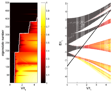
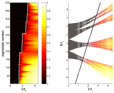
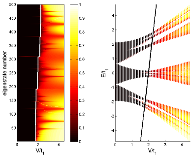
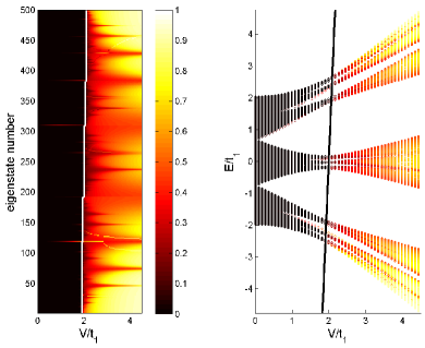
Figure 1: Energy eigenvalues and inverse participation ratios of Eq. (6) with 500 lattice sites and $\alpha=(\sqrt{5}-1)/2$ for 1 $p=1$, 1 $p=2$, 1 $p=3$, 1 $p=4$. The solid line represents the analytical boundary between spatially localized and spatially extended states.

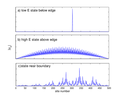
Figure 2: Eigenstates of Eq. (6) with 500 lattice sites, $\alpha=(\sqrt{5}-1)/2$, $V=1.8$, and $p=1.5$ for different energy eigenvalues: a) low energy localized state below the mobility edge b) high energy extended state above the mobility edge c) critical state near the mobility edge.

Similar to the AA model, the self-duality described above has a general form, considering, again, a model of the form given in Eq. (4). The model will have this form of self-duality if the on-site potential and the hopping terms satisfy the relation:

$$\frac{A}{B-v_{n}}=\sum_{m}t_{m}e^{im(2\pi\alpha n+\delta)}$$ (23)

where $A$ and $B$ are constants. In particular, the constant $B$ gives the slope of the the duality condition (i.e., $B=E/V_{0}$).

We now numerically examine localization in Eq. (6) [and equivalently Eq. (10)] by calculating the inverse participation ratio (IPR) of the wave functions, given by:

$$\text{IPR}^{(i)}=\frac{\sum_{n}|u^{(i)}_{n}|^{4}}{({\sum_{n}|u^{(i)}_{n}|^{2}})^{2}},$$ (24)

where the superscript $i$ denote the $i$ eigenstate. The IPR approaches zero for spatially extended wave functions and is finite for localized wave functions, and hence has a useful diagnostic role. Fig. 1 plots energy eigenvalues (or eigenstate number) and the IPR of the corresponding wave functions for Eq. (6) as a function of potential strength, $V$, with $\alpha=(\sqrt{5}-1)/2$ and $p=1$, 2, 3, or 4. The solid curves in the figures represent the boundary given in Eq. (15). From the figure we see that IPR values are approximately zero for energies above the boundary and are finite for energies below the boundary. This supports our assertion that the mobility edge is, indeed, given by Eq. (15).

In Fig. 2, we directly examine sample eigenstates in each regime (i.e., localized, extended, and near the mobility edge) for $p=1.5$ and $V=1.8$. We see that the wavefunction is localized for low energies [Fig 2a], extended for high energies [Fig 2b], and critical near the boundary [Fig 2c].

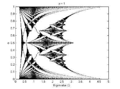
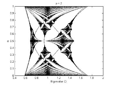
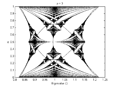
Figure 3: Eigenspectrum of Eq. (10) with varying $\alpha$ for 3 $p=1$ , 3 $p=2$, and 3 $p=3$.

Finally, we examine the eigenvalues of Eq. (10) for different values of $\alpha$ at the duality point ($p=p_{0}$) where we expect the eigenspectrum to form a fractal set for large $N$. The results of this are given in Fig. 3. In the figure, we see that for large values of $p$, the eigenspectrum closely resembles the well-known Hofstadter’s butterfly which results from the solutions of Harper’s equation Harper (1955); Hofstadter (1976). For smaller values of $p$, however, we see a generalized form of Hofstadter’s butterfly that is not symmetrical about the the band center, but skewed toward lower eigenvalues. The self-similarity in the figure suggests that the eigenspectrum does, indeed, form a Cantor set at the duality point in the thermodynamic limit.

II.2 Nondual models

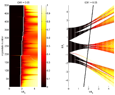
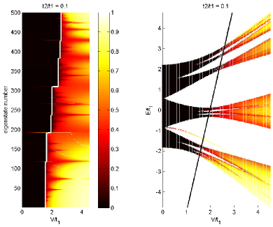
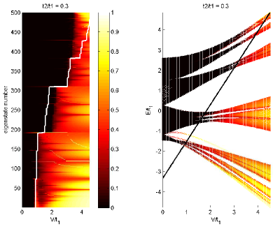
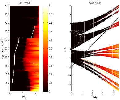
Figure 4: Inverse participation ratios and energy eigenvalues of all eigenstates of Eq. (25) with 500 lattice sites and $\alpha=(\sqrt{5}-1)/2$ for $t_{2}/t_{1}=$ 4 0.05, 4 0.1, 4 0.3, 4 0.5. The solid curves represent the approximate boundary between spatially localized and spatially extended states.

General realizations of Eq. (2) with an incommensurate potential should not be expected to satisfy either Eq. (5) or Eq. (23). Thus, the mobility edges in non-dual incommensurate problems may not be discernible by theoretical means. However, approximate theoretical statements can be made for some non-dual models with hopping terms that fall off in some general manner. If this fall off is fast enough, then the localization transitions in these models are largely determined by the ratio $t_{2}/t_{1}$. This ratio can be used to determine an approximately equivalent model of the form of Eq. (6), which, as shown in the above section, has an exact theoretical localization boundary. To show this possibility, we numerically examine the eigenstates of several non-dual models. In particular, we examine the $t_{1}-t_{2}$ model, the Gaussian hopping model, and the inverse-power-law hopping model with an incommensurate potential and see how closely the approximate localization boundary matches with the numerically observed one.

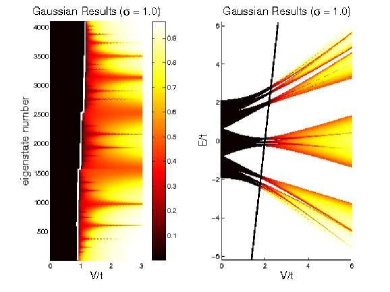
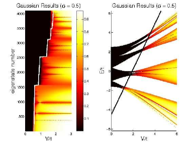
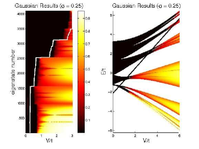
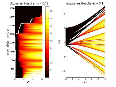
Figure 5: Inverse participation ratios and energy eigenvalues of all eigenstates of Eq. (26) with 4096 lattice sites and $\alpha=(\sqrt{5}-1)/2$ for $\sigma=$ (a) 1.0, (b) 0.5, (c) 0.25, and (d) 0.10. The solid curves represent the approximate boundary between spatially localized and spatially extended states.

The $t_{1}-t_{2}$ model is the nnn extension of the AA model and is given by

$$\left(\begin{array}[]{c}t_{2}(u_{n+2}+u_{n-2})+t_{1}(u_{n+1}+u_{n-1})\\ +V\cos(2\pi\alpha n+\delta)u_{n}\end{array}\right)=Eu_{n}.$$ (25)

The parameters of the approximately equivalent exponential hopping model [Eq. (6)] are given by $p=\ln(t_{1}/t_{2})$ and $t=t_{1}e^{p}$. Using Eq. (15), we can approximate the boundary between localized and extended states. To examine this approximation we calculate the IPR of the eigenstates of Eq. (25). The results are given in Fig. 4 for 500 lattice sites, $\alpha=(\sqrt{5}-1)/2$ and various values of the ratio $t_{2}/t_{1}$. The solid lines in the figure give the approximate mobility edge given by Eq. (15). From the figure, we see that for small values of $t_{2}/t_{1}$, the approximate boundary is in good qualitative agreement with the numerical IPR results. For larger values ($t_{2}/t_{1}\gtrsim 0.3$), however the boundary differs considerably from the linear condition in Eq. (15).

The tight-binding incommensurate model with Gaussian hopping has the form:

$$\sum_{n^{\prime}\neq n}e^{-\sigma|n-n^{\prime}|^{2}}u_{n^{\prime}}+V\cos(2\pi\alpha n+\delta)u_{n}=Eu_{n}.$$ (26)

Similar to the $t_{1}-t_{2}$ model, the approximately equivalent exponential hopping model can be determined from the ratio $t_{2}/t_{1}$, which yields $p=3\sigma$. The IPR results for this model are given in Fig. 5 [again, $\alpha=(\sqrt{5}-1)/2$]. In this figure, we see that the approximate boundary is in good qualitative agreement with the numerical results for larger values of $\sigma$. Small values of $\sigma$, however, result in very interesting energy-dependent mobility edges that are not linear in potential strength, which is similar to the $t_{1}-t_{2}$ results for large values of $t_{1}/t_{2}$.

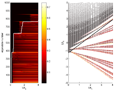
(a) $r=1/3$

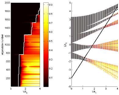
(b) $r=2$

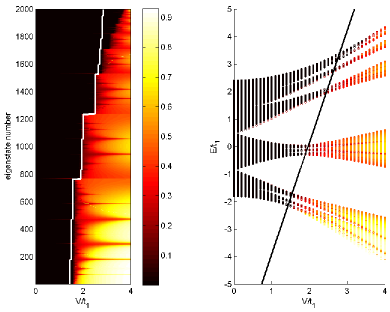
(c) $r=3$

Figure 6: Inverse participation ratios and energy eigenvalues of all eigenstates of Eq. (27) with 2000 lattice sites and $\alpha=(\sqrt{5}-1)/2$ for various values of $r$. The solid curves represent the approximate boundary between spatially localized and spatially extended states.

For power law decay in the hopping terms, we examine the model:

$$\sum_{n^{\prime}\neq n}\frac{u_{n^{\prime}}}{|n-n^{\prime}|^{r}}+V\cos(2\pi\alpha n+\delta)=Eu_{n}.$$ (27)

In this case, the exponential coefficient, $p$ is given by $p=r\ln(2)$. Fig 6 gives IPR results for this model with $\alpha=(\sqrt{5}-1)/2$ and $r=1/3$ [Fig 6(a)], $r=2$ [Fig 6(b)], and $r=3$ [Fig 6(c)]. In each of these cases, the approximate localization boundary is in good qualitative agreement with the numerical results.

From the above numerical results, we see that the localization boundary for the exponential hopping model gives a good qualitative agreement for the Gaussian and inverse-power-law hopping models with large-enough decay coefficients (i.e., $r$ and $\sigma\gtrsim 1$). Thus, we believe that the localization boundary for any tight-binding model with hopping terms that decay fast enough can be approximated by the results of the exponential hopping model. In general, however, we see that the energy-dependent mobility edges in the non-dual models are not linear in $V$ as with the case in the exponential hopping model. Whether there is an exact theoretical statement to describe these peculiar mobility edges is still an open question.

III Random disorder

We examine the case of a random potential in the tight binding framework in the context of both the nnn model (i.e. the $t_{1}-t_{2}$ model) and extended schemes where the coupling may be short ranged in the sense of decaying exponentially (or more rapidly, as in a Gaussian decay) or long-ranged with a power law decay.

We examine the effects of a random potential directly in the context of characteristics of the eigenstates, by studying the IPR, which provides information as to the extent of localization. We calculate the IPR versus eigenstate number for a range of random potential strengths, which will tend to localize states.

We produce surface graphs of the IPR to show the characteristics of the eigenstates with respect to localization. In addition, one may calculate histograms of the IPR instead of preparing surface plots with respect to eigenstate number and the width of the potential. The former complement the latter by showing how the statistical weight for a particular IPR value evolves with increasing system size.

We find in both the surface plots and in the histograms a convergence toward bulk behavior, where self-averaging in sufficiently large systems reduces the differences in the characteristics of the eigenstates corresponding to independently generated random potential realizations. In the thermodynamic limit, the type of tight-binding coupling scheme and the overall statistical characteristics of the random potential are the factors which determine the distribution of the properties of the eigenstates.

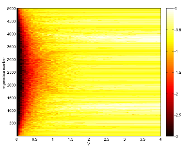
(a) $t_{2}=0$

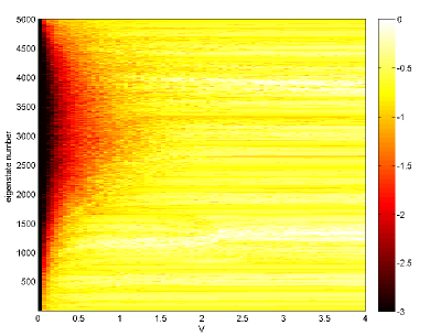
(b) $t_{2}=0.2$

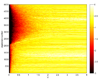
(c) $t_{2}=0.4$

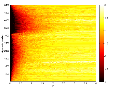
(d) $t_{2}=0.8$

Figure 7: (Color online) Suface plot of the base 10 logarithm of the IPRs for the $t_{1}-t_{2}$ model with a random, binary potential for 5000 lattice sites.

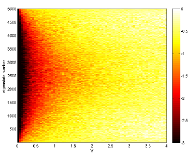
(a) $t_{2}=0$

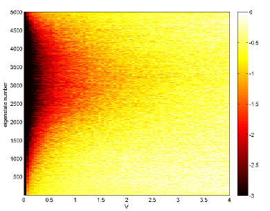
(b) $t_{2}=0.2$

Figure 8: (Color online) Surface plots of the base 10 logarithm of the IPRs for the $t_{1}-t_{2}$ model with a random, uniformly distributed potential for 5000 lattice sites.

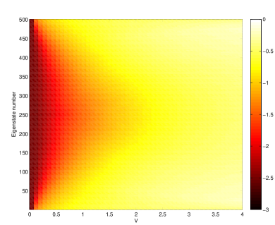
(a) $t_{2}=0$

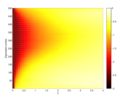
(b) $t_{2}=0.2$

Figure 9: (Color online) Surface plots of the base 10 logarithm of the IPRs for the $t_{1}-t_{2}$ model averaged over 100 realizations of random, uniformly distributed potentials with 500 lattice sites.

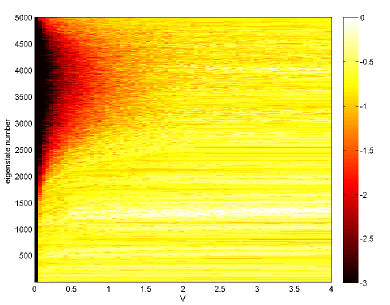
(a) $\sigma=0.25$

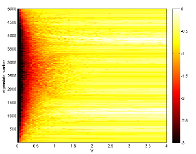
(b) $\sigma=1$

Figure 10: (Color online) Surface plots of the base 10 logarithm of the IPRs for the Gaussian hopping model with a random, binary potential for 5000 lattice sites.

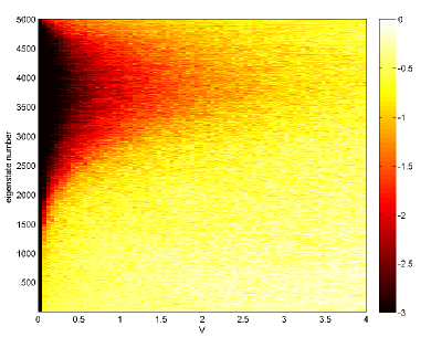
(a) $\sigma=0.25$

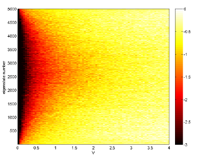
(b) $\sigma=1$

Figure 11: (Color online) Surface plots of the base 10 logarithm of the IPRs for the Gaussian hopping model with a random, uniformly distributed potential for 5000 lattice sites.

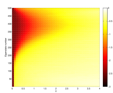
(a) $\sigma=0.25$

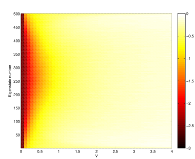
(b) $\sigma=1$

Figure 12: (Color online) Surface plots of the base 10 logarithm of the IPRs for the Gaussian hopping model averaged over 100 realizations of random, uniformly distributed potentials with 500 lattice sites.

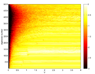
(a) $p=1$

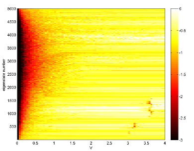
(b) $p=2$

Figure 13: (Color online) Surface plots of the base 10 logarithm of the IPRs for the exponential hopping model with a random, binary potential for 5000 lattice sites.

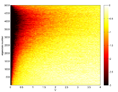
(a) $p=1$

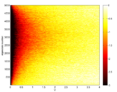
(b) $p=2$

Figure 14: (Color online) Surface plots of the base 10 logarithm of the IPRs for the exponential hopping model with a random, uniformly distributed potential for 5000 lattice sites.

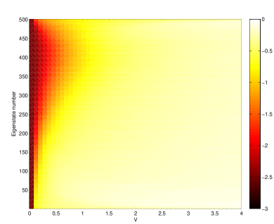
(a) $p=1$

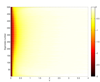
(b) $p=2$

Figure 15: (Color online) Surface plots of the base 10 logarithm of the IPRs for the exponential hopping model averaged over 100 realizations of random, uniformly distributed potentials with 500 lattice sites.

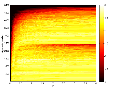
(a) $r=1/3$

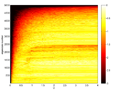
(b) $r=1$

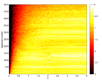
(c) $r=2$

Figure 16: (Color online) Surface plots of the base 10 logarithm of the IPRs for the inverse-power-law model with a random, binary potential for 5000 lattice sites.

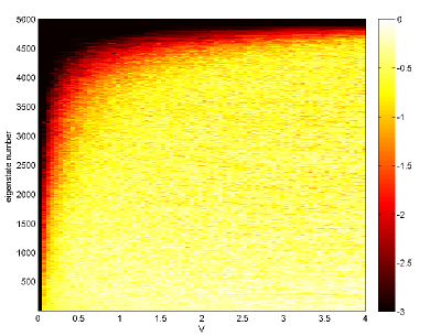
(a) $r=1/3$

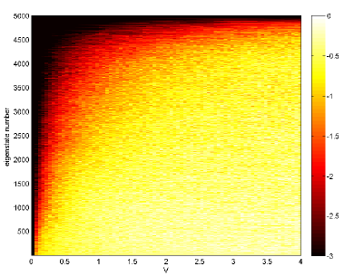
(b) $r=1$

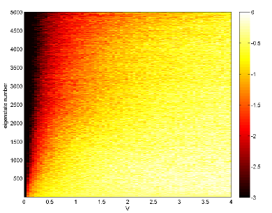
(c) $r=2$

Figure 17: (Color online) Surface plots of the base 10 logarithm of the IPRs for the inverse-power-law model with a random, uniformly distributed potential for 5000 lattice sites.

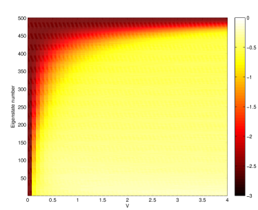
(a) $r=1/3$

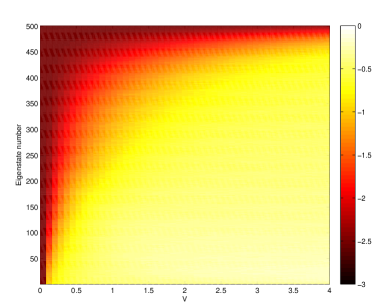
(b) $r=1$

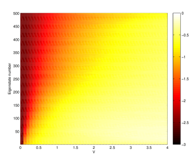
(c) $r=2$

Figure 18: (Color online) Surface plots of the base 10 logarithm of the IPRs for the inverse-power-law model averaged over 100 realizations of random, uniformly distributed potentials with 500 lattice sites.

In implementing the on-site random potential, we operate either in terms of a binary potential where the potential at a particular site assumes the value $V$ or $-V$ with equal probability or a continuous one which is chosen with uniform probability between the bounds $V$ and $-V$. In either case, the strength of the random potential may be considered to be parameterized by $V$. We begin by studying the $t_{1}-t_{2}$ model with random on-site disorder. Fig. 7 gives the IPR as a function of the disorder strength, $V$, and the eigenstate number, $i$, for the eigenstates of the $t_{1}-t_{2}$ tight-binding model with a binary random on-site potential and 5000 lattice sites. In the figure we see that for $t_{2}=0$, we have the 1D Anderson model where localization is relatively weak at the band center and comparatively strong near the band edges Kramer and MacKinnon (1993). However as we increase $t_{2}$, we see that the weakly localized states shift to higher energies toward the top band edge. Moreover, as the relative value of $t_{2}$ is increased, cross sections of the IPR along the eigenstate number axis develop a bimodal profile. In the case where $t_{2}=0.8$ [Fig. 7(d)] the bimodal structure is particularly stark. In this case we begin to see two distinct regions of weakly localized states, in contrast to the Anderson case where the localization is weakest in the band center, giving way to more strongly localized states at the band edges. We also obtain qualitatively similar results when we consider a uniformly distributed, rather than binary, random potential (Fig. 8).

In addition to surface plots produced for a single realization of the random potential, we also generate surface plots of the IPR with respect to $V$ and eigenstate number where the results are averaged over a large number of random configurations. In particular, in Fig. 9, we average the IPR over 100 different realizations of an on-site, uniformly distributed random potential for the $t_{1}-t_{2}$ model with 500 lattice sites. The qualitative similarities among Figures 7, 8, and 9 suggest that the localization behavior is self-averaging in the sense that statistical fluctuations play a small role in determining the characteristics of the system if the system size $N$ is sufficiently large.

We now study the randomly disordered tight-binding model with a Gaussian decay in the hopping terms. Fig. 10 and Fig. 11 give the IPR as a function of potential strength, $V$, and eigenstate number, $i$, of the eigenstates of the Gaussian decay tight-binding model [i.e. $t_{m}=\exp(-\sigma|m|^{2})$] with a random binary and random uniform on-site potential, respectively, and 5000 lattice sites. In both Fig. 10 and Fig. 11, we see that for small $\sigma$, the weakly localized states appear at higher energies in comparison to the Anderson model (similar to the $t_{1}-t_{2}$ model for large $t_{2}$). For larger $\sigma$, the IPR is qualitatively similar to that of the Anderson model case as would be expected given the very rapid decay which strongly suppresses hopping beyond the nearest neighbors for which the Anderson model is an idealization with hopping confined strictly to nearest neighbors. We also average the IPR over 100 different realizations of an on-site, uniformly distributed random potential for the Gaussian decay hopping model with 500 lattice sites and report the results in Fig. 12. Again, the qualitative similarities among Fig. 10, Fig. 11, and Fig. 12 suggest that self-averaging is at work in the localization characteristics of the eigenstates. The averaging over many realizations of disorder has the effect of removing much of the graininess due to statistical fluctuations which would not appear in the bulk limit and seem to be finite size artifacts, while preserving more smoothly varying characteristics which appear to be associated with the bulk limit.

Similar results can be seen in the randomly disordered tight-binding model with exponentially decaying hopping terms. Figures 13 and 14 give the IPR as a function of potential strength, $V$, and eigenstate number, $i$, of the eigenstates of the exponential hopping tight-binding model [i.e. $t_{m}=\exp(-p|m|)$] with a random, binary and random, uniform on-site potential, respectively, and 5000 lattice sites. Similar to the Gaussian decay model, we see that for small $p$, the weakly localized states appear at higher energies compared to the Anderson case, and for larger $p$, the IPR approaches that in the Anderson case. Moreover, just as we saw in the $t_{1}-t_{2}$ and Gaussian models, evidence of self-averaging may be seen by examining the average of the IPR over 100 realizations of a uniform random potential with 500 lattice sites (Fig. 15).

We now turn to the randomly disordered tight-binding extended model with hopping terms that decay by an inverse-power-law. Since this slow form of decay essentially allows for long-range hopping, the localization characteristics of this model differ more from those of the Anderson model, where the hopping scheme is short-ranged, than those of the other models we have investigated. In Figures 16 and 17, we show the IPR for a random, binary and random, uniform on-site potential respectively as a function of potential strength, $V$, and eigenstate number, $i$, of the eigenstates of the tight-binding model with hopping terms that fall off as $t_{m}=1/|m|^{r}$. In these figures, we see that the states near the top band edge are weakly localized, and the top band edge is possibly de-localized for $r=1/3$ and $r=1$. This supports earlier theoretical and numerical work which suggests that there is, indeed, a mobility edge at the top band edge for long-range hopping de Moura et al. (2005); Malyshev et al. (2004); Xiong and Zhang (2003). We revisit this question by examining the statistical distribution of the IPR for successive system size doublings. As in the case of the previous models with short-range hopping, we again find evidence of self-averaging in the surface IPR plots in this model with hopping terms decaying slowly, as power laws, by examining the average of the IPR over 100 realizations of a uniform random potential with 500 lattice sites (Fig. 18). Again, averaging over multiple realizations of disorder yields a smoother IPR plot by removing minor noisy features which are essentially statistical fluctuations about the bulk limit.

The surface plots show the structure of the inverse participation ratio with respect to measures of the random potential strength such as $V$ and the eigenstate number index. Alternatively, one may concentrate on the frequency of particular values of the IPR as a way to obtain a statistical description of the characteristics of the eigenstates with respect to localization. Although we lose specific information for individual eigenstates, we gain in return the ability to observe trends in the statistical characteristics of the IPR distributions with respect to increasing system size; in this way, we determine in a rigorous manner what portion of the states are localized and what portion, if any, have extended character.

Localized states are associated with a finite IPR value, whereas the IPR will tend to zero for extended states. Hence, if in the bulk limit (i.e., in the limit of very large $N$) all of the states for a particular random potential strength $V$ are localized, the histogram will cease to change and take the form of a constant profile independent of $N$, which is determined only by the strength of the random disorder and the extended coupling scheme.

On the other hand, if a finite portion of the states have genuine extended character, the IPR will continue to decrease for a fraction of the eigenstates, and a portion of the histogram total weight will move steadily toward lower IPR values. In the case of short ranged models such as the nn Anderson model, we find the IPR histogram to eventually shift to a profile which is converged with respect to increasing system size $N$, and no further variation is seen in the shape or position of the IPR histogram curve. With this in mind, we focus our efforts on the long-range hopping model (i.e., power-law decay in hopping terms) and examine the scaling of the IPR histograms with system size to determine the presence of mobility edges, which are suggested by the IPR surface plots.

In preparing the IPR histograms, it is important to average away statistical fluctuations by sampling a sufficient number of eigenvalues; for each system size we considered, we sample at least $n_{\mathrm{eig}}=4\times 10^{5}$ eigenvalues. We obtain the required statistics by diagonalizing $N_{\mathrm{samp}}=n_{\mathrm{eig}}/N$ Hamiltonian matrices; the number of separate matrices to be considered decreases with increasing system size $N$ as self-averaging within an individual random potential configuration supplies more statistics for larger systems. Hence, whereas $40,000$ matrices are analyzed for $N=100$, for the largest system, $N=6400$, we examine only $80$ random potential realizations.

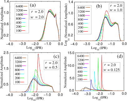
Figure 19: (Color online) Histograms are shown versus $\log_{10}(\textrm{IPR})$ for the decay power $r=2.0$ for systems ranging in size (by successive doubling) from $N=100$ to $N=6400$. Panels (a), (b), (c), and (d) correspond to $V=2.0~{},1.0,~{}0.5~{}\textrm{and}~{}0.125$, respectively.

In Fig. 19, the tunneling matrix element decreases relatively rapidly with $r=2.0$ for the decay power, and the histograms shown in panels (a), (b), (c), and (d) are consistent with the scenario in which all eigenstates are localized in the bulk limit, even for small values of $V$ or weak random potentials. In each of the panels (a), (b), (c), and (d) of Fig. 19, histogram curves corresponding to various systems sizes $N$ are shown, where the sequence of system sizes is chosen to facilitate the study of the effect of successive doubling of $N$ on the histogram profile. In panels (a) and (b), convergence to an invariant histogram curve corresponding to localized states is relatively swift, while the approach to the limiting profile is more gradual in the curves shown in panel (c), where $V=0.5$, and panel (d) with $V=0.125$. Nevertheless, the graphs in Fig. 19 indicate a stabilization of the results with respect to doubling $N$ for each random potential strength shown, and we conclude for the hopping term decay exponent $r=2.0$ that essentially any random on-site potential strength (irrespective of the strength $V$) is sufficient to localize states in the bulk limit).

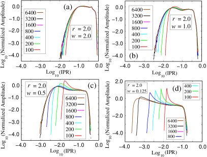
Figure 20: (Color online) Histograms with the amplitude given as a base ten logarithm are shown versus $\log_{10}(\textrm{IPR})$ for the decay power $r=2.0$ for systems ranging in size (by successive doubling) from $N=100$ to $N=6400$. Panels (a), (b), (c), and (d) correspond to $V=2.0,~{}1.0,~{}0.5,~{}\textrm{and}~{}0.125$, respectively.

For the graphs shown in Fig. 20, the vertical axis represents the base 10 logarithm of the histogram amplitude, and the random potential strengths $V$ are identical to those of the corresponding graphs in Fig. 19. A salient feature of the curves is the convergence to a profile which terminates for a particular IPR with no histogram weight above this upper limit IPR value. For sufficiently large values of the decay exponent $r$ (i.e. for at least $r\geq 2.0$), there is a minimum value $\textrm{IPR}_{\mathrm{min}}$ where the histogram amplitude abruptly falls to zero, and there is no probability of finding states with a lower IPR, a condition indicating the absolute localization of all states in the bulk limit.

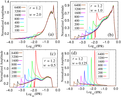
Figure 21: (Color online) Histograms are shown versus $\log_{10}(\textrm{IPR})$ for the decay power $r=1.2$ for systems ranging in size (by successive doubling) from $N=100$ to $N=6400$. Panels (a), (b), (c), and (d) correspond to $V=2.0,~{}1.0,~{}0.5,~{}\textrm{and}~{}0.125$, respectively.

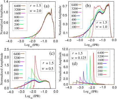
Figure 23: (Color online) Histograms are plotted versus $\log_{10}(\textrm{IPR})$ for the decay power $r=1.5$ for systems ranging in size (by successive doubling) from $N=100$ to $N=6400$. Panels (a), (b), (c), and (d) correspond to $V=2.0,~{}1.0,~{}0.5,~{}\textrm{and}~{}0.125$, respectively.

As the decay exponent $r$ is decreased, there seems to be a threshold value $r_{c}$ where the properties of the IPR histogram change in a qualitative manner with respect to increasing $N$. Fig. 21 and Fig. 22 show histogram curves for $r=1.2$, whereas Fig. 23 and Fig. 24 display IPR histograms for the case $r=1.5$ where the decay of the tunneling coefficients is faster. A salient common characteristic in the graphs obtained for $r=1.2$ and $r=1.5$ suggests both decay exponents are below the threshold value $r_{c}$. In contrast to the $r=2.0$ case, where the histogram profiles converge to a curve which does not change with successive doubling of the size $N$ (a behavior compatible with the localization of all states), for both the cases $r=1.5$ and $r=1.2$, there is a steady advance of the leftmost edge of the histogram curve toward smaller IPR values in the low-IPR regime. The size of the increment appears to be essentially the same each time the size of the system is doubled. On the other hand, for larger IPR values, the rightmost parts of the histogram converge and cease to change with increasing $N$.

The shift of the leftward edge toward lower $\log_{10}(\textrm{IPR})$ values occurs at a constant rate with doubling of the size $N$ of the system,a phenomenon seen for all of the histograms obtained for $r=1.2$ and $r=1.5$. While a bimodal structure may be seen in both the graphs obtained for $r=1.2$ and $r=1.5$, dual peaked character is most prominently manifest for the slower decay exponent $r=1.2$ and for lower values of $V$ corresponding to weaker random potentials. The two peaks behave very differently with increasing $N$. Whereas the rightmost peak, corresponding to relatively higher IPR values and hence more localized character does not shift significantly in location, the peak on the left migrates steadily toward lower IPR values with successive doubling of $N$. In addition, the peak height appears to decrease at a geometric rate each time the system size is doubled.

The curves shown in Fig. 22 and Fig. 24, where the amplitude of the IPR histogram is presented as a base 10 logarithm, highlight an important feature for the histograms in the cases $r=1.2$ and $r=1.5$ absent in the case of the more rapidly decaying scheme where, for example, $r=2.0$. For large (but finite) $N$ the log-log curves for $r<r_{c}$ may be divided, crudely speaking, into three regimes. Moving leftward along the horizontal $\log_{10}(\textrm{IPR})$ axis, one first sees a rapid rise to a maximum, and the curve then begins to decrease with decreasing $\log_{10}(\textrm{IPR})$. For intermediate values of the logarithm of the Inverse Participation Ratio, the logarithm of the histogram amplitude decreases linearly with decreasing $\log_{10}(\textrm{IPR})$. Finally, the curve rises again to reach a second maximum before beginning a rapid decline.

The intermediate regime where the logarithm of the histogram amplitude decreases linearly is a salient common feature which becomes broader as $N$ is increased (extending further and further leftward). For $r=1.2$ and $V=0.125$, the region where the dependence is approximately linear is more difficult to discern, but would be more readily seen for systems sizes beyond the largest ($N_{\mathrm{max}}=6400$) we consider in the context of this study. However, even though the linear dependence may not be readily visible, the leftward peaks in the log-log graph decrease in height at a linear rate even for weaker potentials (e.g., $V=0.125$) where the intermediate linear region is more difficult to discern. (The linear decline of the peak height in the log-log plot with successive system size doublings is compatible with the geometric decline evident in the semilogarithmic graphs.) Simple extrapolation would suggest that as the bulk limit is approached, the leftward edge of the histogram curve will continue to advance at a constant rate to the left; ultimately, in the thermodynamic limit, the asymptotically linear decrease in the logarithm of the histogram amplitude would continue for arbitrarily small $\log_{10}(\textrm{IPR})$. Hence, in terms of the histogram density $\phi_{\mathrm{IPR}}$, the support for states decreases with decreasing IPR, ultimately vanishing as the IPR heads to zero (i.e., for bona fide extended states). Although the statistical weighting decreases with decreasing IPR for all values of $r$ considered, the decline is much less abrupt if $r<r_{c}$.

In particular, we infer the explicit dependence for the IPR density $\phi_{\mathrm{IPR}}$ for $r<r_{c}$ will be $\log_{10}(\phi_{\mathrm{IPR}})=\alpha\log_{10}(\textrm{IPR})+\beta$, a relation which would hold in the bulk limit for reasonably large values of $\log_{10}(IPR)$. Inverting for $\phi_{\mathrm{IPR}}$ yields $\phi_{\mathrm{IPR}}=f(r,v)(\textrm{IPR})^{\alpha(r,v)}$, where $f(r,v)$ and $\alpha(r,v)$ depend on the hopping decay exponent $r$ and the random potential strength $V$ ($f$ would also depend on the specific type of random disorder, be it generated in a binary fashion or sampled from a uniform distribution). For fixed potential strength $V$, we anticipate that $\alpha(r,v)$ will rise sharply in the vicinity of $r=r_{c}$, where the decay of the histogram weight becomes much more rapid than for $r<r_{c}$.

The sudden shift in the behavior of the IPR histograms as the system size is successively doubled suggests an abrupt transition from the condition where the asymptotic dependence of the histogram density is a relatively slow decay with decreasing IPR, $\phi_{\mathrm{IPR}}=f(r,V)(\textrm{IPR})^{\alpha(r,v)}$ to a much more rapid decrease. The transition is likely signaled by a divergence in the exponent $\alpha$ at a critical value $r_{c}$ of the decay exponent in the extended hopping scheme.

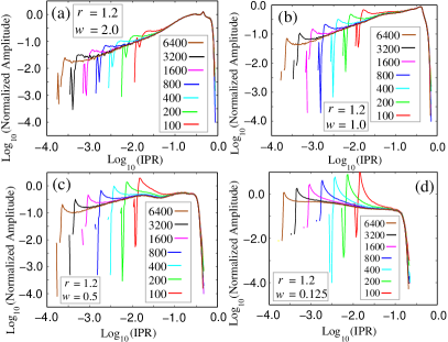
Figure 22: (Color online) Histograms with the amplitude given as a base ten logarithm are shown versus $\log_{10}(\textrm{IPR})$ for the decay power $r=1.5$ for systems varying in size (by successive doubling) from $N=100$ to $N=6400$. Panels (a), (b), (c), and (d) correspond to $V=2.0,~{}1.0,~{}0.5,~{}\textrm{and}~{}0.125$, respectively.

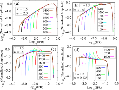
Figure 24: (Color online) Histograms with the amplitude given as a base ten logarithm are shown versus $\log_{10}(\textrm{IPR})$ for the decay power $r=1.5$ for systems ranging in size (by successive doubling) from $N=100$ to $N=6400$. Panels (a), (b), (c), and (d) correspond to $V=2.0,~{}1.0,~{}0.5,~{}\textrm{and}~{}0.125$, respectively.

IV Conclusion

We have shown with numerical calculations and analytical results that (1D) tight-binding models with on-site disorder and higher-order hopping terms exhibit interesting and non-trivial localization phenomena that can vary considerably from the well-known results of the nn tight-binding models. In the specific case where the on-site potential is an incommensurate potential (particularly the bi-chromatic problem), we have shown that for a general expression for the decay in the hopping terms with range, the energy-dependent mobility edges can be predicted approximately based on the ratio of the nn and nnn hopping terms, $t_{1}/t_{2}$, for sufficiently fast decay.

We have also considered the case of bounded, uncorrelated disorder, where we have shown that in the examined models, the higher order hopping terms can remove the symmetry in the localization length about the energy band center compared to the nn Anderson model. Broadly speaking, it appears that eigenstates with lower energies tend to localize with shorter localization lengths (i.e. higher IPR values) compared to higher-energy eigenstates due to the presence of the higher-order hopping terms.

There is also the curious case of inverse-power-law hopping terms where a mobility edge may manifest itself at the top band edge if the decay exponent is smaller than a certain critical value.

We have prepared histograms of the IPR to determine the statistical characteristics of the IPR distribution for the model with power law decay hopping. For relatively short-range hopping schemes, the histogram weight falls to zero for finite IPR values, suggesting that all states are localized in the bulk limit. However, if the hopping terms decay sufficiently slowly with distance, the histogram density is still zero in the low IPR limit, but the decay has a much slower asymptotic dependence with the form $f(r,v)(\textrm{IPR})^{\alpha(r,v)}$.

Our results are especially relevant to current experimental efforts as we consider alternatives to solid-state systems to study quantum transport, such as cold atoms in shallow optical lattices. Such systems may not be as strongly binding as solid-state systems, and therefore, do not fit well with the nn tight-binding assumption. Given this and the considerable degree of control given to experimentalists in optical lattices, these results can be observed experimentally within cold atomic systems. In particular, the current experiments in cold atomic gases Billy et al. (2008); Roati et al. (2008) have already verified the basic (and long-established) features of 1D quantum localization properties in the Anderson and the Aubry model. Experiments in shallow lattices allowing longer-range hopping should enable a deeper understanding of the localization properties discussed in the current work.

We conclude with some discussion of some of the open questions in this subject, which may be of importance for future studies. One important issue completely beyond the scope of the current work is the effect of interaction on our predicted mobility edges in the generalized one-particle AA model. In general the solid-state experimental systems are many-particle systems, and interaction is invariably present. In atomic systems where the interaction is often short-ranged, it is possible to approach the noninteracting limit by having a very dilute system, and this is one reason behind the recent experimental success in studying localization properties in refs. Billy et al. (2008); Roati et al. (2008). It is also obvious that, while our one-electron localization theory applies both to fermions and bosons since quantum statistics are irrelevant in the single-particle limit, the many-particle interacting situation is different for fermions and bosons and must be studied independently. In principle this is a formidable task, although in one dimension progress is feasible by combining numerical and analytical methods.

The interacting bosonic problem is easier to study theoretically, and for the strict nn-hopping AA model Aubry and André (1980), the conclusion — based on extensive density-matrix-renormalization-group (DMRG) studies of the problem — appears to be that the main features of the minimal AA model is preserved although a complex phase diagram now emerges in the presence of both interaction and incommensurate potential manifesting a complex interplay between superfluid and Mott insulating phasesRoux et al. (2008); *Cai10. Such numerical studies using DMRG or perhaps the time-evolving-block-decimation (TEBD) technique should, in principle, be possible for our extended AA model, and it will be an interesting future direction to pursue in this problem. An alternative technique for studying the bosonic problem in the presence of both the incommensurate AA potential and interaction is to utilize the nonlinear Schrodinger equation approach using the so-called Gross-Pitaevski equation (GPE). Such a study has recently been carried outFishman et al. ; *Krivolapov2010; *Deissler2010; *Larcher2009 for the Anderson model in the bosonic case where the interplay of disorder and interaction was studied both numerically and analytically with the conclusion that the basic qualitative feature of the non-interacting model is not modified by the presence of interaction (i.e. all states remain localized even in the presence of interaction). Again, such a GPE-based study should, in principle, be possible for our generalized AA model, although it is likely to be numerically challenging. Based on the existing results, Roux et al. (2008); *Cai10; Fishman et al. ; *Krivolapov2010; *Deissler2010; *Larcher2009 our best guess is that our conclusion in the current work about the existence of a mobility edge in the generalized AA model in the presence of non-nearest neighbor hopping will remain valid for bosonic systems even in the presence of interaction, but more work is necessary to establish this point.

Studying the interacting system becomes much more difficult and complex for fermions where the interplay of interaction and localization is notoriously difficult to study. It is well known that in general (repulsive) interaction leads to effective delocalization since the interacting particles want to stay away from each other. On the other hand, strong interaction also causes Mott transition and Wigner crystallization (where the system becomes pinned in the presence of disorder), and thus enhances localization effects in some situations. Direct numerical diagonalization and other works for the fermionic Hubbard model in the presence of disorder Kotlyar and Das Sarma (2001); *Giamarchi1988 indicate that interaction tends to increase the localization length without modifying the basic localization properties of the 1D Anderson model. Although no detailed investigation of the AA model for fermions in the presence of interaction has yet been undertaken in the literature, it is reasonable to assume, based on the results of the corresponding interacting Anderson model, that the basic picture of the noninteracting AA model would remain valid qualitatively even in the presence of interaction. We therefore believe that the existence of mobility edges in the generalized AA model discussed in the current work will remain valid even in the presence of interaction for both bosons and fermions, but much more work will be needed to settle this issue decisively. This remains an interesting and important problem for future studies. We also mention in this context a recent work Albert and Leboeuf (2010) which draws an interesting distinction between the AA model and the Anderson model with respect to the nature of the underlying localization properties, and it will be interesting to investigate whether such an analysis sheds insight into our discovery of a mobility edge in the generalized AA model in the presence of non-nearest-neighbor hopping.