Many-body calculations of low-energy eigenstates in magnetic and periodic systems with self-healing diffusion Monte Carlo: steps beyond the fixed phase

Abstract

The self-healing diffusion Monte Carlo algorithm (SHDMC) [Reboredo, Hood and Kent, Phys. Rev. B 79, 195117 (2009); Reboredo, ibid. 80, 125110 (2009)] is extended to study the ground and excited states of magnetic and periodic systems. The method converges to exact eigenstates as the statistical data collected increases if the wave function is sufficiently flexible. It is shown that the wave functions of complex anti-symmetric eigen-states can be written as the product of an anti-symmetric real factor and a symmetric phase factor. The dimensionality of the nodal surface is dependent on whether phase is a scalar function or not. A recursive optimization algorithm is derived from the time evolution of the mixed probability density, which is given by an ensemble of electronic configurations (walkers) with complex weight. This complex weight allows the amplitude of the fixed-node wave function to move away from the trial wave function phase. This novel approach is both a generalization of SHDMC and the fixed-phase approximation [Ortiz, Ceperley and Martin, Phys Rev. Lett. 71, 2777 (1993)]. When used recursively it simultaneously improves the node and the phase. The algorithm is demonstrated to converge to nearly exact solutions of model systems with periodic boundary conditions or applied magnetic fields. The computational cost is proportional to the number of independent degrees of freedom of the phase. The method is applied to obtain low-energy excitations of Hamiltonians with magnetic field or periodic boundary conditions. The method is used to optimize wave functions with twisted boundary conditions, which are included in a many-body Bloch phase. The potential applications of this new method to study periodic, magnetic, and complex Hamiltonians are discussed.

I Introduction

Following the basic prescriptions of quantum mechanics, one could potentially calculate any physical quantity. Finding the solutions of the Schrödinger equation, the wave functions and the associated energies is all that it is required. However, the computational cost of obtaining the solutions of many-body problems is well known to increase exponentially with the number of particles. Minimizing this exponential cost by either improved algorithms or an insightful approximation is the central paradigm of condensed matter theory.

Many physical quantities (observables) are only functionals of the probability density: the square of the modulus of the wave function. Some other observables, like the ground-state energy, are only functionals of the electronic density hohenberg . However, very important quantities, such as the current density or excitonic transition matrix elements, depend critically on the wave function.

In confined systems, if the Hamiltonian has time reversal symmetry, a real-value wave function is well known to exists. However, as soon as periodic boundary conditions are introduced in the Hamiltonian or a magnetic field is applied, the amplitude of the wave function is, in general, complex. If a wave function has a complex amplitude, both its modulus $\Phi({\bf R})$ and its complex phase $e^{{\bf i}\phi({\bf R})}$ can depend on the many-body coordinate ${\bf R}=\{{\bf r}_{1},{\bf r}_{2},\cdots,{\bf r}_{N_{e}}\}$, where ${\bf r}_{j}$ is the position of electron $j$ and $N_{e}$ is the number of electrons.

In addition, for fermions, the many-body wave function must change sign when the coordinates of any pair ${\bf r}_{j}$, ${\bf r}_{k}$ are interchanged in ${\bf R}$. In principle, if the wave function is real-valued, one only needs to determine the exact surface where the wave function is zero and changes sign (the node) to find the ground-state energy with diffusion Monte Carlo (DMC) methods. Any error in the determination of the node results in an overestimation of the ground-state energy anderson79 ; reynolds82 ; HLRbook .

The standard DMC method ceperley80 and improvements ortiz93 related to it require, as an input, a trial wave function $\Psi_{T}({\bf R})=\Phi_{T}({\bf R})e^{{\bf i}\phi({\bf R})}$, where both the modulus $\Phi_{T}({\bf R})$ and $\phi({\bf R})$ can be chosen to be real. The node is the surface $S_{T}({\bf R})$ in the $3N_{e}$ dimensional many-body space where $\Psi_{T}({\bf R})=0$.

The cost of a single DMC step in the standard algorithm is polynomial in the number of electrons $N_{e}$, and can be reduced to almost linear if localized orbitals are used williamson ; alfe04 ; reboredo05 . As a consequence, the existence of an algorithm that finds the required node with polynomial cost in $N_{e}$ has been subject of controversy ceperley91 ; mtroyerprl2005 . It has been argued that one of the most important problems in many-body electronic structure theory is to accurately find representations of the fermion nodes ceperley91 ; mtroyerprl2005 , which could help in solving the so-called “fermion sign problem.”

In general, a guess of the node $S_{T}({\bf R})$ and the phase $\phi({\bf R})$ can be obtained from mean field or quantum chemistry methods [such as density functional theory (DFT), Hartree-Fock, or configuration interaction (CI)]. This initial trial wave function is often improved using various methods mfoulkesrmp2001 ; ortiz95 ; jones97 ; guclu05 ; umrigar07 within a variational Monte Carlo (VMC) context. This standard approach depends on the accidental accuracy of the mean field to find the node or the possibility to perform accurate CI calculations to pre-select a multideterminant expansion for $\Psi_{T}({\bf R})$. In addition, it can be claimed that a variational optimization of the trial wave function energy or its energy variance only improves the nodes indirectly luchow07 .

In the last two years, we have developed a method to circumvent the sign problem for the ground and low-energy eigenstates of confined systems keystone ; rockandroll . This method was recently validated in real molecular systems rollingstones . We called the method self-healing diffusion Monte Carlo (SHDMC) since the nodes are corrected in a DMC context (as opposed to a VMC optimization) and the wave function converges to nearly exact keystone or state-of-the-art solutions rollingstones , even starting from random. This approach is based on the proof keystone that by locally smoothing the discontinuities in the gradient of the fixed-node ground state $\Psi_{FN}({\bf R})$ at $S_{T}({\bf R})$, a new trial wave function can be obtained with improved nodes. This proof enables an algorithm that systematically moves the nodal surface fn:sampling $S_{T}({\bf R})$ towards that of an eigenstate. The trial wave function is self-corrected within a recursive DMC approach. If the form of trial wave function is sufficiently flexible and given sufficient statistics, the process leads to an exact eigenstate many-body wave function keystone ; rockandroll ; rollingstones .

The success of the fixed-node approximation anderson79 used in the standard DMC algorithm for real wave functions is related to the quadratic dependence of the error in the fixed-node energy with the distance between $S_{T}({\bf R})$ and the exact node HLRbook $S({\bf R})$. Because the probability density goes to zero quadratically at $S({\bf R})$, errors due to small and short wave-length departures of $S_{T}({\bf R})$ from $S({\bf R})$ do not propagate far into the nodal pocket. Since the DMC energy is dominated by the average far from the node, DMC tolerates short wave-length departures of $S_{T}({\bf R})$ around $S({\bf R})$.

However, if the amplitude of wave function is complex, one must also determine its phase $\phi({\bf R})$. The ground-state energy of complex wave functions can be calculated within the fixed-phase approximation ortiz93 of DMC (FPDMC). But any error in the phase also results in an overestimation of the ground-state energy even if the exact nodes are provided ortiz93 . For complex wave functions, moreover, the error in the phase can be more dramatic than the nodal error, since the gradient of phase ${\bf\nabla}\phi({\bf R})$ is sampled everywhere, and in particular in the regions of large probability density (see below and Ref. ortiz93, ).

Since (i) periodic or infinite systems are dominant in solid state physics, (ii) the ability to calculate complex-valued wave functions (with current) is crucial to understanding transport, (iii) the response of quantum systems to magnetic fields is key for basic understanding of correlated phenomena and even applications such quantum computation, (iv) most physical systems of interest are not confined, and (v) the error in the phase affects the result more than the error in the node, solving “the phase problem” is, perhaps, as important as solving the sign problem.

In this paper a method is derived to simultaneously obtain not only the node but also the complex amplitude of the trial wave function for lower energy eigenstates of Hamiltonians with periodic boundary conditions or under applied magnetic fields. It is shown that if the phase of the wave function is a scalar function, there is a ‘special’ gauge transformation of the many-body Hamiltonian where the wave functions is real. These wave functions have nodes that are optimized as in original SHDMC method. If the phase can only be expressed by multi-valuate function, the nodal surface may have a reduced dimensionality but there is no constraint to update the wave-function in SHDMC if the nodes are removed.

The method is applied and validated in a model system studied previously rosetta where near-analytical solutions can be obtained. The scaling of the cost of this new approach is linear in the number of independent degrees of freedom of the phase. The method is a generalization of both the “fixed-phase” approach ortiz93 and the self-healing DMC algorithms developed to circumvent the sign problem keystone ; rockandroll ; rollingstones . The amplitude of the wave function is free to adjust to the complex weight of the walkers in a recursive approach.

A study of Refs. keystone, ; rockandroll, ; rollingstones, in reverse chronological order (with increasing detail) is recommended before reading this article. Studying again the seminal fixed-phase paper by Ortiz, Ceperley and Martin (OCM) ortiz93 and the importance sampling method by Ceperley and Alder ceperley80 is also highly encouraged.

The rest of the paper is organized as follows: In Section II, the SHDMC and FPDMC methods are generalized and blended into a new algorithm that optimizes the complex amplitude (and, if there is one, the node) of the trial wave function within a DMC approach. As in the case of SHDMC, the trial wave function is adjusted recursively within a generalized DMC approach. In Section III, the generalization of SHDMC is applied to a model Hamiltonian with periodic boundary conditions. The results are compared with converged CI results for the same model. In Section IV, the Zeeman splittings of the ground and excited states of a model system are calculated and compared with converged CI results. Section V describes the results obtained with a realistic Coulomb interaction. Finally, Section VI discusses the advantages, perspectives, and possible applications of these methods for many-body problems.

II A free-amplitude recursive diffusion Monte Carlo method

This section shows how one can obtain an improved trial wave function $\Psi_{T}({\bf R},\tau(\ell+1))=\langle{\bf R}|\Psi_{T}^{\ell+1}\rangle$ by applying a smoothing operator $\hat{D}$ and an evolution operator $e^{-\tau\hat{\mathcal{H}}_{FN}^{\ell}}$ (during a small imaginary time $\tau$) to the trial wave function $\Psi_{T}({\bf R},\tau\ell)=\langle{\bf R}|\Psi_{T}^{\ell}\rangle$ provided before. The limit $\tau^{\prime}=\ell\tau\rightarrow\infty$ is reached recursively as the iteration index $\ell\rightarrow\infty$.

Following the seminal ideas of OCM ortiz93 , $\Psi_{T}({\bf R},\tau^{\prime})$ can be written fn:taup as an explicit product of a complex phase and an amplitude $\Psi_{T}({\bf R},\tau^{\prime})=\Phi_{T}({\bf R})e^{{\bf i}\phi({\bf R})}$. OCM chose $\Phi_{T}({\bf R})$ to be symmetric (bosonic like), real, and positive, while the phase factor $e^{{\bf i}\phi({\bf R})}$ was antisymmetric for particle exchanges. However, the symmetry of a the phase factor is arbitrary: a symmetric phase factor can be obtained as

$$e^{{\bf i}\phi({\bf R})}=\left[\frac{\Psi_{T}({\bf R},\tau^{\prime})}{\Psi_{T}^{*}({\bf R},\tau^{\prime})}\right]^{1/2}\;,$$ (1)

since both $\Psi_{T}({\bf R},\tau^{\prime})$ and its complex conjugate change sign for particle exchanges. Therefore, any eigenstate can also be written as the product of a complex-symmetric phase factor $e^{{\bf i}\phi({\bf R})}$ (like the Jastrow factor) and a real function $\Phi_{T}({\bf R})$ where the symmetry of $\Phi_{T}({\bf R})$ depends on whether fermions or bosons are considered .

In this work it is proved (see Subsection II.1) that if the phase of a fernionic eigenstate is a scalar function, then $\Phi_{T}({\bf R})$ has the same nodal structure than real functions. Otherwise $\Phi_{T}({\bf R})$ might not be zero except for ${\bf r}_{i}={\bf r}_{j}$. Thus, the node of the trial wave function $\Psi_{T}({\bf R},\tau^{\prime})$ is given in any case by $\Phi_{T}({\bf R})$ but the dimensionality of the nodal surfaces depend on the phase.

The evolution for an additional imaginary time $\tau$ of $\Psi_{T}({\bf R},\tau^{\prime})$ is given by

$$\Psi_{T}({\bf R},\tau^{\prime}+\tau)= \;e^{-\tau\hat{\mathcal{H}}_{FN}^{\ell}}\Psi_{T}({\bf R},\tau^{\prime})$$ (2)

$$= \;e^{-\tau\hat{\mathcal{H}}_{FN}^{\ell}}\left[\Phi_{T}({\bf R})e^{{\bf i}\phi({\bf R})}\right]$$ (3)

$$= \;\Phi_{T}({\bf R},\tau)e^{{\bf i}\phi({\bf R})}.$$ (4)

Equation (4) includes all the time dependence of the wave function in $\Phi_{T}({\bf R},\tau)$, while the phase $\phi({\bf R})$ remains fixed ortiz93 .

In Eq. (2), $e^{-\tau\hat{\mathcal{H}}_{FN}^{\ell}}$ is the fixed-node evolution operator, which is a function of the fixed-node Hamiltonian operator $\hat{\mathcal{H}}_{FN}^{\ell}$ given by

$$\hat{\mathcal{H}}_{FN}^{\ell}=\hat{\mathcal{H}}+\!\infty\ \lim_{\epsilon\rightarrow 0}\theta\left\{\epsilon-d_{m}[S_{T}({\bf R^{\prime}},\ell\tau)-{\bf R}]\right\}\;.$$ (5)

The second term on the right-hand side of Eq. (5) adds an infinite potential ortiz93 at the points ${\bf R}$ with minimum distance to any point on the nodal surface $d_{m}[S_{T}({\bf R^{\prime}},\tau^{\prime})-{\bf R}]$ smaller than $\epsilon$. The fixed-node Hamiltonian is dependent on $\ell$ since the nodes $S_{T}({\bf R^{\prime}},\tau^{\prime})$ change from one iteration to the next.

In Eq. (5), the many-body Hamiltonian $\hat{\mathcal{H}}$ is given in atomic units by

$$\hat{\mathcal{H}}=\sum_{j}^{N_{e}}\frac{(\nabla_{j}+{\bf A}_{j})^{2}}{2}+V({\bf R})-E_{T}$$ (6)

where ${\bf A}_{j}={\bf A}({\bf r}_{j})$ is a vector potential at point ${\bf r}_{j}$, $V({\bf R})$ includes the electron-electron interaction and any external potential, and $E_{T}$ is a complex fn:gauge energy reference, adjusted to normalize the projected wave function, that cancels out any phase shift resulting from arbitrary gauge choices for ${\bf A}_{j}$ (see remarks below).

Using Eq (2), one can easily obtain

$$\frac{d}{d\tau}\left[\Phi_{T}({\bf R},\tau)\right]= -e^{-{\bf i}\phi({\bf R})}\hat{\mathcal{H}}_{FN}e^{-\tau\hat{\mathcal{H}}_{FN}}\Psi_{T}({\bf R},\tau^{\prime})$$

$$= -\left[E_{L}({\bf R},\tau)-E_{T}\right]\Phi_{T}({\bf R},\tau)$$ (7)

with

$$E_{L}({\bf R},\tau)= -\frac{1}{2}\!\!\sum_{j}^{N_{e}}\frac{\nabla_{j}^{2}\Phi_{T}({\bf R},\tau)}{\Phi_{T}({\bf R},\tau)}$$ (8)

$$+\frac{1}{2}\sum_{j}^{N_{e}}\left|{\bf A}_{j}+{\bf\nabla}_{j}\phi({\bf R})\right|^{2}+V({\bf R})$$

$$-{\bf i}\sum_{j}^{N_{e}}\left\{\frac{{\bf\nabla}_{j}\Phi_{T}({\bf R},\tau)}{\Phi_{T}({\bf R},\tau)}.\left[{\bf A}_{j}\!+\!{\bf\nabla}_{j}\phi({\bf R})\right]\right.$$

$$\;\;\;\;\;\;\;\;\;\;\;\;\;+\left.\frac{{\bf\nabla}_{j}\cdot\left[{\bf A}_{j}+{\bf\nabla_{j}}\phi({\bf R})\right]}{2}\right\}.$$

In Eq. (II), $E_{L}({\bf R},\tau)$ can be a real constant only if $\Phi_{T}({\bf R})e^{{\bf i}\phi({\bf R})}$ is an eigenstate of $\hat{\mathcal{H}}_{FN}$. In general, for an arbitrary trial wave function, $E_{L}({\bf R},\tau)$ is a complex function of ${\bf R}$. The real part of $E_{L}({\bf R},\tau)$ is given by the first three terms in Eq. (8), while the imaginary contribution is given by the last one. OCM’s fixed-phase approximation results from considering only the real part fn:fixed_phase of $E_{L}({\bf R},\tau)$. With little effort, one can obtain Eq. (3) of OCM’s work assuming $Im[E_{L}({\bf R})]=0$, which leads to a continuity-like equation for fluids.

Note that if $\phi({\bf R})$ is held fixed and $Im[E_{L}({\bf R})]\neq 0$ [see Eqs. (2), (4), (II), and (8)], then $\Phi_{T}({\bf R},\tau)$ must not only change its modulus but also must be free to drift away from the real values as $\tau$ increases.

If at $\tau=0$ an initial distribution of $N_{w}$ walkers $f({\bf R},0)$ is generated to be equal to $N_{w}|\Phi_{T}({\bf R})|^{2}$, within a generalization of the importance sampling algorithm of Ceperley and Alder ceperley80 (see below), $f({\bf R},\tau)$ should evolve in imaginary time as

$$f({\bf R},\tau) =\Phi_{T}({\bf R})\Phi_{T}({\bf R},\tau).$$ (9)

Clearly $f({\bf R},\tau)$ can be complex for $\tau>0$ if $Im[E_{L}({\bf R},\tau)]~{}\neq~{}0$ [see Eq. (II)].

Replacing Eq. (II) into Eq. (9), and following a procedure almost identical to the one used in Ref. ceperley80, , one obtains

$$\left.\frac{\partial f({\bf R},\tau)}{\partial\tau}\right|_{\tau\approx 0}= \frac{1}{2}\sum_{j}^{N_{e}}\left\{\nabla_{j}^{2}f({\bf R},\tau)-{\bf\nabla}_{j}\cdot\left[f({\bf R},\tau){\bf F}_{Q}^{j}\right]\right\}$$

$$-\left[E_{L}({\bf R})-E_{T}\right]f({\bf R},\tau),$$ (10)

where

$${\bf F}_{Q}^{j}={\bf\nabla}_{j}ln\left|\Phi_{T}({\bf R})\right|^{2}\;,$$ (11)

and $E_{L}({\bf R})=E_{L}({\bf R},0)$ is the complex local energy constructed using Eq. (II). To obtain Eq. (10) one must to assume that

$$\frac{{\bf\nabla}_{j}\Phi_{T}({\bf R},\tau)}{\Phi_{T}({\bf R},\tau)}\simeq\frac{{\bf\nabla}_{j}\Phi_{T}({\bf R})}{\Phi_{T}({\bf R})},$$ (12)

which implies that unlike the standard DMC algorithm ceperley80 , there is an error in Eq. (10) when $\tau\rightarrow\infty$ if $\Psi_{T}({\bf R},\tau)$ is not an eigenstate. This is only an apparent limitation since (i) $\tau$ at first can be made as small as required for Eq. (12) to be valid, (ii) $\tau$ can be increased later as the wave function improves and converges to an eigenstate, (iii) the limit $\tau^{\prime}\rightarrow\infty$ is reached by applying this free-amplitude method recursively (see below), and (iv) $\tau$ is already limited to be small in SHDMC with correlated sampling so that the weights remain close to $1$ (see below).

Although Eq. (10) above for $f({\bf R},\tau)$ is identical to Eq. (1) in Ref. ceperley80, , it now has a slightly more complex interpretation as a stochastic process. Each member of an ensemble of systems (walker) undergoes (i) a random diffusion caused by the zero-point motion and (ii) drifting by the trial quantum force $ln\left|\Phi_{T}({\bf R})\right|^{2}$ [which depends only on $\Phi_{T}({\bf R})$ and not on the phase], but in variance with Ref. ceperley80, , (iii) each walker carries a complex phase. In a nonbranching algorithm, the complex weight of the walkers is multiplied by $\exp\{-\left[E_{L}({\bf R})-E_{T}\right]\delta\tau\}$ at every time step.

Similar to the case of the “simple” SHDMC algorithm (see Refs. keystone, ; rockandroll, ; rollingstones, for details), the weighted distribution of the walkers can be written as

$$f({\bf R},\tau) =\lim_{N_{c}\rightarrow\infty}\frac{1}{N_{c}}\sum_{i=1}^{N_{c}}W_{i}^{j}(k)\delta\left({\bf R-R}_{i}^{j}\right).$$ (13)

In Eq. (13), ${\bf R}_{i}^{j}$ corresponds to the position of the walker $i$ at step $j$ of $N_{c}$ equilibrated configurations. The complex weights $W_{i}^{j}(k)$ are given by

$$W_{i}^{j}(k)=e^{-\left[E_{i}^{j}(k)-E_{T}\right]\tau}$$ (14)

with

$$E_{i}^{j}(k)=\frac{1}{k}\!\sum_{\ell=0}^{k-1}E_{L}({\bf R}_{i}^{j-\ell}),$$ (15)

where $E_{T}$ in Eq. (14) is now a complex energy reference periodically adjusted so that $\sum_{i}W_{i}^{j}(k)\approx N_{c}$ and $\tau$ is $k\delta\tau$ ($k$ is a small number of steps and $\delta\tau$ is a standard DMC time step).

The trial wave function $\Psi_{T}({\bf R},\tau^{\prime}+\tau)$ for the next iteration can be obtained as follows: All wave functions can be expanded in a basis as

$$\Psi_{T}({\bf R},\tau^{\prime}) =e^{J({\bf R})}\sum_{n}^{\sim}\lambda_{n}(\tau^{\prime})\Phi_{n}({\bf R}).$$ (16)

In Eq. (16), $\sum_{n}^{\sim}$ represents a truncated sum, $\{\Phi_{n}({\bf R})\}$ forms a complete orthonormal basis of the antisymmetric Hilbert space fn:basis , and $e^{J({\bf R})}$ is a symmetric Jastrow factor. The $\lambda_{n}(\tau^{\prime})$ are complex coefficients to be defined [see Eq. (24)]. Note that the expressions fn:taup

$$\Phi_{T}({\bf R}) =\pm\sqrt{\Psi_{T}({\bf R},\tau^{\prime})\Psi_{T}^{*}({\bf R},\tau^{\prime})},\text{ and }$$ (17)

$$\phi({\bf R}) =\ln[\Psi_{T}({\bf R},\tau^{\prime})/\Psi_{T}^{*}({\bf R},\tau^{\prime})]/(2i)+\pi n$$ (18)

allow the computation of all the quantities involved in $E_{L}({\bf R})$ in terms of gradients and Laplacians of $\Phi_{n}({\bf R})$ and $J({\bf R})$. In Eq. (18) $n$ is an arbitrary integer that changes the Riemann branch of the natural logarithm $\ln$, but does not contribute to the gradient within a branch. The local energy is thus independent on the choice of $n$ but at the Riemann cuts where, sometimes, $n$ has to change to make the phase continuous. However, the probability of a walker to touch the Riemann cut is, in practice, zero.

From Eqs. (2), (9) and (13), one can formally obtain

$$\tilde{\Psi}_{T}({\bf R},\tau^{\prime}+\tau)= \;e^{{\bf i}\phi({\bf R})}f({\bf R},\tau^{\prime}+\tau)/\Phi_{T}({\bf R})$$ (19)

$$= \;\langle{\bf R}|e^{-\tau\hat{\mathcal{H}}_{FN}}|\Psi_{T}(\tau^{\prime})\rangle\;.$$ (20)

The local smoothing operator is defined as

$$\langle{\bf R}^{\prime}|\hat{D}|{\bf R}\rangle =\tilde{\delta}\left({\bf R^{\prime},R}\right)$$ (21)

$$=\sum_{n}^{\sim}e^{J({\bf R^{\prime}})}\Phi_{n}({\bf R^{\prime}})\Phi_{n}^{*}({\bf R})e^{-J({\bf R})}.$$

Applying Eq. (21) to both sides of Eq. (19), using Eq. (13), and integrating over ${\bf R}$, one can easily obtain

$$\Psi_{T}({\bf R},\tau^{\prime}+\tau)= \;\langle{\bf R}|\hat{D}e^{-\tau\hat{\mathcal{H}}_{FN}}|\Psi_{T}(\tau^{\prime})\rangle$$ (22)

$$= \;e^{J({\bf R})}\sum_{n}^{\sim}\langle\lambda_{n}(\tau^{\prime}+\tau)\rangle\Phi_{n}({\bf R}),$$ (23)

with

$$\langle\lambda_{n}(\tau^{\prime}\!+\!\tau)\rangle=\frac{1}{\mathcal{N}}\sum_{i}^{N_{c}}W_{i}^{j}(k)e^{-J({\bf R}_{i}^{j})}\frac{\Phi^{*}_{n}({\bf R}_{i}^{j})}{\Psi^{*}_{T}({\bf R}_{i}^{j},\tau^{\prime})}\gamma({\bf R}_{i}^{j})$$ (24)

where $\mathcal{N}=\sum_{i=1}^{N_{c}}e^{-2J({\bf R}_{i}^{j})}$ normalizes the Jastrow factor. $\gamma({\bf R})$ is the standard time-step correction [Eq. (33) in Ref. umrigar93, ]:

$$\gamma({\bf R})=\frac{-1+\sqrt{1+2|{\bf v}|^{2}\tau}}{|{\bf v}|^{2}\tau}\text{ with }{\bf v}=\frac{\nabla\Phi_{T}({\bf R})}{\Phi_{T}({\bf R})}.$$ (25)

Note that $\Phi_{T}({\bf R})$ includes a Jastrow factor, thus Eq. (26) reduces to the one used in the original “simple” SHDMC algorithm keystone ; rockandroll for $\phi({\bf R})=0$.

In addition, as suggested by Umrigar umrigar_private for the ground-state SHDMC algorithm keystone , correlated sampling can be used also for walkers with complex weight. One can sample $\delta\lambda_{n}=\lambda_{n}(\tau^{\prime}+\tau)-\lambda_{n}(\tau^{\prime})$, which results in

$$\langle\lambda_{n}(\tau^{\prime}+\tau)\rangle=\lambda_{n}(\tau)+\langle\delta\lambda_{n}\rangle$$ (26)

$$\langle\delta\lambda_{n}\rangle=\frac{1}{\mathcal{N}}\sum_{i=1}^{N_{c}}e^{-J({\bf R}_{i}^{j})}\frac{\Phi_{n}^{*}({\bf R}_{i}^{j})}{\Psi^{*}_{T}({\bf R}_{i}^{j},\tau^{\prime})}[W_{i}^{j}(k)-1]\gamma({\bf R}_{i}^{j}).$$

These new $\lambda_{n}(\tau^{\prime}+\tau)$ [Eq. (26)] are used to construct a new trial wave function [Eq. (16)] recursively within DMC. Equation (24) can be related to the maximum-overlap method used for bosonic wave functions reatto82 .

The error of $\langle\delta\lambda_{n}\rangle$ is obtained by sampling

$$\langle\delta\lambda_{n}^{2}\rangle=\frac{1}{\mathcal{N}}\sum_{i=1}^{N_{c}}\left|e^{-J({\bf R}_{i}^{j})}\frac{\Phi_{n}^{*}({\bf R}_{i}^{j})}{\Psi^{*}_{T}({\bf R}_{i}^{j})}[W_{i}^{j}(k)-1]\gamma({\bf R}_{i}^{j})\right|^{2}.$$ (27)

The truncation of the expansion of the delta function [Eq. (21)] is a key ingredient in SHDMC since it decides how local is the smoothing operator $\hat{D}$ and prevents noise to ruin the quality of the trial wave function. If the absolute value of the error of $\langle\delta\lambda_{n}\rangle$ is larger than $|\lambda_{n}(\tau^{\prime}+\tau)|/4$, the algorithm sets $\lambda_{n}(\tau^{\prime}+\tau)$ equal to zero [which defines the truncation criterion used in the sums ($\sum_{n}^{\sim}$) involved in Eqs. (16), (21) and (22)]. See Ref. keystone, for a detailed theoretical justification of the truncation procedure and the algorithm used. Briefly here, the coefficients $\lambda_{n}$ are sampled at the end of each sub-block of $k$ DMC steps. Statistical data is collected for number of sub-blocks $M$ before a wave function update. At first, $M$ is set to a small number and increased according to the recipe given in Ref. rockandroll, . In short, the algorithm detects automatically the dominance of noise when the projection of two successive sets of $\langle\delta\lambda_{n}\rangle$ becomes small and multiplies by a factor larger than 1 the number of sub-blocks $M$ (see Ref. rockandroll, for more details). As a result, the total number of configurations $N_{c}$ sampled increases as the algorithm progresses. Therefore the statistical error is reduced, and the number of basis functions retained in the expansion increases over time. Thus, the smoothing operator $\hat{D}$ tends to the delta function as $M$ increases, which allows the SHDMC method to sample the wave function with increasing detail. The first quarter of the data in each block, following a wave function update, is discarded.

In practice, the only difference between this new approach and the original SHDMC method is the complex weight and the limitation for propagation to small $\tau$. Therefore, a nonbranching algorithm for small $\tau$ has been used (see Ref. rockandroll, for details). However, there are some formal differences on the justification of the convergence of the SHDMC method that are discussed in the next subsections.

II.1 Gauge transformations and nodal structure of complex eigenstates

The phase $\phi({\bf R})$ must be continuous at any point of ${\bf R}$ where $\Psi_{T}({\bf R})\neq 0$. Otherwise, if $\phi({\bf R})$ is not continuous, its gradient in the local energy will introduce an effective infinite potential at the discontinuity that will force $\Psi_{T}({\bf R})=0$. In some cases, however, these discontinuities in the phase are not physicalfn:discont and they can be removed by changing the Riemann sheet index $n$ in Eq. (18). As a consequence, the wave functions can be split into two classes. In the first class different Riemann sheets of $\phi({\bf R})$ are not connected. In that case, one can choose as phase a single sheet of the Riemann surface The phase in this class can be a continuous scalar function of ${\bf R}$ for every ${\bf R}$. The real wave functions, with constant phase, are special case of this class. In the second class, the Riemann surfaces of $\phi({\bf R})$ for different $n$ are connected at the Riemann cuts. Thus a continuous $\phi({\bf R})$ can only be described by a multi-valuate function of ${\bf R}$.

Eigenstates with a scalar phase: Since ${\bf\nabla}_{j}\times{\bf\nabla}_{j}\cdot\Lambda({\bf R})=0$ for any scalar function $\Lambda({\bf R})$, the magnetic field ${\bf B}={\bf\nabla}_{j}\times{\bf A}_{j}$ is invariant for the gauge transformations jackson ${\bf A}^{\prime}_{j}={\bf A}_{j}+{\bf\nabla}_{j}[\Lambda({\bf R})+c(\tau)]$, where $\Lambda({\bf R})$ is an arbitrary symmetric scalar function of ${\bf R}$ and $c(\tau)$ is an arbitrary function of $\tau$ (independent of every ${\bf r}_{j}$ in ${\bf R}$). If $\Psi_{T}({\bf R})$ is selected to be an eigenstate of $\hat{\mathcal{H}}$ for a given gauge and if $\phi({\bf R})$ is a scalar function , then a change in gauge ${\bf A}_{j}+{\bf\nabla}_{j}\delta\Lambda({\bf R})$ could be readily compensated in the phase by

$$\tilde{\phi}(\bf R)=\phi({\bf R})-\delta\Lambda({\bf R})+c(\tau),$$ (28)

without affecting $\Phi_{T}({\bf R})$ [since ${\bf A}_{j}$ and ${\bf\nabla}_{j}\phi({\bf R})$ always appear added in Eq. (8)]. This property is particularly important, since implies that for this class of eigenstates of $\hat{\mathcal{H}}$ there is a ‘special’ gauge where the wave function is real.

Note that if one sets $\delta\Lambda({\bf R})=\phi({\bf R})$ in Eq. (28) then $\tilde{\phi}(\bf R)~{}=~{}0$. Therefore, the new phase is a constant that can be chosen to be zero. The vector potential in this special gauge is a many-body object which includes the gradient of the many-body phase of the wave function in a single particle gauge.

The norm $\Phi({\bf R})$ is invariant since the effective potential in Eq. (8) is invariant using Eq. (28). This is expected since the expectation value of an arbitrary operator $\hat{\mathcal{O}}({\bf R})$ must be independent of the gauge choice for non-degenerate eigenstates. In particular, the nodes, which are given by $\Phi({\bf R})$, are also invariant to gauge transformations. Since the new phase is a constant, it can be easily shown that in the special gauge, the amplitude of those eigenstates has the same structure as the trial wave function used in the fixed-node approximation for real wave functions.

SHDMC self adjusts to an arbitrary gauge change $\delta\Lambda({\bf R})$ because $\phi({\bf R})$ is modified recursively by a change in the local energy in Eq. (8) of the form

$$\delta E_{L}({\bf R},\tau)=$$ (29)

$$\sum_{j}^{N_{e}}\left\{Re\left[\left({\bf A}_{j}+{\bf\nabla}_{j}\phi({\bf R})\right)\cdot{\bf\nabla_{j}}\delta\Lambda({\bf R})\right]+\frac{1}{2}|{\bf\nabla}_{j}\delta\Lambda({\bf R})|^{2}\right\}$$

$$-\;{\bf i}\sum_{j}^{N_{e}}\left\{\frac{{\bf\nabla}_{j}\Phi_{T}({\bf R},\tau)}{\Phi_{T}({\bf R},\tau)}\cdot{\bf\nabla_{j}}\delta\Lambda({\bf R})+\frac{1}{2}\nabla^{2}_{j}\delta\Lambda({\bf R})\right\}.$$

Eigenstates with a multi-valuate phase: On the other hand if $\phi({\bf R})$ is not a scalar function then, ${\bf\nabla}_{j}\times{\bf\nabla}_{j}\cdot\phi({\bf R})\neq 0$ and, therefore, ${\bf\nabla}_{j}\cdot\phi({\bf R})$ cannot be included in the vector potential without introducing an artificial many-body magnetic field. In that case, as pointed out timely by an anonymous referee, there might be nodes only where ${\bf r}_{j}={\bf r}_{k}$. Eigenstates with this type of nodes, with reduced dimensionality, can be found in states with current, degeneracy or magnetic fields.

Sumarizing, the norm of the complex wave-functions of the eigenstates that have a scalar phase in ${\bf R}$ has the same structure as the real wave function used in the fixed-node approach because there is a special gauge transformation where the wave function is real valued. This property has a formal importance since it allows extending theorems developed in the context of the fixed-node approximation. Instead, if different Riemann sheets of $\phi({\bf R})$ are continuously connected, a continuous phase cannot be described by a single scalar function. Then dimensionality of the nodal surface might be smaller and limited to the cases in ${\bf R}$ where ${\bf r}_{j}={\bf r}_{k}$. The nodes are an obstacle for DMC; SHDMC, however, converges to eigenstates regardless of the dimensionality of the nodes (see below).

II.2 Remarks on the free-amplitude SHDMC method

Convergence of SHDMC to eigenstates: In II.1 it is shown that the wave-function of any fermionic eigenstate can be factorized into an anti-symmetric real function $\Phi_{T}({\bf R})$, with nodes, and a symmetric phase factor (See Eq. (1)). The dimensionality of the nodal surface depends on the phase properties. Since the amplitude can not change at the node in DMC, nodes are the obstacle to overcame by SHDMC. Convergence is not affected if the initial trial wave function has no nodes because, in this case, the amplitude and the phase can evolve with $\tau$ everywhere. Indeed, SHDMC can be started from a linear combination of real and imaginary parts with different nodes. As noted by a referee, in this class of functions two particles can exchange without crossing a node. However, the convergence of SHDMC is not affected in theory and it is not affected in practice. But, if the phase is a scalar function, nodes will develop as the trial wave function converges to an eigenstate. In that limit, a kink at the node should appearkeystone until the exact node is found.

The convergence of the SHDMC approach when the trial wave function approaches an eigenstate and shows nodes, is based on the proof keystone that locally smoothing the kinks of the fixed-node wave function improves the nodes. This proof can be trivially extended to a complex wave function (when $Im[E_{L}({\bf R})]\neq 0$ ), breaking the time evolution into a sequence of pure real evolution followed by an imaginary evolution. If one assumes $Im[E_{L}({\bf R})]=0$, the present approach reduces to SHDMC method, but using the effective potential of the fixed-phase Hamiltonian ortiz93 . Thus the best nodes in $\Phi_{T}({\bf R},\tau)$ for a given phase $\phi({\bf R})$ can be obtained by running SHDMC in a fixed-phase stage. It is trivial to show that the phase, in turn, improves if the imaginary contribution is allowed to evolve a short time from a trial wave function with optimal nodes. In principle, a SHDMC fixed-phase stage can be propagated to infinite imaginary time $\tau$ within a branching algorithm. The evolution of the phase, instead, is limited to short times [for Eq. (12) to be valid]. In this work, however, the real and the imaginary parts of the wave function are allowed to evolve simultaneously during a short time without any observed adverse effect on the accuracy.

Phase and nodal errors: Note in Eq. (8) that as in the fixed-phase approach ortiz93 , an effective potential $\left|{\bf\nabla}_{j}\phi({\bf R})+{\bf A}_{j}\right|^{2}$ is added to $V({\bf R})$, which depends in turn on ${\bf\nabla}\phi({\bf R})$ and ${\bf A}_{j}$. Thus small errors in the phase $\phi({\bf R})$ have a global impact [in particular far from the node, where $|\Phi_{T}({\bf R})|^{2}>>0$]. In contrast, small errors in $\Phi_{T}({\bf R})$ only slightly displace the node and have smaller impact on the energy HLRbook [since the local energy is seldom sampled because $\lim\Phi_{T}({\bf R})\Phi_{T}({\bf R},\tau)\rightarrow 0$ at $S_{T}({\bf R})$]. For eigenstates without nodal surfaces the phase is the sole source of error. SHDMC provides a method to correct both the phase and the nodal error.

Complex $E_{T}$: Note that when $c(\tau)$ is changed in Eq. (28), it just changes the normalization of $\Psi_{T}({\bf R})$ and, if complex, introduces a global phase shift; however, $c(\tau)$ does not affect the local energy or other observables.

For a random trial wave function $\Psi_{T}({\bf R})$ and an arbitrary choice of gauge for ${\bf A}_{j}$, $E_{L}({\bf R},\tau)$ will have both real and imaginary components. The average over the walkers‘ positions will have a real contribution, which affects the norm, and a complex contribution, which introduces a global phase shift. The average of $E_{L}({\bf R},\tau)$ only contributes to $c(\tau)$. The correlated sampling approach is obviously more efficient when the distribution of complex weights is centered around 1 since the error in the coefficients is minimized [See Eq. 27 and use the standard expression for the variance]. $E_{T}$ in Eq. (14) is thus complex. The real part of $E_{T}$ renormalizes the wave function (that is, keeps the population of walkers constant). The imaginary part of $E_{T}$ removes the global phase shift [the average complex contribution of $E_{L}({\bf R},\tau)$ that only contributes to $c(\tau)$]. For a converged trial wave-function, $Im(E_{T})\simeq 0$.

Upper bound properties: The present approach should not be considered as a method to estimate the energy of the trial wave function but instead as a method to optimize the trial wave function before a final FPDMC calculation. However, since the real part of $E_{L}({\bf R})$ corresponds to the fixed-phase approximation, the real part of $E_{T}$ also converges to an upper bound of the ground-state energy. This upper bound can be higher than the fixed-phase approximation (if the limit of $\tau^{\prime}\rightarrow\infty$ is not reached or the basis $\{\Phi_{n}({\bf R})\}$ is too small). Therefore, a standard FPDMC calculation ortiz93 (with branching) must be performed to obtain final values for the ground-state energy.

Known limitations and solutions: The present approach is inefficient when the energy of the first excited state $E^{FP}_{1}$ of the fixed-phase Hamiltonian is too close to the ground-state energy $E^{FP}_{0}$, since the coefficient of the excited state component of the trial wave function decays as $exp[-\tau(E^{FP}_{1}-E^{FP}_{0})]$. In that regime, satisfactory results can be obtained as follows: begining with a small value for $M$, keep $M$ fixed for a number of iterations until the lower energy excitations decay and, then release $M$, allowing the high energy components of the wave function to converge.

Moreover, the approximate excited-state wave functions can be calculated (see Ref. rockandroll, ) and the lowest energy linear combination can be determined with correlated function Monte Carlo jones97 , VMC umrigar07 or directly in FPDMC using a restricted basis of low energy states. A final alternative is to run this free-amplitude SHDMC method with larger $\tau=k\delta\tau$ but using a smaller basis given by a few approximated excited states. The excited states can be found as described in the next section.

II.3 Generalization to excited states

Earlier estimates of excited state energies in the presence of magnetic fields have been made by diagonalizing a matrix of correlation functions in imaginary time jones97 ; ceperley88 . In addition, calculations of excited states have been reported with the auxiliary field approach purwanto09 . The present algorithm, in contrast, is almost identical to the SHDMC method keystone ; rockandroll developed for the ground state and lower excitations of real wave functions. The only relevant difference with Ref. rockandroll, is the complex weight of the walkers. Thus the free-amplitude SHDMC method described above for the ground state can be generalized in a straightforward way to study excited states as in Ref. rockandroll, .

Readers are encouraged to follow a detailed theoretical justification of the excited state algorithm in Ref. rockandroll, . Here only some key steps are described [in particular, note Eqs. (31) and (32) that were omitted in Ref. rockandroll, and are relevant for a non-unitary Jastrow factor].

As in the importance sampling algorithm ceperley80 , the generalization given by Eq. (10) requires that $\Psi_{T}({\bf R},\tau^{\prime}\;+\;\tau)$ be zero only at the nodes $S_{T}({\bf R},\tau^{\prime})$ of $\Psi_{T}({\bf R},\tau^{\prime})$, being free to change both its modulus and phase elsewhere. Therefore, $\Psi_{T}({\bf R},\tau^{\prime}+\tau)$ can develop a projection into any lower energy state consistent with $S_{T}({\bf R},\tau^{\prime})$. To obtain an excited state, the wave function $\Psi_{T}({\bf R},\tau^{\prime}+\tau)$ must be projected in the subspace orthogonal to the ground state and any other excited state calculated before. In alternative approaches such as correlation function Monte Carlo ceperley88 , the orthogonality of excited states is achieved by diagonalizing a generalized eigenvalue problem. One could argue that the excited states obtained with that approach share nodal error of the ground state. One of the advantages of SHDMC is that the diagonalization of a large matrix of excitations is avoided, which makes possible the consideration of a larger number of degrees of freedom. In addition, the nodes of each excitations are found independently. But in SHDMC, unless special conditions are satisfied rockandroll , one must calculate lowerlying energy states before attempting the calculation of higher excited states.

A projector is constructed with approximated expressions of the $\nu$ eigenstates $\Psi_{\mu}({\bf R})=\langle{\bf R}|e^{\hat{J}}\breve{\Phi}_{\mu}\rangle=e^{J({\bf R})}\breve{\Phi}_{\mu}({\bf R})$ calculated earlier as

$$\hat{P}_{\nu}=e^{\hat{J}}\left[1-\sum_{\mu}^{\nu}|\breve{\Phi}_{\mu}\rangle\langle\breve{\Phi}_{\mu}^{\dagger}|\right]e^{-\hat{J}}\;\;.$$ (30)

The operator $e^{\hat{J}}$ in Eq. (30) is the multiplication by a Jastrow. For a non-unitary $e^{\hat{J}}$ the set $\{|\breve{\Phi}_{\mu}\rangle\}$ is nonorthogonal. However, the conjugate (dual) basis hoffman ; prugovecki that satisfies $\langle\breve{\Phi}_{\mu}|\breve{\Phi}_{m}\rangle=\delta_{\mu,m}$ can be obtained statistically as

$$\langle\breve{\Phi}_{\mu}|{\bf R}\rangle=\sum_{n}^{\nu}\xi_{n}^{\mu}\Phi^{*}_{n}({\bf R})$$ (31)

with

$$\xi_{n}^{\mu}=\lim_{N_{c}\rightarrow\infty}\frac{1}{\mathcal{N}}\sum_{i}^{N_{c}}\frac{W_{i}^{j}(k)}{e^{-J({\bf R}_{i}^{j})}}\frac{\Phi_{n}({\bf R}_{i}^{j})}{\Psi_{T}^{\mu}({\bf R}_{i}^{j},\tau^{\prime})}\gamma({\bf R}_{i}^{j})\;,$$ (32)

where $\Psi_{T}^{\mu}({\bf R},\tau^{\prime})$ is the trial wave function used to evaluate earlier the state $\mu$ for $\tau^{\prime}\rightarrow\infty$. Note that the exponential involving $-J({\bf R}_{i}^{j})$ moves to the denominator in Eq. (32) as compared with Eq. (24). Since $J({\bf R})$ is real, the phase of $\langle\breve{\Phi}_{\mu}|{\bf R}\rangle$ must be conjugated to the phase of $\langle{\bf R}|\breve{\Phi}_{\mu}\rangle$. The coefficients $\xi_{n}^{\mu}$ should be sampled during the final FPDMC step (i.e., when the final excited energy is sampled).

The projection of the conjugate function $\langle\breve{\Phi}_{\mu}|$ onto earlier conjugate states should also be removed to obtain $\langle\breve{\Phi}_{\mu}|=\langle\breve{\Phi}_{\mu}|\hat{P}^{T}_{\mu-1}|$ where $\hat{P}^{T}_{\nu}$ is the transpose of $\hat{P}_{\nu}$. Furthermore, statistical errors in $\langle\breve{\Phi}_{\mu}|$ can be partially filtered by inverting the overlap matrix $S_{\mu,m}=\langle\breve{\Phi}_{\mu}|\breve{\Phi}_{m}\rangle$ as

$$\langle\breve{\Phi}_{\mu}^{\dagger}|=\sum_{m}S^{-1}_{\mu,m}\langle\breve{\Phi}_{m}|\;.$$ (33)

The scalar products resulting from applying $\hat{P}_{\mu}$ in Eq. (30) are given by

$$\langle\breve{\Phi}_{\mu}^{\dagger}|\breve{\Phi}_{m}\rangle=\sum_{n}\bar{\xi}_{n}^{\mu}\lambda_{n}^{m},$$ (34)

with $\bar{\xi}_{n}^{\mu}=\sum_{\nu}S^{-1}_{\mu,\nu}\xi_{n}^{\mu}$ since $\int\Phi_{m}^{*}({\bf R})\Phi_{n}({\bf R}){\bf dR}=\delta_{n,m}.$

The extension of SHDMC to the next excited $|\Psi_{\nu+1}\rangle$ can be thought of as the recursive application of the evolution operator $e^{-k\delta\tau\hat{\mathcal{H}}^{(\ell-1)}_{FN}}$, the projector $\hat{P}$ [Eq (30)], and a smoothing operation $\hat{D}$ [see Eq. (21)] to a trial wave function $|\Psi_{T,\nu+1}^{\ell-1}\rangle$ [see Eq. (II.3)]. This procedure can be derived analytically rockandroll as follows:

$$|\Psi_{\nu+1}\rangle = \lim_{\tau\rightarrow\infty}\hat{P}\;e^{-\tau\hat{\mathcal{H}}}\hat{P}|\Psi_{T,\nu+1}^{\ell=0}\rangle$$

$$= \lim_{\ell\rightarrow\infty}\hat{P}\;\prod_{\ell}\left(e^{-(\delta\tau^{\prime}+k\delta\tau)\hat{\mathcal{H}}}\hat{P}\right)|\Psi_{T,\nu+1}^{\ell=0}\rangle$$

$$= \lim_{\ell\rightarrow\infty}\hat{P}\;\prod_{\ell}\left(e^{-\delta\tau^{\prime}\hat{\mathcal{H}}}e^{-k\delta\tau\hat{\mathcal{H}}_{FN}^{(\ell-1)}}\hat{P}\right)|\Psi_{T,\nu+1}^{\ell=0}\rangle$$

$$\simeq \lim_{\ell\rightarrow\infty}\hat{P}\prod_{\ell}\left(\tilde{D}e^{-k\delta\tau\hat{\mathcal{H}}^{(\ell-1)}_{FN}}\hat{P}\right)|\Psi_{T,\nu+1}^{\ell=0}\rangle$$

$$= |\Psi_{T,\nu+1}^{\ell\rightarrow\infty}\rangle.$$

Replacing $e^{k\delta\tau\hat{\mathcal{H}}}$ in the infinite product in the second line of Eqs. (II.3) with $e^{-k\delta\tau\hat{\mathcal{H}}^{(\ell-1)}_{FN}}$ in the third line generates the same projector keystone ; rockandroll . In turn, we proved keystone that replacing $e^{-\delta\tau^{\prime}\hat{\mathcal{H}}}$ with a large class of local smoothing operators $D$ has the same effect on the nodes. The fixed-node Hamiltonian depends on the iteration index $\ell$ because the trial wave function, the node, $E_{T}$, and the phase are different at every iteration. Finally, the norm of the projected function can be fixed by adjusting $E_{T}$ in every iteration $\ell$.

For states with inequivalent nodal pockets, special care must be taken within the algorithm to avoid systematic errors (see Ref. rockandroll for additional details about the algorithm).

III Calculations for Hamiltonians with periodic boundary conditions

Usually periodic boundary conditions in a supercell with dimensions $a_{x}$, $a_{y}$ and $a_{z}$ are set when studying crystalline systems that simulate an infinite solid. By using the Bloch Theorem ashcroft , the trial wave function at $\tau^{\prime}=\ell\tau$ can be written as the product of a many-body phaserajagopal95 times a periodic part fn:taup $\mathcal{U}({\bf R})$ as

$$\Psi_{T}({\bf R},\tau^{\prime})=e^{{\bf i}\left(\sum_{j}^{N_{e}}{\bf k\cdot r}_{j}\right)}\mathcal{U}({\bf R})$$ (36)

with

$$\mathcal{U}(\{{\bf r_{1}},\cdots,{\bf r}_{j},\cdots,{\bf r_{N_{e}}}\})=\mathcal{U}(\{{\bf r_{1}},\cdots,{\bf r}_{j}+{\bf a},\cdots,{\bf r_{N_{e}}}\})$$

for any $j$, where ${\bf a}=a_{x}n_{x}{\bf\hat{\i}}+a_{y}n_{y}{\bf\hat{\j}}+a_{z}n_{z}{\bf\hat{k}}$, with $n_{\mu}$ being arbitrary integers. $\mathcal{U}({\bf R})$, in turn, fn:taup can be written as a product of a multi-determinant expansion times a Jastrow factor. Each orbital entering each determinant in $\mathcal{U}({\bf R})$ can be expanded in plane waves that satisfy periodic boundary conditions.

The theory developed in Section II can then be applied to periodic systems by setting ${\bf A}_{j}=0$. Note, however, that since $\mathcal{U}({\bf R})$ is in general a complex function, the phase entering in $E_{L}({\bf R})$ [see Eq. 8] must include both the phase of $\mathcal{U}({\bf R})$ and the many-body Bloch phase. The resulting wave function $\Psi_{T}({\bf R},\tau^{\prime}\rightarrow\infty)$ corresponds, in general, to a state with current, and its solution can facilitate the calculation of transport problems in a many-body context krcmar08 . The many-body Bloch phase component on the trial wave function is often referred to in the literature as twisted boundary conditions tbc ; fn:tbc .

III.1 The model periodic system

Until this new development, the author had promised himself to halt calculations in small model systems rosetta ; keystone ; rockandroll . Those small model systems, however, while not very realistic, allow comparisons to be performed with fully converged CI calculations. In addition, they can be handled with symbolic programs like Mathematica, which, while computationally very slow, are an ideal environment for developing new methods and comparing the results with nearly analytical values. Therefore, small model systems provide an ideal “workbench” for testing new theories and algorithms. On the other hand, no method that fails in the simplest case has hopes of succeeding in a realistic calculation involving the more challenging Coulomb interaction with a large number of electrons. Past experience has shown, in contrast, that earlier SHDMC developments tested and developed in small models keystone could be implemented easily in realistic cases without additional complications rollingstones . Indeed, calculations using this method in QWALK wagner09 reproduced the results obtained for the triplet state of He for low magnetic fieldsjones99 starting from a random linear combination of determinants constructed with the Hartree-Fock solutions without magnetic field. All electron calculations of atomic systems with tens of electrons are currently under progress and will be published elsewhereelsewhere .

DMC calculations with a realistic Coulomb interaction in periodic systems require a supercell large enough to prevent unphysical image interactions between periodic replicas of the electrons from dominating the result. For the purpose of testing the method, however, a model electron-electron interaction can be chosen, and the system can be made as small as required for numerical convenience. For validating the method, the Hamiltonian does not need to be strictly realistic; however, one must solve the same Hamiltonian with SHDMC and an established benchmark method (CI in this case).

The model studied in this section is related to the one considered in Refs. rosetta, ; keystone, , and rockandroll, and consists of two spinless electrons in a square of side $1$. However, instead of the hard-wall boundary conditions used earlier, periodic boundary conditions are set.

Basis expansion: The ground state of the noninteracting system is degenerate. Two states with zero total momentum can be constructed by placing two electrons with opposite momenta ${\bf k}=\pm\pi{\bf\hat{\i}}$ or ${\bf k}=\pm\pi{\bf\hat{\j}}$. The basis chosen to expand the wave function is an antisymmetric combination of free-particle solutions that satisfy periodic boundary conditions, which are plane waves of the form

$$e^{2\pi{\bf i}\left[(n+1/2)x+my\right]}$$ (37)

where $|n+1/2|<6$ and $|m|<5$, which results in a two-body basis with 1516 functions.

The confining potential and the interaction potential selected do not mix the directions ${\bf\hat{\i}}$ and ${\bf\hat{\j}}$. They are given by

$$V({\bf R})=\; 4\pi^{2}\left\{\cos(2\pi x_{1})\!+\!\cos(2\pi x_{2})\!+\!\cos(2\pi y_{1})\!+\!cos(2\pi y_{2})\right.$$

$$+\left.\cos[2\pi(x_{2}-x_{1})]+\cos[2\pi(y_{2}-y_{1})])\right\}.$$ (38)

The first line of Eq. (III.1) corresponds to an external potential applied to electrons $1$ and $2$. The second line plays the role of an interaction potential that depends on the difference between the electronic coordinates.

The Jastrow factor is set to zero to facilitate the analytical calculation of the matrix elements of $V({\bf R})$, while the kinetic energy is a diagonal matrix. The exact diagonalization of the Hamiltonian matrix is the CI result. For $\hbar=1$, the energy difference units between the noninteracting ground state and first excited states is $4\pi^{2}$. Since the interaction energy in Eq. (III.1) is of the same order of magnitude as the kinetic energy, the system is in the correlated regime.

III.2 Results and discussion

Figure 1 shows the logarithm projection $L_{P}(n)=ln|\langle\Psi_{n}^{CI}|\Psi_{T}(\ell\tau)\rangle|$ of the trial wave function $|\Psi_{T}(\ell\tau)\rangle$ onto the $n$ eigenstate of the full CI solution $|\Psi_{n}^{CI}\rangle$ as a function of the recursive iteration index $\ell$. The wave function is constrained by the basis to have a many-body Bloch phase $\phi({\bf R})=\exp[{\bf i}({\bf k\cdot r}_{1}+{\bf k\cdot r}_{2})]$ with ${\bf k}=0.9\pi({\bf\hat{\i}}+{\bf\hat{\j}})$ (that is a twist angle of $1.8\pi$ tbc ; fn:tbc both in the ${\bf\hat{i}}$ and ${\bf\hat{j}}$ directions).

The initial trial wave function $|\Psi_{T}(0)\rangle$ was chosen intentionally to be of poor quality to demonstrate the strength of the method. The coefficients of $|\Psi_{T}(0)\rangle$ corresponded to a linear combination of the first 16 full CI eigenstates: $|\Psi_{T}(0)\rangle=\sum_{n}c_{n}|\Psi_{n}^{CI}\rangle$, where the coefficients $c_{n}$ are complex numbers of modulus $1/4$ and a random phase. Note that the initial trial wave function has no nodes but at the coincidental points because is a linear combination with random phase of different eigenstates of the non interacting Hamiltonian with different nodes. The calculation was run for 200 walkers with $\delta\tau=0.0004$ and $\tau=0.02$. The coefficients $\lambda_{n}$ were sampled at the end of each sub-block of $k=50$ DMC steps. At first the number of sub-blocks $M$ sampled before a wave function update was set to $20$ and increased according to the recipe given in Ref. rockandroll, and briefly in Section II. Therefore, the statistical error is reduced, and the number of basis functions retained in the expansion increases over time. As a result both the statistical error and the truncation error diminish, and the wave function continues to improve. The final iteration included $M=600$ blocks. The total optimization run cost $\approx 1.5\times 10^{5}$ DMC steps.

Figure 1 shows in increasingly lighter shading the results $L_{P}(n)$ corresponding to higher excited states. All the projections to the first 16 states start from the same value [$-\ln(4)$] by construction. The algorithm, at first, increases the projection of the lower energy states at the expense of the higher ones (thus $L_{P}(n)$ approaches zero for low $n$), while the projections with higher $n$ (in lighter gray) become smaller and their $L_{P}(n)$ is increasingly negative. As the algorithm progresses further, the projection on lower-energy excitations also starts to decay. Finally, $L_{P}(n)$ becomes increasingly negative for all states except the ground state, which approaches zero.

As the number of recursive iterations $\ell$ increases, the projection onto highly excited states becomes negligible. The values obtained for $L_{p}(n>0)$ are, therefore, dominated by statistical noise in the sampling. On the right side of Fig. 1, the convergence of the wave function is no longer limited by the initial trial wave function but by the statistical noise. Statistical noise introduces a projection into higher excited states by two mechanisms: (i) the coefficients $\lambda_{n}$ of the trial wave function expansion include random noise and (ii) the trial wave function develops a projection into excited states because it is truncated depending on the relative error of $\lambda_{n}$, which in turn depends on $N_{c}$ keystone ; rockandroll . Accuracy can be increased only by improving the statistics (increasing $M$ and $N_{c}$).

The residual projection of the trial wave function $|\Psi_{T}(\ell\tau)\rangle$ for iteration $\ell$ on the CI eigenstate $|\Psi_{n}^{CI}\rangle$ is defined as

$$L_{rp}^{n}=\ln\left(1-|\langle\Psi_{n}^{CI}|\Psi_{T}(\ell\tau)\rangle|\right).$$ (39)

The final value for the residual projection for the calculation in Fig. 1 is below $-7$. The value obtained for the SHDMC energy is -31.842(13) as compared with a CI value of $-31.9486$. However, the SHDMC wave function retains only $70$ coefficients in the expansion, whereas the CI has $1516$. The FPDMC energy obtained with this wave function was $-32.00(2)$.

The results shown in Figure 1 demonstrate that the SHDMC method with complex weights is able to correct both the phase and the nodal structure of the trial wave function. SHDMC converges to the ground-state even starting from a poor quality wave function with a random phase.

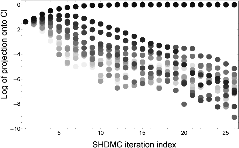
Figure 1: Logarithm of the projection of the trial wave function into the lowest 16 eigenstates obtained with CI [$L_{P}(n)=ln|\langle\Psi_{n}^{CI}|\Psi_{T}(\ell\tau)\rangle|$] as a function of the SHDMC iteration index $\ell$. The results correspond to two electrons in the triplet state with periodic boundary conditions and a many-body Bloch phase $\phi({\bf R})=\exp[{\bf i}({\bf k\cdot r}_{1}+{\bf k\cdot r}_{2})]$ with ${\bf k}=0.9\pi({\bf\hat{\i}}+{\bf\hat{\j}})$ (that is a twist angle of $1.8\pi$ tbc ; fn:tbc ). Darker symbols correspond to the projection with lower energy CI eigenstates. The initial trial wave function was a linear combination of the lowest 16 CI eigenstates with coefficients having the same modulus and a random complex phase.

III.3 Many-body band structure

Common electronic structure methods are based on a single-particle picture, and the band structure is given by the evolution of the energy as a function of the single-particle crystalline momentum. In this case, in contrast, the energy of many-body states is a function of the many-body Bloch phase $e^{{\bf i}\left(\sum_{j}^{N_{e}}{\bf k\cdot r}_{j}\right)}$ or the twist angle tbc ; fn:tbc .

Figure 2 shows the many-body band structure for the ground and first excited states as a function of the global crystalline momentum ${\bf k}=k_{x}{\bf\hat{\i}}$ obtained for the same system studied in Fig. 1. The calculations were done using the same parameters as in Fig. 1 described above. The trial wave function for the ground state with ${\bf k}=0$ started from a linear combination of the ground and first excited states of the free-particle system with $\lambda_{0}=\lambda_{1}=1/\sqrt{2}$. For ${\bf k}\neq 0$, the initial trial wave function for the ground state was constructed using the Bloch part of the converged wave function with smaller $|{\bf k}|$. The initial trial wave function for the first excited state for ${\bf k}=0$ was constructed using a linear combination including $\lambda_{0}$ and $\lambda_{1}$ orthogonal to the ground state. The trial wave functions for the first excited states for ${\bf k}\neq 0$ were constructed using the Bloch part of a converged previous calculation with the closest value of ${\bf k}$ and using the projector $\hat{P}$ to orthogonalize it with the ground state. CI results are shown with lines for validation of the SHDMC results in dots. There is a very good agreement between the values obtained with Quantum Monte Carlo and CI. In general, however, the Monte Carlo values have a higher energy than the CI values. This is due to both the error in the complex phase and the nodal error since the SHDMC wave function only retains $\approx 70$ of the 1516 basis functions retained in the CI. The energy difference is reduced systematically as the algorithm progresses and more coefficients $\lambda_{n}$ are retained in the trial wave function.

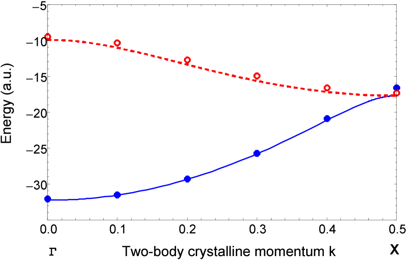
Figure 2: Many-body band structure of a periodic model system with two electrons in the triplet state obtained with SHDMC (dots) and compared with CI (lines). The figure shows the energy of the ground state and the first excited state as a function of the global crystalline momentum ${\bf k}$ (i.e., the many-body Bloch phase or twist angle).

IV Ground and excited states with applied magnetic field

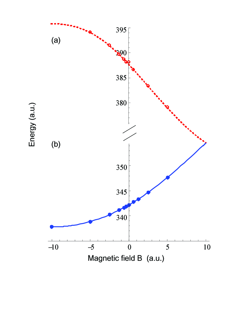
Figure 3: SHDMC results (dots) obtained for (a) the first excited state and (b) the ground state of a model system compared with CI results (lines) as a function of the magnetic field. The system consists of two electrons in a two-dimensional square in the triplet state. The results shown correspond to the ground and first excited states with $E$ symmetry that transform as $x+{\bf i}y$. The solution that transforms as $x-{\bf i}y$ can be obtained by changing the sign of $B$.

This section describes the results obtained with the generalization of SHDMC (described in Section II) for the ground and the first excited state of a model system with an applied magnetic field. The results are compared with CI calculations in the same model used in Refs. rosetta, ; keystone, and rockandroll, .

IV.1 Model system with magnetic field

Briefly, the lower energy eigenstates are found for two spinless electrons moving in a two-dimensional square with a side length $1$ and a repulsive interaction potential of the form $V({\bf r},{\bf r^{\prime}})=8\pi^{2}\gamma\cos{[\alpha\pi(x-x^{\prime})]}\cos{[\alpha\pi(y-y^{\prime})]}$ with $\alpha=1/\pi$ and $\gamma=4$. The many-body wave function is expanded in functions $\Phi_{n}({\bf R})$ that are eigenstates of the noninteracting system. The basis functions in $\{\Phi_{n}({\bf R})\}$ are linear combinations of functions of the form $\prod_{\nu}\sin(m_{\nu}\pi x_{\nu})$ with $m_{\nu}\leq 7$. Converged CI calculations were performed to obtain a nearly exact expression of the lower energy states of the system $\Psi_{n}({\bf R})=\sum_{m}a_{m}^{n}\Phi_{m}({\bf R})$. The matrix elements involving the magnetic vector potential ${\bf A}$ (in the symmetric gauge) were calculated analytically using the symbolic program Mathematica and were included in the CI Hamiltonian. The Jastrow factor was set to zero in the SHDMC run to facilitate a direct comparison between CI and SHDMC results.

This paper reports results for the triplet case. In the absence of a magnetic field, the triplet ground state is degenerate. Its orbital symmetry corresponds to the E symmetry of the D₄ group. One of the solutions with E symmetry transforms as $x$ and the other as $y$. Under an applied magnetic field, the time reversal symmetry is broken, and the $x$ and $y$ solutions are mixed. Under a magnetic field, the ground state can be expanded in a basis of functions that transform as $x\pm{\bf i}y$. The energy of the $x-{\bf i}y$ solution can be obtained from the energy of $x+{\bf i}y$ by changing $B$ to $-B$.

IV.2 Results and discussion

Figure 3 shows energies of the ground state and first excited state of the model system as a function of the magnitude of the magnetic field $B$ (the curl of the vector potential ${\bf A}$). The calculations were run using $\delta\tau=0.00004$ and $\tau=0.002$ and a total number of DMC steps of $10^{5}$ for each calculated point. The calculation for the ground state started from the noninteracting ground-state solution as a trial wave function. The result obtained for $B=0$ for the ground and first excited states compared well with the ones obtained with the same Hamiltonian in the triplet case reported fn:errorCI in Table I of Ref. rockandroll, . Note that in this case, the wave function is complex and the coefficients have the freedom to be complex. Thus, in contrast with Ref. rockandroll, , where a real wave function was enforced, here the phase was found within statistical error.

For $B\neq 0$, the time reversal symmetry is broken and so is the degeneracy of the $x\pm{\bf i}y$ solutions. For higher (lower) magnetic fields, the calculation began by using as the initial trial wave function the one obtained previously with a lower (higher) magnetic field.

The excited states were obtained using the method outlined in subsection II.3 and described in detail in Ref. rockandroll, . The lines show the CI results for reference. The calculation for the first excited state with $B=0$ started from a linear combination of the ground and first excited state of the noninteracting system orthogonal to the interacting ground state calculated earlier. The initial trial wave functions of the excited states for $B\neq 0$ were taken from the previous calculations with smaller $|B|$ (keeping the wave function orthogonal to the lower energy states with the operator $\hat{P}$). Clearly, Fig. 3b shows good agreement between SHDMC and CI results for the first excited state.

Table 1 summarizes the values obtained to construct Fig. 3. There is an excellent agreement in the calculations obtained for the ground state using SHDMC and CI. The SHDMC energy values are, within error bars converged FPDMC results indicating that the remaining convergence errors in the basis are small. The agreement is less satisfactory for the excited states than in the ground state (using the same computational time). It its clear that the residual projections are much larger for the excited state than for the ground.

An independent way to measure the quality of the wave function is the logarithm of the variance of the modulus of the weights given by

$$L_{var}=\ln{\sqrt{\frac{1}{N_{c}}\sum_{i,j}(|W_{i}^{kj}(k)|-1)^{2}}}\;.$$ (40)

The variance of the weights does not deteriorate as much as the residual projection for excited states, which might signal that the differences in the wave functions originate because CI and SHDMC minimize different things using a truncated basis. rockandroll

Table 1: Comparison of the excitation energies obtained for the ground and the first excited state of a model system with two spinless electrons and an applied magnetic field (see Fig. 3). $L_{rp}$ quantifies the overlap of the wave functions obtained with CI and SHDMC [see Eq. (39)]. $L_{var}$ is the variance of the modulus of the walkers‘ weights [see Eq. (40)].

—Ground State—

$B$	$E_{0}$ (SHDMC)	$E_{0}$ FPDMX	$E_{0}$ (CI)	$L^{0}_{rp}$	$L_{var}$
-3.2 $\pi$	337.823 (13)	337.820(7)	337.821	-9.9	-4.7
-1.6 $\pi$	338.877 (4)	338.867(4)	338.870	-12.7	-5.3
-0.8 $\pi$	340.261 (7)	340.256(5)	340.256	-12.9	-5.7
-0.4 $\pi$	341.143 (6)	341.153(5)	341.162	-10.3	-5.9
-0.2 $\pi$	341.646 (11)	341.662(6)	341.667	-13.6	-6.0
-0.1 $\pi$	341.931 (5)	341.930(7)	341.933	-14.2	-6.1
0.0 $\pi$	342.207 (7)	342.206(5)	342.208	-11.9	-6.1
0.2 $\pi$	342.771 (6)	342.782(6)	342.782	-12.4	-6.0
0.4 $\pi$	343.387 (5)	343.392(4)	343.390	-10.8	-6.0
0.8 $\pi$	344.696 (8)	344.689(6)	344.704	-11.7	-5.8
1.6 $\pi$	347.699 (8)	347.684(5)	347.697	-9.4	-5.2

—First Excited State— $B$ $E_{1}$ (SHDMC) $E_{1}$ (CI) $L^{1}_{rp}$ $L_{var}$ -1.6 $\pi$ 394.161 (19) 394.114 -7.4 -5.0 -0.8 $\pi$ 391.532 (12) 391.504 -7.9 -5.4 -0.4 $\pi$ 389.744 (12) 389.741 -9.1 -5.7 -0.2 $\pi$ 388.786 (10) 388.769 -9.9 -5.8 -0.1 $\pi$ 388.253 (13) 388.265 -9.8 -5.7 0.0 $\pi$ 388.205 (44) 387.750 -5.7 -5.0 0.2 $\pi$ 386.697 (17) 386.694 -8.9 -5.7 0.8 $\pi$ 383.415 (14) 383.407 -8.9 -5.4 1.6 $\pi$ 379.159 (28) 379.057 -7.9 -4.8

V Test with Coulomb interactions

The calculations with Coulomb interactions were performed in the same system studied for the ground state in Ref. keystone, and for excited states in Ref. rockandroll, but now with the additional ingredient of an applied magnetic field. The more challenging triplet (antisymmetric) state was chosen for this study.

The calculations were run with the same parameters and basis as in Fig. 3 and Table 1 but with a Coulomb interaction potential of the form $V({\bf r},{\bf r^{\prime}})=20\pi^{2}/|{\bf r-r\prime}|$. Since the average of the Coulomb interaction is much larger than the single-particle energy differences, the system is in the highly correlated regime.

Table 2: SHDMC and FPDMC energies as a function of an applied magnetic field for a model system with two electrons in a triplet state in a square box with Coulomb interactions. The quality of the wave function is measured by $L_{var}$ [see Eq. (40)].

State	$B$	SHDMC	PFDMC	$L_{var}$
0	-1.60 $\pi$	401.65 (2)	401.67(4)	-4.1
0	-1.26 $\pi$	401.80 (3)		-4.2
0	-0.80 $\pi$	401.92 (3)	401.87(4)	-4.2
0	-0.40 $\pi$	403.50 (6)	402.39(7)	-3.4
0	-0.20 $\pi$	402.97 (4)	402.60(5)	-4.1
0	0.00	402.76 (4)	402.58(3)	-4.0
0	0.40 $\pi$	403.23 (2)	403.20(3)	-4.6
0	0.80 $\pi$	403.87 (3)	403.73(3)	-4.2
0	1.26 $\pi$	404.93 (6)		-3.7
0	1.60 $\pi$	405.54 (9)	405.16(4)	-3.8
1	-0.40 $\pi$	465.37 (10)		-3.0
1	-0.20 $\pi$	468.55 (7)		-3.5
1	0.00	454.39 (8)		-3.4
1	0.40 $\pi$	451.76 (8)		-3.2
2	-0.40 $\pi$	486.89 (7)		-3.2

Table 2 displays the values obtained for the model system with Coulomb interactions for the ground state and some excitations as a function of the magnetic field. The quality of the wave function is characterized by the logarithm of the variance of the modulus of weights given by Eq. (40). Note that the variance of the weights increased when Coulomb interactions are considered when compared with the case of the model interaction. This is due to the Coulomb singularity and the lack of a Jastrow factor. While the variance of the weights is larger in the Coulomb case, the quality of the wave function improves from one SHDMC recursive iteration to the next (see below).

V.1 Improvement of the wave function’s node and phase with SHDMC

Figure 4 shows the evolution of the real (a) and the imaginary (b) parts of the local energy $E_{L}({\bf R})$ as a function of the DMC step for the first excited state of two electrons in a square box with an applied magnetic field of $0.4\pi$. The calculations started with a trial wave function with two nonzero coefficients chosen to be orthogonal to the ground state calculated earlier. It can be clearly seen in Fig. 4(a) that as the SHDMC algorithm progresses, the real part of the local energy is quickly reduced and stabilized at the first excited state energy. The imaginary part of the $E_{L}({\bf R})$ should be zero for an eigenstate; otherwise, the divergence of the current is nonzero ortiz93 . In SHDMC this strong condition is satisfied only as the number of recursive iterations, the number of configuration sampled $N_{c}$, and the size of the basis $N_{b}$ retained in the wave function tend to infinity. Figure 4(b), however, clearly shows that the variance of the raw data obtained for $Im[E_{L}({\bf R})]$ is reduced as the SHDMC algorithm progresses. This is a clear indication of improvement of the phase of the wave function.

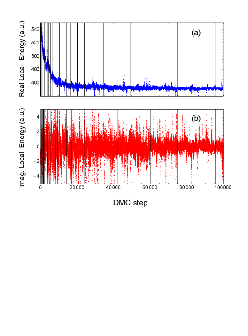
Figure 4: (Color online) (a) Average of the real part of $E_{L}({\bf R})$ obtained with 200 walkers as a function of the DMC step. The results correspond to the first excited state that transforms as $x+{\bf i}y$ with $E$ symmetry of the group $D_{4}$ of two electrons with Coulomb interactions in a square box with an applied magnetic field units $B=0.4\pi$. (b) Average of the imaginary part of $E_{L}({\bf R})$ as a function of the DMC step for the same case. The vertical lines mark the end of the SHDMC block when the wave function is updated.

Figure 5 shows the evolution of logarithm of the variance of the weights [see Eq. (40)] as a function of the SHDMC block index (the number of wave function updates). The reduction in weight variance is a clear indication of convergence of the trial wave function towards an eigenstate of the Hamiltonian rockandroll .

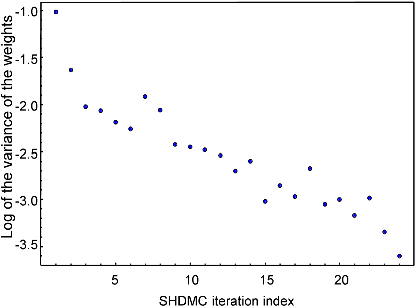
Figure 5: (Color online) Logarithm of the variance of the modulus of weights as a function of the SHDMC block index $\ell$. The results correspond to the first excited state with $B=0.4\pi$ and Coulomb interactions (the run shown in Fig. 4).

VI Summary and perspectives

A method that allows the calculation of the complex amplitude of a many-body wave function has been presented and validated with model calculations. An algorithm that finds the complex wave function is essential for any study of many-body Hamiltonians with periodic boundary conditions or under external magnetic fields. The method converges to nearly analytical results obtained for model systems under applied magnetic fields or periodic boundary conditions, with an accuracy limited only by statistics and the flexibility of the wave function sampled.

It is found that for some eigenstates, the ones where the phase is a scalar function of ${\bf R}$, there is a special gauge transformation in which wave function is real. For this class of eigenstates the original proof of convergence of SHDMC applies. For complex wave functions some fermionic eigenstates may not have nodes. In the latter case, as in the case of bosonsrockandroll ; reatto82 , the convergence of SHDMC is not affected since the wave function can evolve everywhere.

This new approach goes beyond both fixed-phase DMC ortiz93 and SHDMC keystone ; rockandroll ; rollingstones . As in the real wave function version of SHDMC, the method is recursive and the propagation to infinite imaginary time is achieved as the number of iterations increases. As in FPDMC, the walkers evolve under an effective potential that incorporates the gradient of the phase of the trial wave function and the vector potential of the magnetic field. But in this new algorithm, in contrast to FPDMC, the complex amplitude of the wave function is free to adjust both its modulus and its phase. After each iteration, the trial wave function is improved following a short time evolution of an ensemble of walkers. These walkers follow the equation of motion of a generalized importance sampling approach. Unlike previous attempts, the walkers carry a complex weight resulting from eliminating the fixed-phase constraint in the time evolution of the mixed probability density. The modulus of the weight can be used to calculate real observables, such as the energy. The phase of the weight of the walkers is used to improve the phase of the trial wave function in the following iteration. As in earlier versions of SHDMC, the modulus of the weights is also used to improve, simultaneously, the node if there is any and the phase of the trial wave function.

This free amplitude SHDMC method can be used to calculate not only the ground state but also low energy excitations rockandroll within a DMC context. Comparisons with nearly analytical results in model systems demonstrate that the new approach converges to the many-body wave function of systems with applied magnetic fields or with periodic boundary conditions for low energy excitations.

This recursive method finds a solution to “the phase problem” and, if there is any, finds the node at the same time. The many-body wave function can be used, in principle, to calculate any observable. However, in very large systems, when convergence with the size of the wave function basis cannot be fully achieved, a standard fixed-phase calculation should be performed as a final step to obtain a more accurate energy.

Scaling and cost: An analysis of the minimum cost required to determine the node and the phase has to take into account the number of independent degrees of freedom of the Hilbert space. Arguably, no method could scale better than linear in the number of independent degrees of freedom of the problem studied; otherwise, some degrees of freedom would be dependent from each other. A real-space expansion of the many-body wave function with fixed resolution $L_{R}$ is ideal for counting independent degrees of freedom. The resolution $L_{R}$ can be connected to the energy cutoff of the excitations in a multideterminant expansion. For a complex wave function, each point in the many-body space ${\bf R}$ has two independent degrees of freedom (modulus and phase). If the volume of a system is proportional to the number of electrons $N_{e}$, its size scales as $L\approx\alpha N_{e}^{1/3}$ (where $\alpha$ is of the order of the Bohr radius $a_{B}$). Taking into account the $N_{e}!$ permutations of identical particles, one finds $(L/L_{R})^{3N_{e}}/N_{e}!$ independent degrees of freedom for each spin channel to determine the phase $\phi({\bf R})$. Thus, the number of independent degrees of freedom scales as $\exp\{N_{e}(3\log(\alpha/L_{R}))+1)\}$. The node $S_{T}({\bf R})$, if there is any, requires one less dimension (which, if the nodal surface is not too convoluted, could reduce the number of degrees of freedom by only up to a factor $(L/L_{R})$). Since the number of independent degrees of freedom of the phase increases exponentially with $N_{e}$, for a fixed resolution $L_{R}$ one cannot find the phase with an algorithm polynomial in $N_{e}$.

This generalization of the SHDMC method, though tested in small systems, is targeted to be used in large systems. The numerical cost of SHDMC scales linearly with the number of independent degrees of freedom of the phase per recursive step. However, the number of independent degrees of freedom (i.e, the size of the basis expansion) should increase exponentially with the number of electrons $N_{e}$ for a fixed resolution. The accuracy of SHDMC is limited by the size of the basis sampled, the statistical error, and the number of recursive iterations. The number of recursive steps required increases if the product between $\tau$ and the lowest energy excitations is small. The SHDMC method can be used in combination with other optimization approaches to accelerate convergence in that limit.

The scaling of the cost of exact diagonalization methods such as CI is at least quadratic with the number of degrees of freedom. Often a CI calculation is used to preselect a multideterminant expansion to be improved within a VMC context before a final FPDMC run. An advantage of SHDMC is that it incorporates the Jastrow in the sampling of the coefficients. Thus SHDMC might be more efficient than a CI filtering for large systems. The linear scaling of SHDMC suggests that it could be the method of choice to optimize the wave function phase and nodes for calculations in periodic solids.

The optimization of many-body wave functions with current in periodic boundary conditions is now possible. Therefore, the new method can be used as a tool to perform transport calculations including many-body effects. The calculation of systems with an applied magnetic field is challenging, even in the case of small molecules and atoms and particularly so when the magnetic field, the many-body interactions, and the kinetic energy are of the same order of magnitude jones96 . The calculations reported in this paper, though in a simple model, suggest that the method can be applied to the study of molecular or atomic systems in that difficult regime.

Our recent successful application of the ground-state algorithm for real wave functions keystone to molecular systems rollingstones supports the idea that this generalization of SHDMC can also be useful for real ab-initio calculations beyond model systems. The implementation of the algorithm in state-of-the-art DMC codes has been done. Initial results in atomic systems show that the many-body wave function improves, which is shown by a reduction of the average local energy, the energy variance and the variance of the imaginary contribution to the total energy.

- (1) P. Hohenberg and W. Kohn, Phys. Rev. 136, B864 (1964).
- (2) J. B. Anderson, Int. J. Quantum Chem. 15, 109 (1979).
- (3) P. J. Reynolds, D. M. Ceperley, B. J. Alder, and W. A. Lester, J. Chem. Phys. 77, 5593 (1982).
- (4) B. L. Hammond, W. A. Lester, Jr., and P. J. Reynolds, Monte Carlo Methods in Ab Initio Quantum Chemistry (World Scientific, Singapore-New Jersey-London-Hong Kong, 1994).
- (5) D. M. Ceperley and B. J. Alder, Phys. Rev. Lett. 45, 566 (1980).
- (6) G. Ortiz, D. M. Ceperley, and R. M. Martin, Phys Rev. Lett. 71, 2777 (1993).
- (7) A. J. Williamson, R. Q. Hood, and J. C. Grossman, Phys. Rev. Lett. 87, 246406 (2001).
- (8) D. Alfe and M. J. Gillan, Phys. Rev. B 70, 161101(R) (2004).
- (9) F. A. Reboredo and A. J. Williamson, Phys. Rev. B 71, 121105(R) (2005).
- (10) D. M. Ceperley, J. Stat. Phys. 63, 1237 (1991).
- (11) M. Troyer and U. J. Wiese, Phys. Rev. Lett. 94, 170201 (2005).
- (12) W. M. C. Foulkes, L. Mitas, R. J. Needs, and G. Rajagopal, Rev. Mod. Phys. 73, 33 (2001).
- (13) G. Ortiz, and D. M. Ceperley Phys. Rev. Lett. 75, 4642 (1995).
- (14) M. D. Jones, G. Ortiz, and D. M. Ceperley, Phys. Rev. E, 55, 6202, (1997).
- (15) A. D. Güçlü and C. J. Umrigar, Phys. Rev. B, 72, 045309 (2005); A. D. Güçlü, G. S.. Jeon, C. J. Umrigar and J. K. Jain, Phys. Rev. B 72, 205327 (2005); G. S. Jeon, A. D. Güçlü, C. J. Umrigar, and J. K. Jain, Phys. Rev. B 72, 245312, (2005).
- (16) C. J. Umrigar, J. Toulouse, C. Filippi, S. Sorella, and R. G. Hennig, Phys. Rev. Lett. 98, 110201 (2007).
- (17) A. Lüchow, et al., J. Chem. Phys. 126, 144110 (2007).
- (18) F. A. Reboredo, R. Q. Hood, and P. R. C. Kent, Phys. Rev. B 79, 195117 (2009).
- (19) F. A. Reboredo, Phys. Rev. B 80, 125110 (2009).
- (20) M. Bajdich, M. L. Tiago, R. Q. Hood, P. R. C. Kent, and F. A. Reboredo, Phys. Rev. Lett. 104, 193001 (2010).
- (21) is not obtained; the new is sampled directly.
- (22) F. A. Reboredo and P. R. C. Kent, Phys. Rev. B 77, 245110 (2008).
- (23) A complex energy reference stabilizes the run for arbitrary gauge choices for the vector potential .
- (24) Equation (2) in OCM work is only strictly valid if , otherwise it is the so-called fixed-phase approximation ortiz93 .
- (25) A complete basis in the symmetric space can be used to calculate bosons. Other symmetries of the wave function can be enforced with the selection of the basis rockandroll .
- (26) Since is essentially an iteration index, it is omitted in the trial wave function phase and amplitude for clarity.
- (27) C. J. Umrigar, M. P. Nightingale, and K. J. Runge, J. Chem. Phys. 99, 2865 (1993).
- (28) C. Umrigar (private communication).
- (29) L. Reatto, Phys. Rev. B 26, 130 (1982).
- (30) The position of the cut in the complex plane of the Riemann surface into sheets is arbitrary. Therefore, the discontinuities in the gradient and the effective potential are no physical if they can be removed changing .
- (31) J. D. Jackson, Classical Electrodynamics third edition (John Willey & Sons, Inc) New York, (1998).
- (32) D. M. Ceperley and B. Bernu, J. Chem. Phys. 89, 6316 (1988); B. Bernu, D. M. Ceperley, and W. A. Lester, Jr., J. Chem. Phys. 93, 552 (1990).
- (33) W. Purwanto, S. Zhang, and H. Krakauer, J. Chem. Phys. 130, 094107 (2009).
- (34) K. Hoffman and R. Kunze, Linear Algebra second edition (Prentice -Hall) New Jersey (1971).
- (35) E. Prugovec̆ki Quantum Mechanics in Hilbert Space (Academic Press) New York (1981).
- (36) N. W. Ashcroft and N. D. Mermin, Solid State Physics (Saunders College Publishing Harcourt Brace College Publishers, 1976).
- (37) G. Rajagopal, R. J. Needs, A. James, S. D. Kenny, and W. M. C. Foulkes, Phys. Rev B 51, 10591 (1995).
- (38) R. Krc̆már, A. Gendiar, M. Mos̆ko, R. Németh, P. Vagner, L. Mitas Physica E 40,1507 (2008).
- (39) C. Lin, F. H. Zong, and D. M. Ceperley, Phys. Rev. E 64, 016702 (2001).
- (40) The term “twist angle” was introduced tbc to avoid confusion with other usages of the term “phase”. Here the term “many-body Bloch phase” is also mentioned since the Bloch theory is well understood outside the many-body field.
- (41) L.K. Wagner, M. Bajdich, and L. Mitas, J. Comp. Phys. 228, 3390 (2009).
- (42) M. D. Jones, G. Ortiz, and D. M. Ceperley, Phys Rev. A 59, 2875 (1999).
- (43) F. A. Reboredo, M. Bajdich and P. R. C. Kent (work in progrees).
- (44) The energy unit is and the magnetic unit is given by .
- (45) There was a small error in the CI calculations reported in Ref. rockandroll, .
- (46) M. D. Jones, G. Ortiz, and D. M. Ceperley, Phys Rev. A 54, 219 (1996).