Catastrophic regime shifts in model ecological communities are true phase transitions

Abstract

Ecosystems often undergo abrupt regime shifts in response to gradual external changes. These shifts are theoretically understood as a regime switch between alternative stable states of the ecosystem dynamical response to smooth changes in external conditions. Usual models introduce nonlinearities in the macroscopic dynamics of the ecosystem that lead to different stable attractors among which the shift takes place. Here we propose an alternative explanation of catastrophic regime shifts based on a recent model that pictures ecological communities as systems in continuous fluctuation, according to certain transition probabilities, between different micro-states in the phase space of viable communities. We introduce a spontaneous extinction rate that accounts for gradual changes in external conditions, and upon variations on this control parameter the system undergoes a regime shift with similar features to those previously reported. Under our microscopic viewpoint we recover the main results obtained in previous theoretical and empirical work (anomalous variance, hysteresis cycles, trophic cascades). The model predicts a gradual loss of species in trophic levels from bottom to top near the transition. But more importantly, the spectral analysis of the transition probability matrix allows us to rigorously establish that we are observing the fingerprints, in a finite size system, of a true phase transition driven by background extinctions.

1 Introduction

Ecosystems are exposed to continuous changes in external conditions. Seasonal changes of environmental conditions, climate oscillations, variations in the amount of resources and nutrient loading, habitat fragmentation, harvest or loss of species diversity are a few examples of these gradual changes. They often change slowly, even linearly, with time [1]. It is usually assumed that the response of the system to external changes is smooth most of the times. However, occasionally sudden changes can occur. For example, the sudden loss of transparency and vegetation observed in shallow lakes due to human-induced effects [2]; corals overgrown by macro-algae in the Caribbean reef seem to shift between two stable states rather than responding smoothly to external conditions [3, 4]; or in savannahs, sparse trees with a grass layer can switch to a dense woody state as a result of the alternation in fire and grazing regimes [5, 6]. All these phenomena share the feature that ecosystems seem to change between two different stable states. Sudden changes between two regimes are the so-called catastrophic shifts [7]. Hence, when subjected to a slowly changing external control variable, ecological communities may show little change until a critical point is reached. Then a sudden switch to a contrasting state can occur.

The simplest theoretical explanation to catastrophic regime shifts comes from the existence of alternative stable states in the dynamical ecosystem response to gradual changes. The shift between two alternative stable states is responsible for the transition. Often the existence of different stable states is associated to nonlinearities. A non-linear ecosystem response to smooth external variations allows for the existence of alternative stable states [7, 8]. The effects of nonlinearities have also been observed in natural communities. For example, it has been established that the non-linear dynamics of overexploited marine ecosystems magnifies the variability in the abundance of exploited species [9, 10].

In these models, ecosystems are described from a macroscopic viewpoint. Usually a global magnitude, representative of the whole community, is used as fundamental variable (for instance, the total biomass density). Models are basically devised to describe the time evolution of this magnitude by means of non-linear functional responses [7, 11]. Recently this paradigm has been applied to spatially extended interacting communities [12, 13]. This theoretical approach is conceptually very similar to the traditional thermodynamic explanation of phase transitions in physical systems, such as the liquid-vapor transition. The lack of convexity of theoretical thermodynamic potentials —such as free energy— leads to alternative stable states corresponding to liquid and vapor and both phases coexist below a certain critical temperature. In [11, 12, 13] the analogy is very clear. The dynamics of biomass density follows a logistic growth with carrying capacity $K$ and a density-dependent consumption term modelled as a sigmoidal (Holling’s type III) functional response. It is precisely this type of functional response which allows for the existence of two separate, stable equilibrium points in the dynamics above a certain critical value of the carrying capacity.

However, the current understanding of phase transitions in physical systems goes beyond phenomenological, macroscopic models. The microscopic approach of Statistical Mechanics represents a more fundamental way of understanding phase transitions, and many elaborated theories have been developed to account for abrupt shifts in physical systems. Our aim in this paper is to propose an alternative explanation, based mainly in a microscopic approach, to these catastrophic regime shifts in ecosystems. In fact, we will show that a linear functional response in the dynamics of individual species can lead to a global shift in the ecosystem between a species-rich attractor and a state with low species richness. The early-warnings that are usually mentioned as precursors of catastrophic regimes, like the increasing fluctuations near the transition [9, 14] or the appearance of trophic cascades [15], will be recovered within our framework.

Based on an assembly model introduced recently [16, 17, 18], that pictures ecosystems as complex, stable entities which keep on fluctuating between different micro-states through successional invasions of rare species, we will introduce a background species extinction rate accounting for the gradual, external variations to which natural communities are subjected. We will find a threshold rate above which the system undergoes a phase transition, and the rate will play the role of the shift control parameter. We will show that fluctuations become critical in the vicinity of the transition, and that the ultimate collapse of the ecosystem correspond to a gradual loss of species from bottom to top. It is worth remarking that trophic cascades have been recognized as signals of overexploitation in marine communities [15].

The main feature of the assembly model presented in [16] is to provide a complete characterization of the phase space of the system. The time evolution of the system is fully described by means of a Markov chain. Under the effect of increased spontaneous extinctions, an initially species-rich ecosystem can move to a region of the phase space where the species richness decreases. Through a spectral analysis of the transition probability matrix we will be able to show rigorously that the shift we observe corresponds to the “trace” of a true phase transition —according to the definition of Statistical Mechanics— in finite size.

The paper is organized as follows. In Section 2 we will review the main features of the assembly model and discuss the effect of a background species extinction rate in the ecosystem. We will find that the Markov process is ergodic and that there is an increasing probability of finding the ecosystem close to extinction as the rate grows. In Section 3 we will study some signals with anomalous behavior near the shift, and show under which conditions hysteresis in the average number of species arise. In Section 4 we will show that the observed behavior would correspond to a true phase transition were the system infinitely large. So we can conclude that what we are actually observing are the fingerprints of this transition in systems of finite size.

2 Background species extinction

Our starting point is a simple assembly model that we have recently introduced [16]. Let us briefly summarize its main features. We describe ecological communities introducing three basic simplifications. First, species are arranged in a finite number of trophic levels, and feeding relationships take place exclusively between contiguous trophic levels. Second, the strength of interactions is averaged over the whole community (mean-field), thus all species at the same level are trophically equivalent. And third, population dynamics is modelled by Lotka-Volterra equations. In spite of these oversimplifications, the resulting communities reproduce all results previously found in earlier assembly models [16, 19, 20].

The mean-field assumption allows us to represent each community by the set of occupancy numbers of each trophic level, $\{s_{\ell}\}_{\ell=1}^{L}$, $L$ being the total number of levels and $s_{\ell}$ the number of species at level $\ell$. All species are considered as consumers, with uniform intrinsic average mortality rate $\alpha$. Predation between adjacent levels is modelled by constants $\gamma_{+}$ and $\gamma_{-}$. The former represents the per-capita rate of increase in population due to feeding, the latter accounts for the mean damage caused by being predated. Communities are sustained by a primary, abiotic resource characterized by its intrinsic growth rate $R$. This represents the saturation value that the resource reaches at equilibrium in absence of predation, and measures the energy influx available for each community. Species at the first trophic level predate on this resource and transfer the energy upwards in the food web. Increasing $R$ has the effect of allowing more trophic levels and more species in each level as well (see [16]).

Population dynamics is ruled by Lotka-Volterra equations, which guarantees the existence of a unique interior equilibrium point. Equilibrium communities whose populations are above of a given extinction threshold $n_{c}$ are considered as viable. For a full account on the population dynamics and the implications of the invasion dynamics in this model, we refer the reader to [17].

Our model represents a substantial improvement with respect to former assembly models in that it provides a complete characterization of all possible invasion pathways within the set of viable communities. Equivalently, an assembly graph $\mathcal{G}$, i.e. the graph whose nodes are viable communities and whose links connect communities through invasions, can be fully obtained under these assumptions. The existence of a extinction threshold renders this graph finite. We assigned to each link a certain transition probability dependent on an invasion rate $\xi$. The mean time between consecutive invasions, $\xi^{-1}$, is assumed to be large compared to the time that each community needs to restore its dynamical equilibrium.

Weighting the links of $\mathcal{G}$ with probabilities defines a finite Markov chain over the set of viable communities. In [18] we showed that this chain is aperiodic, hence communities can be either transient or recurrent. We always found a single connected set of recurrent communities upon increasing the resource saturation $R$. This set was either a single absorbing community or a more complex end state of recurrent communities, the Markov process being ergodic over those complex sets. The existence of complex end states is probably one of the most remarkable results of the model (for a detailed account of results see [18]).

According to this picture, ecosystems evolve though successional invasions until reaching a final end state, either a single absorbent community or a complex, closed set of recurrent communities. When the process reaches a complex end state, successional invasions transform the ecosystem into some other of the communities belonging to that set, so the process visits all communities in this set, albeit with different frequencies —given by the asymptotic probability distribution of the Markov process within this set. In terms of species this means that communities keep continuously changing and eventually, after enough time has elapsed, all the original species in the ecosystem will be replaced by new ones. Therefore the ecosystem keeps on fluctuating between the different communities comprising the closed set, which persists as a robust, stable entity.

Let us now introduce a rate of spontaneous extinctions. Species in natural communities are often subject to overexploitation. Intensive hunting in terrestrial communities or the increasing fishing pressure in marine ecosystems are good examples of this. Sometimes the species population is seriously altered due to habitat destruction, in other cases due to exposure to epidemics or diseases. Many effects like these ones can effectively decrease to critical levels the number of individuals of a certain species or even cause its extinction. We will represent these situations by means of a probability rate, $\eta$, which accounts for the probability per unit time for a species to go extinct for reasons other than being eaten. Actually this probability rate should depend on the species and its environment but, for the sake of simplicity, we will assume it uniform for all species.

Our model is amenable to introduce background extinctions in a simple way. Elementary processes in the original model for $\eta=0$ were transitions between viable communities carried out by single-species invasions. Now two different processes, either invasion or extinction, can connect two communities. Thus, for a given community $E$ with $L$ trophic levels, we need to determine all the possible transitions carried out by invasions and spontaneous extinctions at each level (and by invasions at level $L+1$ as well). The graph $\mathcal{G}$ will now contain both types of transitions. The links corresponding to extinction transitions can be obtained just as the invasion ones [16]. Given a community $E\in\mathcal{G}$, we randomly remove one of its species and calculate the equilibrium population densities of the resulting community $E^{\prime}$. If the community is viable, then we establish a transition between $E$ and $E^{\prime}$. If some species go below the extinction level $n_{c}$, then we apply the same sequential extinction procedure that was followed to obtain the invasion graph (for a detailed discussion of this procedure see [17]). We repeat these sequential extinctions until the final community $E^{\prime\prime}$ is viable.

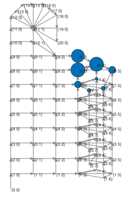
(a)              (b)

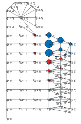
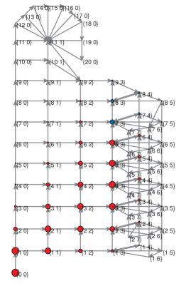
(c)              (d)

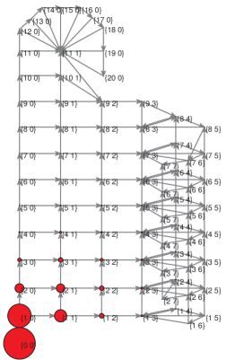
Figure 1: Assembly graph $\mathcal{G}$ obtained for $R=120$, comprising 79 communities with up to 2 trophic levels, for 4 increasing values of $\eta/\xi$. Diameter of nodes is proportional to their asymptotic probability. Labels of nodes represent species occupancies $\{s_{1},s_{2}\}$. For the sake of clarity, only transitions carried out through invasions are shown. For $\eta=0$, the recurrent set contains 9 nodes (colored in blue). Red nodes represent transient states for $\eta=0$. (a) The most probable communities are those in the recurrent set ($\eta/\xi=0.05$). (b) Some communities, close to this set, are visited with high frequency ($\eta/\xi=0.3$). (c) Almost none of the 9 originally recurrent communities are visited ($\eta/\xi=0.6$). (d) The most probable community corresponds to the total extinction state ($\eta/\xi=1$).

The transition probability $p_{ij}$ for the transition from community $i$ to community $j$ can be written as

$$p_{ij}=\delta_{ij}+\xi q_{ij}+\eta u_{ij},$$ (1)

where $\delta_{ij}$ is the Kronecker delta, and matrices $Q=(q_{ij})$ and $U=(u_{ij})$ account for the relative frequency of invasions and extinctions, respectively. For $i\neq j$ we set $q_{ij}=n_{ij}/(L+1)$, $n_{ij}$ being the number of different invasions of $i$ that lead to $j$ and $L+1$ the total number of possible invasions of $i$, provided it has $L$ trophic levels. For $i\neq j$ we define $u_{ij}=m_{ij}/S_{i}$, where $m_{ij}$ is the number of different extinctions in $i$ that lead to $j$ and $S_{i}=\sum_{\ell=1}^{L}s_{\ell}^{(i)}$ is the number of possible extinctions of $i$. We set $u_{ii}=0$ and calculate the diagonal of $Q$ so that $P=(p_{ij})$ is a stochastic matrix. This yields

$$q_{ii}=-\sum_{i\neq j}\left(q_{ij}+\frac{\eta}{\xi}u_{ij}\right).$$ (2)

When $\eta=0$ we recover the original transition matrix of our model (see [18]). This is quite a singular case, though, not representative of what happens for any $\eta>0$ —no matter how small.

In fact, there is a major difference between the cases $\eta=0$ and $\eta>0$, regarding the properties of the Markov chain. For any $\eta>0$, there is a non-zero probability for all the $S$ species in a community to go extinct. Let $\Delta t$ be the time unit between consecutive iterations of the Markov chain. Thus the removal of all species caused by sequential spontaneous extinctions has a probability at least equal to $(\eta\Delta t)^{S}$. The non-vanishing probability of total extinction implies that the process can return to the initial state (the empty community $\varnothing$) and therefore the Markov chain becomes ergodic. This has to be compared with the former model ($\eta=0$), for which we just found a tiny fraction of recurrent states, and almost all the communities in the assembly graph were transient [16, 18].

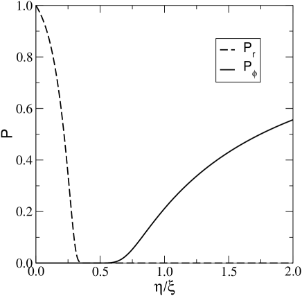
Figure 2: Probability $P_{\rm r}$ of finding the process in one of the communities of the recurrent set for $\eta=0$ (dashed line), and probability $P_{\varnothing}$ of the empty community (full line), as functions of the ratio $\eta/\xi$, for $R=1340$.

Ergodicity implies that any possible state of the ecosystem can be reached with a non-zero —albeit sometimes small— asymptotic probability. According to (1) we simply need to solve the linear system

$$0=\pi\left(Q+\frac{\eta}{\xi}U\right)$$ (3)

to obtain the (row) vector $\pi$ of asymptotic probabilities $\pi_{i}$ for all $i\in\mathcal{G}$. Therefore the asymptotic distribution depends on the relative strength between rates. We expect that, when this ratio is small enough, the subset of communities with the highest probability coincides with the recurrent subset found for $\eta=0$. However, as this ratio increases, the probability of finding the process within this subset should decrease. This effect can be observed in Figure 1, where we plot $\mathcal{G}$ with its asymptotic distribution for $R=120$ and 4 values of the quotient $\eta/\xi$. The remaining parameters of the model have been set as in our previous work: $\alpha=1$, $\gamma_{+}=0.5$, $\gamma_{-}=5$, $\rho=0.3$ and $n_{c}=1$. (We will use this set of parameters throughout this paper.) As $\eta/\xi$ increases, communities that were recurrent for $\eta=0$ are visited with decreasing asymptotic probabilities. Eventually, when the ratio is large enough, these communities are hardly visited and the process stays with high probability in communities close to the empty ecosystem, $\varnothing$.

This effect is more clearly seen in terms of the dependence of $P_{\rm r}$ —the probability of finding the process in any of the communities of the recurrent set for $\eta=0$— and $P_{\varnothing}$ —the probability of finding the ecosystem extinct— on $\eta/\xi$. A typical behavior of these probabilities is depicted in Figure 2. This plot corresponds to a resource saturation $R=1340$, for which $\mathcal{G}$ has 397698 nodes and 539 recurrent communities. In Figure 2 we can observe an abrupt decrease of $P_{\rm r}$ at $\eta/\xi\approx 0.33$, and $P_{\varnothing}$ increases abruptly as well when $\eta/\xi\approx 0.65$. Needless to say, these two magnitudes resemble the typical behavior of order parameters in the vicinity of a phase transition. A small increase in $\eta$ causes a shift from the stable, recurrent set at $\eta=0$ to communities close to extinction. In this sense, increasing background extinctions drive the system from a stable, species-rich attractor to a species-poor region of the phase space. The system thus undergoes a catastrophic regime shift analogous to those commonly observed in overexploited ecological communities [2]–[6].

3 Signals of catastrophic regime shifts

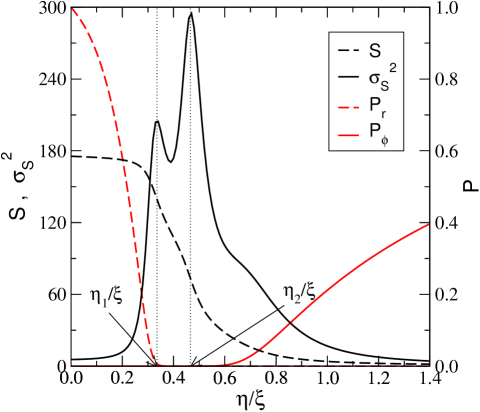
Figure 3: Average number of species (black dashed line) and its variance (black full line) as functions of $\eta/\xi$, for $R=1340$. The average number of species decreases monotonically whereas its variance exhibits a double peak at values $\eta_{1}/\xi\approx 0.33$ and $\eta_{2}/\xi\approx 0.46$. The first one coincides with the abrupt drop of $P_{\rm r}$ (red dashed line) but the second one precedes the increase of $P_{\varnothing}$ (red full line) announcing it.

From the perspective of conservation and management of ecosystems, it is very important to determine some signals that may alert of the proximity of a catastrophic transition. These are the so-called early-warnings of catastrophic regime shifts [14], and act as flags for the approach of a critical threshold. Although our model is minimalistic, the phenomenology of several magnitudes reveal a critical behavior near the shift described in the previous section. Now, upon gradually increasing the external “stress” (i.e., the ratio $\eta/\xi$) on our system, we will observe abrupt changes in these magnitudes close to the regime shift.

We shall begin assuming very slow variations in $\eta/\xi$, i.e., the ecosystem undergoes very many invasions before changes in the control parameter are noticeable. In this situation we can assume that the community is always at is steady state. At the end of this section we will analyze the effect of relaxing this assumption and allowing for a mixing of these two time-scales: the scale of variation of the stress and the scale of invasion.

A first precursor of the shift is the fluctuation of the mean number of species in the ecosystem. In [12] fluctuations were measured by the spatial heterogeneity of a single magnitude (a biomass density) representing the community as a whole, whereas the kind of fluctuations we are considering here are due to changes in the average number of species induced by invasions and spontaneous extinctions. In Figure 3 we plot the average number of species $S=\sum_{i\in\mathcal{G}}\pi_{i}S_{i}$, where $S_{i}$ is the total species richness of the $i$-th community. Its fluctuations are measured by the variance

$$\sigma_{S}^{2}=\sum_{i\in\mathcal{G}}\pi_{i}S_{i}^{2}-S^{2}.$$ (4)

The rapid growth of fluctuations provides an alert of the proximity of the catastrophic shift [7, 12, 14] Fluctuations for $R=1340$ exhibit a double peak at $\eta_{1}\approx 0.33\xi$ and $\eta_{2}\approx 0.46\xi$. The first one is related to the abrupt drop of the probability $P_{\rm r}$ that we showed in Section 2. In addition, these two peaks correspond to a gradual decrease in the number of species at each trophic level, as we will show below.

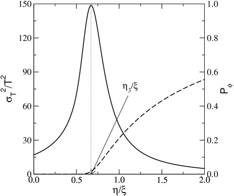
Figure 4: Relative variance $\sigma_{T}^{2}/T^{2}$ of the first-return time (average $T=P_{\varnothing}^{-1}$) to the empty ecosystem (full line), compared to the probability of total extinction $P_{\varnothing}$ (dashed line), for $R=1340$. The maximum of the relative variance roughly coincides with the point at which $P_{\varnothing}$ starts to increase. This maximum is reached at $\eta_{3}/\xi\approx 0.67$.

The second peak at $\eta_{2}/\xi$ announces the abrupt increase of $P_{\varnothing}$, but does not coincides with it. The increase of this probability is connected to the fluctuations of the time of first return to the empty community, whose mean value is given by $T=P_{\varnothing}^{-1}$. Using the first-passage distribution of the Markov chain [21], we can calculate the relative variance $\sigma_{T}^{2}/T^{2}$ (see Appendix for details) and the result is shown in Figure 4. The maximum relative fluctuation occurs nearly at the onset of increase of $P_{\varnothing}$, $\eta_{3}\approx 0.67\xi$. We thus expect that relative fluctuations in the average return time to any state $i$ close to $\varnothing$ will be amplified close to the extinction transition. This notwithstanding, it is hard to figure out how this fluctuation could be used in practice as a signal of the catastrophe.

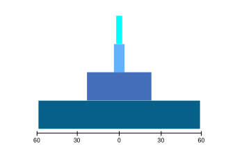
(a)     (b)

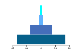
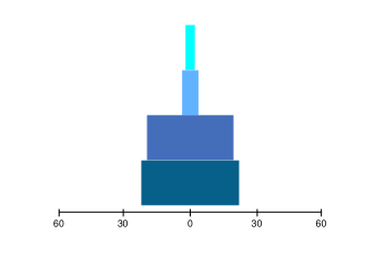
(c)     (d)

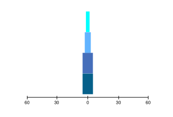
Figure 5: Ecosystem profiles (mean number of species in each trophic level) for increasing $\eta/\xi$ ratios. This plot corresponds to a resource saturation $R=1340$, for which communities have up to 4 trophic levels. Lower levels are shown with darker color. (a) The ecosystem maintain its pyramidal structure ($\eta/\xi=0.05$). (b) The first trophic level starts to collapse ($\eta/\xi=0.3$). (c) The second level starts to loose species ($\eta/\xi=0.43$). (d) For large values of the ratio, the system is close to extinction ($\eta/\xi=0.6$).

A second signal of the transition in this model is a gradual loss of species in trophic levels from bottom to top. This effect can be qualitatively observed in the ecosystem profile (see Figure 5), where the average number of species at each trophic level is shown. When the quotient of rates increases from $\eta/\xi=0.3$ [panel (b)] to $\eta/\xi=0.43$ [panel (c)], the number of species in the first level decreases considerably, but the rest of levels remain almost unaltered. After that [panel (d)], a simultaneous loss of species in the first and second levels takes place.

Figure 6 shows the number of species at each level averaged over $\mathcal{G}$ versus $\eta/\xi$. We observe that the decrease of $s_{1}$ approximately coincides with the first peak of $\sigma_{S}^{2}$ at $\eta_{1}$, and the decrease of $s_{2}$ corresponds to the second peak at $\eta_{2}$. After that, species at lower levels are unable to sustain upper levels and a trophic cascade occurs. The third and fourth levels start to be emptied near $\eta_{3}$. There is a clear correspondence between the values at which trophic levels start to collapse and the location of the maxima of $\sigma_{S}^{2}$ and $\sigma_{T}^{2}/T^{2}$. In any case, the loss of species from bottom to top as the extinction rate increases is a clear signal of the catastrophic regime shift. Besides, trophic cascades have been recognized empirically as signals of over-fishing in marine communities [15].

Figure 6: Average number of species at each trophic level, $s_{\ell}=\sum_{i\in\mathcal{G}}\pi_{i}s_{\ell}^{(i)}$, for $\ell=1,2,3,4$ and $R=1340$, normalized by the average number of species for $\eta=0$, $s_{\ell}(0)$. We have marked the points $\eta_{1}$ and $\eta_{2}$ corresponding to the maxima of $\sigma_{S}^{2}$, which roughly coincide with the points at which the first and second levels start to collapse. The species loss in the third and fourth levels starts when the probability $P_{\varnothing}$ becomes appreciable (by $\eta_{3}$, the maximum of $\sigma_{T}^{2}/T^{2}$).

In the remaining of the section we will consider the variation of $\eta$ as a non-equilibrium process. Now we shall assume that, although the variation of $\eta$ is still not faster than $\xi^{-1}$, the two scales are comparable in the sense that the process is not able to remain in the steady state anymore. An estimate of the time scale for the convergence to the steady state is provided by

$$\xi t_{\rm c}=-\frac{1}{\log|\lambda_{2}|},$$ (5)

where $\lambda_{2}$ is the second largest eigenvalue (in modulus) of the stochastic matrix $P$ (see Figure 7). The distance from the probability distribution after $n$ iterations of the Markov chain to the steady state is proportional to $|\lambda_{2}/\lambda_{1}|^{n}$, hence the definition of $t_{\rm c}$ (note that the maximum eigenvalue $\lambda_{1}=1$ since $P$ is a stochastic matrix). For $R=1340$, the number of iterations needed to reach equilibrium near the shift are around $10^{3}$.

The faster variation of $\eta$ is implemented by producing a small change $\Delta\eta$ every $\Delta n<\xi t_{\rm c}$ iterations of the Markov chain. We start by increasing $\eta$ in these increments until reaching an arbitrary value beyond the regime shift. Then we repeat the process by decreasing $\eta$ in the same increments. This way we can track any observable along the cycle, by computing its averages after $k=0,1,\dots$ increments $\Delta\eta$ using the probability distribution

$$\pi(k\Delta\eta/\xi)=\pi(0)P^{\Delta n}(0)P^{\Delta n}(\Delta\eta/\xi)\cdots P^{\Delta n}(k\Delta\eta/\xi),$$ (6)

given any initial distribution $\pi(0)$ at $\eta=0$ (reverse order in matrix products applies for decreasing $\eta$). In Figure 8 the average species richness exhibits a hysteresis cycle. As $\Delta n$ increases this cycle narrows, recovering the quasi-stationary process in the limit $\Delta n\rightarrow\infty$. In this limit the process is reversible and the cycle collapses to the curve of mean number of species shown in Figure 3.

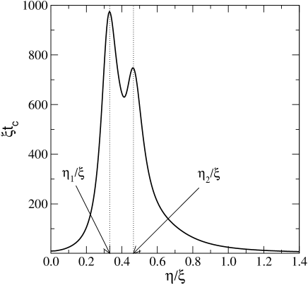
Figure 7: Convergence time $\xi t_{\rm c}=-(\log|\lambda_{2}|)^{-1}$ needed to reach the steady state of the Markov chain, $\lambda_{2}$ being the second largest eigenvalue of matrix $P$. Two peaks appear in $\xi t_{\rm c}$ corresponding to the two maxima of $\sigma_{S}^{2}$.

The existence of hysteresis loops in overexploited systems has been reported in the literature as another signal of catastrophic shifts in ecological communities [7, 12, 14]. We have obtained it for the mean number of species, but a similar behavior will be observed in any other magnitude (like the total biomass density, as in [12]). In spite of the simplicity of our model, hysteresis cycles appear as well as other usual precursors of catastrophic regimes, such as anomalous variance. But, unlike previous models, our model allows a deeper understanding of the transition, as we will discuss below. An important insight this model provides is that hysteresis can arise as a result of a time-scale mixing that keeps the system out of equilibrium rather than to non-linearities of the underlying population model.

4 Phase transition in finite size

As we have mentioned, our model provides a full description of the phase space of the system by means of a transition probability matrix. We are going to take advantage of this fact to show rigorously that the phenomenology that we have described in Section 3 corresponds to a phase transition —in the sense of Statistical Mechanics— in finite size.

In Statistical Mechanics, phase transitions are associated to non-analyticities of the free energy of a physical system. Whenever the system is described by a transfer matrix, the free energy is obtained from its largest eigenvalue. A true phase transition would then be associated to the crossing of the leading eigenvalue with the second largest (in modulus) one, because such a crossing causes a non-analytic behavior of the largest eigenvalue as a function of the control parameter [22]. The counterpart of a transfer matrix in a Markov chain is the transition probability matrix $P$. Thus a crossing of eigenvalues of $P$ would rigorously prove that the system undergoes a phase transition.

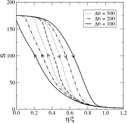
Figure 8: Hysteresis cycles for $\Delta\eta/\xi=0.005$ and three values of $\Delta n$ (see text). Dashed line represents the average number of species in the quasi-stationary process of variation of $\eta$ (for $\Delta n\rightarrow\infty$). The larger $\Delta n$ the further from equilibrium the system and the narrower the cycle.

Strictly speaking, the described shift can not be a true phase transition because of the finiteness of our system. According to the Perron-Frobenius theorem, an irreducible matrix with non-negative entries has a unique largest real eigenvalue and its corresponding eigenvector has strictly positive components [23]. Reducible matrices are related to processes with transient states. Since the Markov chain is ergodic for $\eta>0$, its stochastic matrix $P$ it is irreducible. Then the theorem implies that its maximum eigenvalue $\lambda_{1}=1$ is simple for any value of $\eta/\xi$ (its corresponding positive left eigenvector is precisely the asymptotic probability distribution). This excludes any eigenvalue crossing, therefore any phase transition. True phase transitions can only occur in infinite states Markov chains. When the limiting chain of a sequence of finite Markov chains develops an eigenvalue crossing —hence a phase transition— the second largest eigenvalue of the elements of this sequence approaches the largest one near the location of the true phase transition, the more so the larger the size (number of states) of the Markov chain. This is the fingerprint of the phase transition in finite systems. It is also associated to a qualitative change in the eigenvector associated to the leading eigenvalue.

Figure 9: First (dashed line) and second (full line) eigenvalues of $P$ for a resource saturation $R=1340$. Inset shows a zoom of the region for which $\lambda_{1}=1$ and $\lambda_{2}$ are closest, and two maxima appear at $\eta_{1}/\xi=0.330520\dots$ and $\eta_{2}/\xi=0.462633\dots$. These points coincide with the maxima observed in $\sigma_{S}^{2}$ and $t_{\rm c}$ (see Figure 3 and Figure 7).

We have computed the 10 largest eigenvalues of $P$ (in modulus) using Arnoldi iteration [24] (useful for computing a few eigenvalues of large sparse matrices). In all cases the numerical method provides a real second eigenvalue. Figure 9 shows the dependence of $\lambda_{2}$ as a function of $\eta/\xi$ for $R=1340$. Not surprisingly, we identify the transition points as those of closest approach to the first eigenvalue (i.e., the two maxima observed in $\lambda_{2}$). Those maxima are reached at $\eta_{1}/\xi=0.330520\dots$ and $\eta_{2}/\xi=0.462633\dots$, which coincide with the values observed for the peaks in $\sigma_{S}^{2}$ and $t_{\rm c}$ (see Section 3). As we have shown before, each transition yields a trophic cascade in the system, whose levels get emptied from bottom to top.

We have varied the system size (controlled by the amount of resource, $R$ [18]) in order to check that the second eigenvalue gets closer to the first one as size increases. The system size is measured by the average number of species in the recurrent set for $\eta=0$, and we do observe that the larger the system size the closer is $\lambda_{2}$ to 1 (see Figure 10). It is difficult to increase the size beyond $S\approx 300$ because the number of nodes in $\mathcal{G}$ grows approximately as $e^{\kappa\sqrt{R}}$ [18]. For $S\approx 300$ the number of viable communities is larger than $10^{6}$, and the eigenvalue computation becomes very demanding.

To conclude this section, we have obtained the phase diagram of this system. In Figure 11 we show in a $\eta/\xi$ vs. $R$ diagram the points at which $\lambda_{2}$ reaches its maxima, yielding the transition lines corresponding to the different trophic cascades of the system. Basically transition lines are horizontal, and the number of undergone trophic cascades appears to be related to the number of trophic levels of the communities. We believe that, at some point in the region in which communities have 5 trophic levels, a third maximum would appear related to a separate trophic cascade at the third level. Bearing this hypothesis out is difficult, though, because it would require eigenvalue calculations with too large matrices.

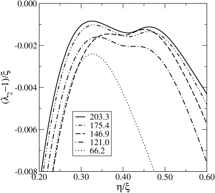
Figure 10: Second eigenvalue of $P$ for several values of $R$ (legend shows the average number of species for each $R$ at $\eta=0$). Dotted curve corresponds to $R=465$, for which the system only allows three trophic levels and only a single maximum is observed. For higher values of $R$ (which allow up to 4 levels), a second maximum appears, related to the trophic cascade in the second level. As the system size increases, $\lambda_{2}$ gets closer to 1.

All this analytical evidence allows us to claim that these model ecosystems undergo a catastrophic transition driven by the relative extinction rate. The dependence of $\lambda_{2}$ with $\eta/\xi$ actually exhibits two maxima and so does the variance in species number. This points towards the existence of a double phase transition, each one associated to a trophic cascade that collapses the lowest and next-to-lowest trophic level in the ecosystem. Increasing the external stress over the system above these values increases the probability of driving the ecosystem to extinction. Consequently there is a threshold in $\eta/\xi$ above which the extinction of the ecosystem is the most likely event. Small variations in that region can cause the collapse of stable ecosystems.

5 Conclusions

In this paper we have used a recently introduced model [16] to propose an alternative explanation to the observed catastrophic regime shifts in overexploited ecosystems [7, 12]. Previous models postulate nonlinearities in the dynamics of a magnitude representative of the whole ecosystem, like for instance the total biomass density, and this non-linear behavior leads to bi-stability. The system undergoes a transition due to a change of regime that leads the system from one stable state to another. This viewpoint is almost the same used in the classical explanations of the liquid-vapor transition in thermodynamics, for which the potential of the system has two alternative stable states.

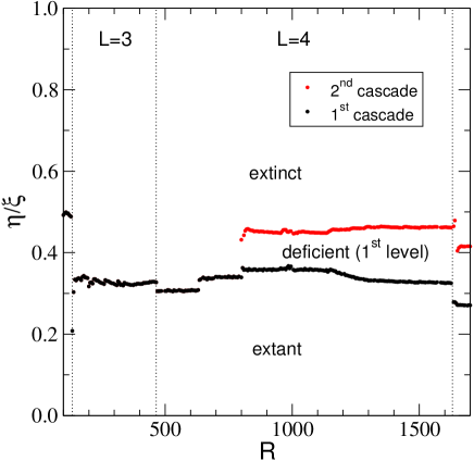
Figure 11: Phase diagram of the system: black circles correspond to the abscissa of the first maximum of $\lambda_{2}$ (trophic cascade at the first level), and red ones to the second maximum (trophic cascade at the second level). Above the second transition, the process stays in communities close to the extinct ecosystem.

Our model, however, is inspired in a microscopic description, more related to the perspective of Statistical Mechanics. Our viable communities are micro-states in a finite phase space and represent different states of the ecosystem. The transition between a species-rich attractor (the recurrent set at $\eta=0$) and an attractor with low number of species (communities close to the empty ecosystem) is explained as the crossing of two eigenvalues of the transition matrix of the Markov chain. This transition is driven by an increasing external force represented by a background species extinction rate, that takes into account the overall mortality for reasons other than predation (overexploitation, habitat destruction, epidemics…).

In spite of its being minimalistic, the model reproduces qualitatively the phenomenology observed in overexploited ecosystems. We have studied for this model the behavior of several early-warnings that announce the catastrophic shift, and we have found the same behavior as that obtained both in previous models [7, 12] and empirically [14]. These features are shared by many systems under the framework of the elementary catastrophe theory [25].

Catastrophes have characteristic fingerprints. Some of the standard flags of catastrophic regimes are modality, anomalous variance and hysteresis [26]. These are precisely the signals we find in our model. Our system is bimodal because it undergoes transitions between an attractor of high species richness to another stable state with low species richness. Fluctuations in the mean number of species exhibit peaks at the transition points, and take very large values compared to their values far away from the transition. We thus have anomalous behavior of variances. And the average number of species exhibits hysteresis cycles when the system is kept out of equilibrium, as we have shown in Section 3. This explanation of hysteresis is alternative to the existence of non-linearities in the population model, and points towards the speed of variation of the external stress. The difference with the usual explanation is that in this case the ecosystem can recover its initial state after releasing the external stress, provided that we wait long enough and that there is availability of invaders.

The main advantage of our model is the microscopic description that it provides. The full characterization of the phase space of the system has allowed us to show rigorously that the system undergoes a true phase transition by computing the second eigenvalue of the transition matrix, which gets closest to the first eigenvalue in the vicinity of the transition. This provides a theoretical support to the critical behavior exhibited by magnitudes like the fluctuation of species richness.

We have found evidence for a double phase transition in the system, associated to the gradual loss of species from bottom to top. This effect is new to former models and could be used as early warning for the catastrophic shift by monitoring the species abundance at low trophic levels in overexploited ecosystems. Trophic cascades have been revealed as possible mechanisms of catastrophic shifts in natural communities, though [15]. Thus, with the caveat that this is just a very simplified picture of real communities, our analysis of this model predicts that overexploited systems will begin to collapse first at lower levels.

Assuming a different extinction rate at each trophic level would be more realistic. For example, in overexploited marine ecosystems, the impact of fishing pressure is stronger in higher trophic levels. A simple model like ours could shed light in determining whether a strong extinction pressure in higher levels is more harmful than in lower levels. Refined versions of the model could allow investigating this kind of effects.

Most theoretical explanations of the catastrophic phenomena observed in ecological systems subject to high exploitation pressure rely on nonlinearities in the macroscopic dynamics of the system. The take-home message of this paper is that a microscopic model like ours, based in ecologically reasonable assumptions and in a simple, linear population dynamic models, can exhibit the same phenomenology as non-linear, macroscopic models. This way, our approach can serve as an alternative explanation of the catastrophic regime shifts observed in ecological communities.

Appendix

This appendix is devoted to calculate the fluctuation of the average time of first return to the empty ecosystem. Throughout this section $f_{ij}^{(n)}$ will stand for the probability that in a process starting form the state $i$ the first entry to $j$ occurs after $n$ steps. The distribution $\{f^{(n)}_{ij}\}$ is known as the first-passage distribution for the state $j$ (in particular, $\{f^{(n)}_{jj}\}$ represents the distribution of the recurrence times for $j$). This distribution is related to the probabilities $p_{ij}^{(n)}$ of a transition from $i$ to $j$ in exactly $n$ steps [21] according to

$$p_{ij}^{(n)}=\sum_{\nu=1}^{n}f_{ij}^{(\nu)}p_{jj}^{(n-\nu)}.$$ (7)

Let us study the case $i=j=\varnothing$. We are interested in calculating the variance of the recurrence time for the empty community, whose mean value is given by $T=\sum_{n=1}^{\infty}nf_{\varnothing\varnothing}^{(n)}$. To this purpose we introduce the generating functions $V(z)=\sum_{n=0}^{\infty}p_{\varnothing\varnothing}^{(n)}z^{n}$ ($p_{\varnothing\varnothing}^{(0)}=1$) and $F(z)=\sum_{n=0}^{\infty}f_{\varnothing\varnothing}^{(n)}z^{n}$ ($f_{\varnothing\varnothing}^{(0)}=0$). Then (7) is equivalent [21] to

$$F(z)=1-\frac{1}{V(z)}$$ (8)

and $T=F^{\prime}(1)$. It can be easily shown that the radius of convergence of $V(z)$ is equal to 1, and that $V(1)$ diverges by definition. By imposing that $F^{\prime}(1)$ is finite we find that, near $z=1$, $V(z)\approx a(1-z)^{-1}$ and $a=\lim_{n\rightarrow\infty}p_{\varnothing\varnothing}^{(n)}=P_{\varnothing}$. Hence the mean recurrence time for $\varnothing$ is $T=F^{\prime}(1)=a^{-1}=P_{\varnothing}^{-1}$.

The variance of the recurrence time is obtained as

$$\sigma_{T}^{2}=\sum_{n=0}^{\infty}n^{2}f_{\varnothing\varnothing}^{(n)}-T^{2}=F^{\prime\prime}(1)-F^{\prime}(1)[1-F^{\prime}(1)].$$ (9)

In order to calculate $F^{\prime\prime}(1)$, we need to obtain the next-to-leading (constant) term in the series expansion of $V(z)$ in powers of $1-z$, $V(z)=P_{\varnothing}(1-z)^{-1}+b+\mathcal{O}(1-z)$. Using (8) we get $F^{\prime\prime}(1)=2b/P_{\varnothing}^{2}$ and

$$\frac{\sigma_{T}^{2}}{T^{2}}=2b+P_{\varnothing}-1.$$ (10)

To conclude with this calculation, we need to obtain a way to compute numerically the constant $b$. This is an easy task, because

$$b+\mathcal{O}(1-z)=V(z)-\frac{P_{\varnothing}}{1-z}=\sum_{n=0}^{\infty}\left(p_{\varnothing\varnothing}^{(n)}-P_{\varnothing}\right)z^{n}.$$ (11)

Hence, in the limit $z\rightarrow 1$,

$$b=\sum_{n=0}^{\infty}\left(p_{\varnothing\varnothing}^{(n)}-P_{\varnothing}\right).$$ (12)

Therefore we simply need to iterate the matrix $P$ and truncate the series up to certain error tolerance to compute $b$.

References

References

- [1] David Tilman, Joseph Fargione, Brian Wolff, Carla D’Antonio, Andrew Dobson, Robert Howarth, David Schindler, William H. Schlesinger, Daniel Simberloff, and Deborah Swackhamer. Forecasting agriculturally driven global environmental change. Science, 292:281–284, 2001.
- [2] Marten Scheffer, Sándor Szabó, Alessandra Gragnani, Egbert H. van Nes, Sergio Rinaldi, Nils Kautsky, Jon Norberg, Rudi M. M. Roijackers, and Rob J. M. Franken. Floating plant dominance as a stable state. Proc. Nat. Acad. Sci., 100:4040–4045, 2003.
- [3] T. J. Done. Phase shifts in coral reef communities and their ecological signifcance. Hydrobiologia, 247:121–132, 1991.
- [4] Magnus Nystrom, Carl Folke, and Fredrik Moberg. Coral reef disturbance and resilience in a human-dominated environment. Trends Ecol. Evol., 15:413–417, 2000.
- [5] Brian H. Walker. Rangeland ecology: Understanding and managing change. Ambio, 22:80–87, 1993.
- [6] Donald Ludwig, Brian Walker, and Crawford S. Holling. Sustainability, stability, and resilience. Conserv. Ecol., 1(1):7, 1997.
- [7] Marten Scheffer amd Steve Carpenter, Jonathan A. Foley, Carl Folke, and Brian Walker. Catastrophic shifts in ecosystems. Nature, 413:591–596, 2001.
- [8] Robert M. May. Thresholds and breakpoints in ecosystems with a multiplicity of stable states. Nature, 269:471–477, 1977.
- [9] Chih hao Hsieh amd Christian S. Reiss, John R. Hunter, John R. Beddington, Robert M. May, and George Sugihara. Fishing elevates variability in the abundance of exploited species. Nature, 443:859–862, 2006.
- [10] Christian N. K. Anderson, Chih hao Hsieh, Stuart A. Sandin, Roger Hewitt, Anne Hollowed, John Beddington, Robert M. May, and George Sugihara. Why fishing magnifies fluctuations in fish abundance. Nature, 452:835–839, 2008.
- [11] Donald Ludwig, Dixon D. Jones, and Crawford S. Holling. Qualitative analysis of insect outbreak systems: the spruce budworm and forest. J. Anim. Ecol., 47:315–332, 1978.
- [12] Ariel Fernández and Hugo Fort. Catastrophic phase transitions and early warnings in a spatial ecological model. J. Stat. Mech., 9:09014–21, 2009.
- [13] Vasilis Dakos, Egbert H. van Nes, Raúl Donangelo, Hugo Fort, and Marten Scheffer. Spatial correlation as leading indicator of catastrophic shifts. Theor. Ecol., 3:163–174, 2010.
- [14] Marten Scheffer, Jordi Bascompte, William A. Brock, Victor Brovkin, Stephen R. Carpenter, Vasilis Dakos, Hermann Held, Egbert H. van Nes, Max Rietkerk, and George Sugihara. Early-warning signals for critical transitions. Nature, 461:53–59, 2009.
- [15] Georgi M. Daskalov, Alexander N. Grishin, Sergei Rodionov, and Vesselina Mihneva. Trophic cascades triggered by overfishing reveal possible mechanisms of ecosystem regime shifts. Proc. Natl. Acad. Sci., 104:10518–10523, 2007.
- [16] José A. Capitán, José A. Cuesta, and Jordi Bascompte. Statistical mechanics of ecosystem assembly. Physical Review Letters, 103:168101–4, 2009.
- [17] José A. Capitán and José A. Cuesta. Species assembly in model ecosystems, i: Analysis of the population model and the invasion dynamics. arXiv:1006.5560v1, 2010.
- [18] José A. Capitán, José A. Cuesta, and Jordi Bascompte. Species assembly in model ecosystems, ii: Results of the assembly process. arXiv:1006.5562v1, 2010.
- [19] Richard Law and R. Daniel Morton. Permanence and the assembly of ecological communities. Ecology, 77:762–775, 1996.
- [20] R. Daniel Morton and Richard Law. Regional species pools and the assembly of local ecological communities. J. Theor. Biol., 187:321–331, 1997.
- [21] William Feller. An introduction to probability theory and its applications, vol. 1. Wiley, New York, 1968.
- [22] José A. Cuesta and Angel Sánchez. General non-existence theorem for phase transitions in one-dimensional systems with short range. J. Stat. Phys., 115:869–893, 2004.
- [23] Carl D. Meyer. Matrix Analysis and Applied Linear Algebra. SIAM, Philadelphia, 2000.
- [24] Lloyd N. Trefethen and David Bau. Numerical Linear Algebra. SIAM, Philadelphia, 1997.
- [25] René Thom. Structural Stability and Morphogenesis. Benjamin, Reading, Massachusetts, 1975.
- [26] Robert Gilmore. Catastrophe Theory for Scientists and Engineers. Dover, New York, 1981.