Adaptive Oscillator Networks with Conserved Overall Coupling: Sequential Firing and Near-Synchronized States

Abstract

Motivated by recent observations in neuronal systems we investigate all-to-all networks of non-identical oscillators with adaptive coupling. The adaptation models spike-timing-dependent plasticity in which the sum of the weights of all incoming links is conserved. We find multiple phase-locked states that fall into two classes: near-synchronized states and splay states. Among the near-synchronized states are states that oscillate with a frequency that depends only very weakly on the coupling strength and is essentially given by the frequency of one of the oscillators, which is, however, neither the fastest nor the slowest oscillator. In sufficiently large networks the adaptive coupling is found to develop effective network topologies dominated by one or two loops. This results in a multitude of stable splay states, which differ in their firing sequences. With increasing coupling strength their frequency increases linearly and the oscillators become less synchronized. The essential features of the two classes of states are captured analytically in perturbation analyses of the extended Kuramoto model used in the simulations.

I Introduction

Understanding the collective dynamics of coupled oscillators is an important issue in nonlinear dynamics. In particular the coherence and synchronization of oscillators is relevant in many areas of science and technology. Well-studied physical examples are arrays of Josephson junctions (e.g. StMi93 ) and lasers (e.g. SiFa93 ), where synchronization is often desired since it can enhance the output power of devices. The understanding of synchronization of oscillators has also informed the development of control for groups of self-propelled agents SePa05 . Classical biological examples for oscillator arrays are networks of neurons. The coherence and synchronization of neural spiking within such ensembles of neurons underlies various types of rhythmic activity, which have been associated with a variety of brain functions BuDr04a . Thus, the communication between different brain areas can be enhanced during certain phases of their rhythms, which may allow to limit effective communication to areas whose rhythms are (transiently) coherent Fr05 . Rhythms like theta- or gamma-oscillations can provide a ‘clock’ that allows information to be encoded in terms of the timing of neuronal spikes relative to the phase of the ensemble oscillation ScAn06 . For various brain functions it has been reported that the relevant information is carried by correlations between neuronal spiking rather than by their mean firing rate VaHa95 ; DeMe96 . In other situations it is not desired that neurons fire in near synchrony but rather in a specific sequence. This is, for instance, the case for networks serving as central pattern generators that control the movement of limbs in legged locomotion GoSt99 ; CaBu97 and for networks controlling the production of bird songs FiSe10 .

A unified description of the dynamics of coupled oscillators is possible if the coupling is sufficiently weak. The interaction between oscillators affects then predominantly their phase and the system can be described as a network of phase oscillators Ne79a ; HaMa95 ; Er96 . Their interaction is determined by the phase resetting curve Er96 ; HaMa95 , which results from the impact of the synaptic coupling on the dynamics of the individual oscillators. In the limit of weak coupling the interaction simplifies significantly and depends only on the difference between the oscillator phases. A minimal model of this type is the classic Kuramoto model Ku84b ; St00 , in which the interaction is taken to be purely sinusoidal. It has provided an excellent framework for understanding the onset of synchronization in globally coupled networks of oscillators with different natural frequencies.

In particular in biological systems the properties of the interacting elements themselves as well as their interactions need not be constant in time; often they evolve on slower time scales in response to the dynamics of the system. In networks of neurons synaptic plasticity, i.e. the modification of their coupling strengths, is a widely observed mechanism that endows the system with the ability to learn, to memorize, and to adapt to variable environments. In one well-established type of synaptic plasticity the modification of the coupling strength depends on the timing of the pre-synaptic input and the post-synaptic activity. Typically, the coupling strength is potentiated if the pre-synaptic neuron provides synaptic input before the post-synaptic neuron spikes, while in the converse case the synaptic strength is depressed CaDa08 . For neural oscillators this tends to enhance the impact of faster oscillators on the slower ones and weaken the converse influence. The effect of such a spike-timing dependent plasticity (STDP) on the synchronization of (neural) oscillators has been studied by a number of authors employing extensions of the Kuramoto model. It was found that the plasticity can enhance the synchronization of oscillators KaEr02 . Moreover, for coupling strengths that are sufficient to render all oscillators phase-locked to each other this type of plasticity was found to lead to only a single completely phase-locked state. Its effective network structure has no loops and its frequency is given by that of the fastest oscillator MaLy07 .

Synaptic plasticity need not always be homosynaptic, i.e. the modification of the strength of a given synapse need not depend only on the activity of the neurons connected by that synapse. Instead, various situations have been identified in which the strength $K_{ij}$ of the synapse from neuron $j$ onto neuron $i$ is modified also in response to the activity of other neurons $l\neq j$ that synapse onto neuron $i$ (heterosynaptic plasticity). In particular, it has been found that the potentiation of synapse $K_{il}$ can lead to the depression or depotentiation of synapse $K_{ij}$ FoNa04 . In addition, in some preparations also the converse was observed; there depression of synapse $K_{il}$ led to the potentiation of synapse $K_{ij}$ RoPa03 . Moreover, for that system evidence was presented that suggested that the sum of the weights of all incoming synapses remained essentially constant despite the changes in the individual synapses RoPa03 . Recently, similar observations were made on an anatomical level, where the combined size of all synapses on a dendritic segment was found to be constant, while individual synapses grew or shrank in response to potentiating stimuli BoHa10 .

Motivated by the observation of heterosynaptic plasticity that approximately preserves the total weight of all incoming synapses RoPa03 , we investigate here a minimal model of neural oscillators with spike-timing dependent plasticity that conserves the total incoming weight. Heterosynaptic plasticity introduces competition between the synapses and the weight conservation implies that even the fastest oscillator, which ends up without any inputs in the case of the usual STDP rule, receives inputs and the network of effectively coupled oscillators develops loops. We find that this leads to qualitative changes in the dynamics of the network. In particular, we find not only a single state in which all oscillators are phase-locked but a host of such states. They fall into two classes: near-synchronous states and splay states. Depending on the shape of the plasticity function we find a number of different near-synchronous states, characterized by different dependencies of the frequency on the overall coupling strength. Among them are states whose frequency is essentially given by that of one of the oscillators in the network. In contrast to the case of purely homosynaptic plasticity MaLy07 this is, however, not the fastest oscillator but an intermediate one. In the phase-locked splay states the phases are distributed quite homogeneously over the whole range $[0,2\pi]$. While typically the order parameter that characterizes the synchronization of the oscillators increases with coupling strength, in these splay states it decreases and the oscillators become less synchronized with increasing coupling strength. In a neural context splay states correspond to states of the network in which the neurons fire in sequence spread over the whole period of the network oscillation. We find that the firing sequence of the splay states depends sensitively on the initial conditions, leading to a large number of stably coexisting splay states differing in their firing sequence.

The splay states exhibit parallels to the states with sequential firing obtained in FiSe10 . There it was found that networks of excitable neurons with a related type of heterosynaptic plasticity can produce firing sequences that match important aspects of the neural activity observed during the production of bird songs.

The paper is organized as follows. In Section 2 we discuss the oscillator model and its connection to general oscillators and we introduce a plasticity rule that reflects spike-timing-dependent plasticity and conservation of incoming weights. In Section 3 we consider networks with few oscillators and complement the numerical simulations with a perturbation analysis that reveals the origin of the transitions between different phase-locked regimes. In Section 4 we investigate larger networks. They allow a multitude of different phase-locked states, including many stably coexisting splay states. We capture the characteristics of the simplest splay states with another analytical perturbation calculation. Conclusions are presented in Section 5.

II The Model

We consider a network of $N$ oscillators with plastic interactions in which the sum of all incoming weights is conserved. For the form of the interaction we assume that for sufficiently small frequency differences pairs of oscillators phase-lock close to synchrony. For weak coupling such a network can be described in terms of the phases $\theta_{i}$ of the oscillators,

$$\dot{\theta}_{i}=\omega_{i}-\frac{1}{N}\sum_{i\neq j=1}^{N}K_{ij}H_{ij}\left(\theta_{i}-\theta_{j}\right),\qquad i=1,\ldots,N,$$ (1)

with the $2\pi$-periodic interaction function $H(\theta_{i}-\theta_{j})$ depending only on the phase differences HaMa95 ; Er96 . In the following we assume $\omega_{i}<\omega_{j}$ for $i<j$. While we allow the oscillators to have different natural frequencies we assume for simplicity that they are identical in all of their other properties. In particular, we assume that they all have the same interaction function, $H_{ij}(\Delta\theta)=H(\Delta\theta)$ and the same value of the sum of all incoming weights,

$$\hat{K}=\sum_{i\neq j=1}^{N}K_{ij}.$$ (2)

The focus of this paper are solutions in which the oscillators are phase-locked to each other with small phase differences. The existence and linear stability of those states is affected only by the leading-order expansion of $H(\theta)$ around $\theta=0$, $H(\Delta\theta)=h^{(0)}+h^{(1)}\Delta\theta+h.o.t.$ Since the sum of all incoming weights is conserved, the contribution $h^{(0)}$ can be absorbed in the frequency of each oscillator, $\omega_{i}\rightarrow\omega_{i}-h^{(0)}\hat{K}$. Since pairs of oscillators are assumed to phase-lock close to synchrony for small frequency differences the coefficient $h^{(1)}$ has to be positive and can be absorbed into $K_{ij}$. As a minimal model for the phase evolution we therefore use the classic Kuramoto-model Ku84b ; St00 , which has the same leading-order behavior in $\theta_{i}-\theta_{j}$,

$$\dot{\theta}_{i}=\omega_{i}-\frac{1}{N}\sum_{i\neq j=1}^{N}K_{ij}\sin\left(\theta_{i}-\theta_{j}\right),\qquad i=1,\ldots,N.$$ (3)

Even for systems with general interaction functions $H(\Delta\theta)$ the Kuramoto model will capture the existence and linear stability of solutions in which all phase differences are small. Their basins of attraction will not be properly represented, however, nor will be solutions that are characterized by $\mathcal{O}(1)$ phase differences.

For the modifiable interactions we consider coupling strengths $K_{ij}$ that evolve depending on the phases of the interacting oscillators,

$$\tau\dot{K}_{ij}=f\left(K_{ij},\theta_{i},\theta_{j}\right)-K_{ij}\frac{\sum_{i\neq l=1}^{N}f\left(K_{il},\theta_{i},\theta_{l}\right)}{\sum_{i\neq l=1}^{N}K_{il}}.$$ (4)

The weight evolution of a single synaptic connection would be given by $f\left(K_{ij},\theta_{i},\theta_{j}\right)$. The second term in (4) expresses the conservation of the total weight of all incoming connections of an oscillator. Instead of this instantaneous conservation one could also consider achieving homeostasis of the total weight on a longer time scale ZhLa06 . The existence of the phase-locked states that we are interested in here would not be affected by such a slower evolution, since they correspond to fixed-points of (4). At most, such a delayed homeostasis could influence their stability.

We assume that the weights evolve on a slow time scale, $\tau\gg 1$, and change only little during one period of oscillation of the interacting oscillators. Due to averaging the weight changes depend then to leading order only on the phase difference $\theta_{i}-\theta_{j}$ GuHo83 . For the plasticity function $f(K_{ij},\theta_{i}-\theta_{j})$ we use a functional form that is motivated by the widely observed spike-timing dependent plasticity (STDP) of neuronal oscillators BiPo98 . There a synaptic connection is potentiated when the pre-synaptic neuron spikes before the post-synaptic one and depressed otherwise. Within the present phase framework this corresponds to a potentiation when the phase of the pre-synaptic oscillator is larger than that of the post-synaptic oscillator. Specifically we use

$$f\left(K_{ij},\theta_{i},\theta_{j}\right)=\begin{cases}\left(\alpha-K_{ij}\right)e^{\frac{\theta_{i}-\theta_{j}}{\tau_{p}}}&\quad\mbox{for }\theta_{i}-\theta_{j}\in(-\pi,-\psi)\\ \beta_{0}+\beta_{1}\left(\theta_{i}-\theta_{j}\right)&\quad\mbox{for }\theta_{i}-\theta_{j}\in[-\psi,\psi]\\ -K_{ij}e^{-\frac{\theta_{i}-\theta_{j}}{\tau_{d}}}&\quad\mbox{for }\theta_{i}-\theta_{j}\in(\psi,\pi]\end{cases},$$ (5)

where $\theta_{i}-\theta_{j}$ is taken modulo $2\pi$ within the range $(-\pi,\pi]$. We include a central phase window $[-\psi,\psi]$ within which potentiation and depression are continuously interpolated AbHu02 . Typically, we will assume this window to be narrow, $\psi\ll\tau_{d,p}$ or even $\psi=0$. The coefficients $\beta_{0,1}$ are given by

$$\beta_{0} = \frac{1}{2}e^{-\frac{\psi}{\tau_{p}}}\left(\alpha-K_{ij}\right)-\frac{1}{2}K_{ij}e^{-\frac{\psi}{\tau_{d}}},$$

$$\beta_{1} = \frac{1}{2\psi}\left\{\left(K_{ij}-\alpha\right)e^{-\frac{\psi}{\tau_{p}}}-K_{ij}e^{-\frac{\psi}{\tau_{d}}}\right\}.$$

Figure 1: Plasticity function $f(K_{ij},\theta_{i}-\theta_{j})$ for $\alpha=10$, $\psi=0.02$ , $\tau_{d,p}=0.1$, $K_{ij}=5.89$. The coupling strength is increased if the phase $\theta_{j}$ of the presynaptic oscillator is larger than the phase $\theta_{i}$ of the postsynaptic oscillator, $\Delta\theta=\theta_{i}-\theta_{j}<0$.

Our main control parameter is the sum $\hat{K}$ of all incoming weights. The parameter $\alpha$ sets the maximal strength of an individual synapse in the absence of the homeostatic term in (5). We focus here on phenomena that are dominated by the limitation of the overall coupling $\hat{K}$ and choose $\alpha$ well above $\hat{K}$. Note, however, that due to the homeostatic, second term in (4) the coupling strengths $K_{ij}$ are not strictly limited to $K_{ij}\leq\alpha$. Correspondingly, we did not find qualitatively different behavior when $\alpha$ was chosen somewhat below $\hat{K}$.

III Few Oscillators

For oscillator networks in which the plastic coupling is not conserved it was found that for arbitrary network sizes there is only a single phase-locked state and the transition from the incoherent states to that phase-locked state is hysteretic only if the plasticity windows $\tau_{p,d}$ for potentiation and depression are not equal MaLy07 . We find that with the conservation of the overall input strength hysteresis arises even with equal plasticity windows. Moreover, the transition scenario and the extent of hysteresis depends strongly on the natural frequencies of the oscillators. The case of three oscillators is illustrated in Fig.2. Depending on $\omega_{2}$ with $\omega_{1,3}$ fixed, all three oscillators can phase lock in what seems a single hysteretic transition ($1.2\leq\omega_{2}\leq 1.5$) or in two subsequent transitions with an intermediate, partially phase-locked state ($1.6\leq\omega_{2}\leq 1.9$).

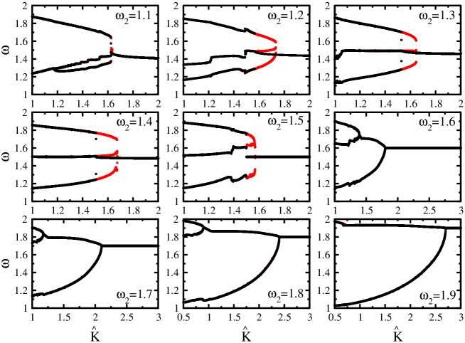
Figure 2: Transition sequences to the phase-locked states for $N=3$ oscillators for different values of the intermediate frequency $\omega_{2}$. Parameters: $\tau=20$, $\tau_{d}=\tau_{p}=0.3,$ $\omega_{1}=1$, $\omega_{3}=2$, $\alpha=100$, $\psi=0$. For $\omega_{2}>1.5$ the frequency of the phase-locked state is very close to $\omega_{2}$ (cf. Fig.3). Red symbols denote increasing $\hat{K}$, black symbols decreasing $\hat{K}$.

A particularly striking aspect of the simulations shown in Fig.2 is that the frequency $\omega$ of the completely phase-locked state exhibits two different regimes: for $\omega_{2}$ closer to the lower frequency $\omega_{1}$ the frequency $\omega$ depends only little on $\omega_{2}$, while for $\omega_{2}$ closer to the larger frequency $\omega_{3}$ the three oscillators oscillate at a frequency that is very close to the natural frequency $\omega_{2}$ of the second fastest oscillator. This is shown more explicitly in Fig.3. We find this surprising selection of the frequency of the second-fastest oscillator also in simulations with more oscillators (see below).

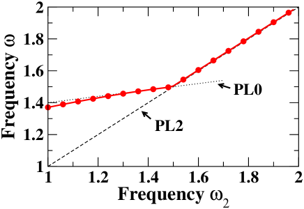
Figure 3: Dependence of the frequency of the phase-locked state on the frequency of the second oscillator, $\omega_{2}$, for $\hat{K}=3$, $\tau=20$, $\tau_{d}=\tau_{p}=0.3,$ $\omega_{1}=1$, $\omega_{3}=2$, $\alpha=100$, $\psi=0$.005 (cf. Fig.2). The dashed and the dotted line give the analytical results (14) and (19) for the frequency of PL0 and PL2, respectively.

To get an analytic understanding of the regimes found in Fig.2 and in particular to identify the origin for the phase-locking at a frequency close to that of the second-fastest oscillator we consider the situation in which the phase differences $\Delta\theta_{ij}$ are sufficiently small to allow a linearization of the nonlinearities in (1) and (5). We therefore assume that the differences between the three frequencies are small,

$$\omega_{2}=\omega_{1}+\epsilon\Omega_{2},\qquad\omega_{3}=\omega_{1}+\epsilon\Omega_{3},\qquad\epsilon\ll 1,$$ (6)

so that a coupling of $\mathcal{O}(1)$ can lock the phase differences at small values. The phase differences can therefore be expanded as

$$\Delta\theta_{12}=\epsilon\,\delta\theta_{12}^{(1)}+\epsilon^{2}\,\delta\theta_{12}^{(2)}+\mathcal{O}(\epsilon^{3}),\qquad\Delta\theta_{23}=\epsilon\,\delta\theta_{23}^{(1)}+\epsilon^{2}\,\delta\theta_{23}^{(2)}+\mathcal{O}(\epsilon^{3}).$$ (7)

In addition, to avoid that all phase differences fall in the central range $[-\psi,\psi]$ of the plasticity function we assume that range to be narrow,

$$\psi=\epsilon\Psi.$$ (8)

We also expand the coupling coefficients,

$$K_{ij}=K_{ij}^{(0)}+\epsilon K_{ij}^{(1)}+\mathcal{O}(\epsilon^{2})$$ (9)

The piecewise definition of the plasticity function $f\left(K_{ij},\theta_{i},\theta_{j}\right)$ in (5) requires that one distinguishes different cases depending on $\Delta\theta_{ij}\equiv\theta_{i}-\theta_{j}$. For $\Omega_{3}-\Omega_{2}=(\omega_{3}-\omega_{2})/\epsilon$ and $\Omega_{2}-\Omega_{1}=(\omega_{2}-\omega_{1})/\epsilon$ not too small both phase differences $\Delta\theta_{12}$ and $\Delta\theta_{23}$ fall outside the inner range $[-\psi,\psi]$ of the plasticity function. Inserting the expansions (7,9) into (3,4) leads then in a straightforward fashion to evolution equations for the leading-order contributions $K_{ij}^{(0)}$ and $\delta\theta_{ij}^{(1)}$,

$$\dot{\delta\theta_{32}^{(1)}} = \Omega_{3}-\Omega_{2}+\frac{1}{3}\delta\theta_{32}^{(1)}\left\{K_{21}^{(0)}-2\hat{K}\right\}+\frac{1}{3}\delta\theta_{21}^{(1)}\left\{K_{32}^{(0)}+K_{21}^{(0)}-\hat{K}\right\},$$ (10)

$$\dot{\delta\theta_{21}^{(1)}} = \Omega_{2}+\frac{1}{3}\delta\theta_{32}^{(1)}\left\{\hat{K}-K_{21}^{(0)}-K_{13}^{(0)}\right\}-\frac{1}{3}\delta\theta_{21}^{(1)}\left\{K_{21}^{(0)}+\hat{K}\right\}$$ (11)

and

$$\tau\dot{K}_{32}^{(0)} = -\epsilon\frac{K_{32}^{(0)}\left(\hat{K}-K_{32}^{(0)}\right)\delta_{21}^{(1)}}{\tau_{d}\hat{K}},$$

$$\tau\dot{K}_{21}^{(0)} = -\frac{\alpha}{\hat{K}}K_{21}^{(0)},$$

$$\tau\dot{K}_{13}^{(0)} = \alpha\left\{\hat{K}-2K_{13}^{(0)}\right\}.$$

and an additional equation for one of the phases, $\theta_{1}$ say, which for steady states yields the oscillation frequency $\omega\equiv\dot{\theta}_{1}$. Note that the evolution of $K_{32}^{(1)}$ is slower than that of $K_{21}^{(1)}$ and $K_{13}^{(1)}$. These equations have two fixed points, which represent phase-locked solutions. Only one of them is linearly stable. It is given by

$$\mbox{PL0}:\qquad K_{32}^{(0)}=0\qquad K_{13}^{(0)}=\frac{1}{2}\hat{K}\qquad K_{21}^{(0)}=0$$ (12)

$$\delta\theta_{32}^{(1)}=\frac{6}{5}\frac{\Omega_{3}-2\Omega_{2}}{\hat{K}}\geq\Psi\qquad\delta\theta_{21}^{(1)}=\frac{3}{5}\frac{\Omega_{3}+3\Omega_{2}}{\hat{K}}\geq\Psi$$ (13)

with the remaining coupling coefficients determined through the conservation law, e.g. $K_{23}^{(0)}=\hat{K}-K_{21}^{(0)}.$ This solution is only valid as long as $\delta\theta_{32}^{(1)}\geq\Psi$ and $\delta\theta_{21}^{(1)}\geq\Psi$ as indicated by the inequalities in (13). The oscillation frequency of PL0 is given by

$$\omega=\omega_{1}+\epsilon\left(\frac{2}{5}\Omega_{3}+\frac{1}{5}\Omega_{2}\right)+\mathcal{O}(\epsilon^{2}).$$ (14)

This frequency is not necessarily close to $\omega_{2}$; in fact, it varies only weakly with $\omega_{2}$.

When $\Omega_{3}-2\Omega_{2}<5\hat{K}\Psi/6$ the phase difference $\Delta\theta_{32}^{(1)}$ of PL0 falls into the central range $[-\psi,\psi]$. This modifies the evolution equations for $K_{ij}$ (cf. (4) and (32,33,34) in the appendix) and the expansion (7,9) yields 3 possible phase-locked solutions. They are given by

PL1: $$K_{32}^{(0)}=\hat{K}\qquad K_{13}^{(0)}=\frac{1}{2}\hat{K}\qquad K_{21}^{(0)}=0$$

$$\delta\theta_{32}^{(1)}=\frac{3}{2}\frac{\Omega_{3}-\Omega_{2}}{\hat{K}}\leq\Psi\qquad\delta\theta_{21}^{(1)}=\frac{3}{4}\frac{\Omega_{3}+3\Omega_{2}}{\hat{K}}\geq\Psi$$

with frequency

$$\omega=\omega_{1}+\frac{1}{2}\epsilon\left(\Omega_{2}+\Omega_{3}\right)+\mathcal{O}(\epsilon^{2}),$$ (16)

and

PL2a: $$0\leq K_{32}^{(0)}=\hat{K}\frac{12\Omega_{2}-6\Omega_{3}+5\Psi\hat{K}}{6\Omega_{2}+\Psi\hat{K}}\leq\hat{K}\qquad K_{13}^{(0)}=\frac{1}{2}\hat{K}\qquad K_{21}^{(0)}=0$$ (17)

$$\delta\theta_{32}^{(1)}=\Psi\qquad\delta\theta_{21}^{(1)}=\frac{6\Omega_{2}+\Psi\hat{K}}{2\hat{K}}\geq\Psi$$ (18)

with frequency

$$\omega=\omega_{1}+\epsilon\left(\Omega_{2}+\frac{1}{3}\Psi\hat{K}\right)+\mathcal{O}(\epsilon^{2}),$$ (19)

and a solution PL2b that is obtained from PL2a by interchanging oscillators 2 and 3, keeping in mind that interchanging $\Omega_{2}\leftrightarrow\Omega_{3}$ implies $K_{32}^{(0)}\leftrightarrow K_{23}^{(0)}=\hat{K}-K_{21}^{(0)}$. Again, the range of validity of each solution is indicated by the various inequalities.

The ranges of validity of the solutions PL0, PL1, and PL2a,b are mutually exclusive. In particular, depending on the sign of $\Omega_{3}-\Omega_{2}$ at most one of PL2a and PL2b is valid. Moreover, at the validity limit of the solution PL0, $\Omega_{3}-2\Omega_{2}=5\hat{K}\Psi/6$, it becomes equal to PL2a with $K_{32}^{(0)}=0$, which at the same time represents one limit of validity of PL2a. At the other limit of validity of PL2a one has $K_{23}^{(0)}=\hat{K}$. There it coincides with PL1 at one of its limits of validity. Finally, PL1 reaches its other limit of validity when $\delta\theta_{21}=\Psi$. To continue the solutions into this regime a further expansion would be necessary, in which also $\delta\theta_{21}^{(1)}$ is assumed to be in $[-\Psi,\Psi]$. Thus, we find a single branch of near-synchronous phase-locked solutions, which exhibit, however, quite different behaviors in the different regimes.

Note, that in none of the regimes the oscillators are truly synchronous, i.e. their phase differences do not vanish. This is to be contrasted with previous results on oscillator network models with homo-synaptic plasticity where it had been found that the plasticity can lead to perfect synchronization of the oscillators, although the oscillators have different natural frequencies KaEr02 . In that model the plasticity can effectively induce different values of $H(0)$ for the different oscillators, which can compensate for the differences in natural frequencies even for $\Delta\theta_{ij}=0$. With conserved total incoming weights, however, the plastic modification of $H(0)$ is the same for all oscillators and perfect synchrony cannot be achieved.

The quantitative comparison of the perturbation analysis and the numerical simulations presented in Fig.3 shows that PL0 and PL2a capture the phase-locked states obtained in Fig.2. Thus, the perturbation analysis reveals that phase-locking of the three oscillators at a frequency very close to that of the second fastest oscillator is obtained if the transition region between potentiation and depression is narrow, $\psi\ll 1$.

To investigate the additional transition from PL2a,b to PL1 that is predicted by the perturbation calculation we perform numerical simulations that include a significant central range of the plasticity function, i.e. $\psi\neq 0$. To allow a quantitative comparison with the perturbation expansion we use small frequency differences. The resulting coupling coefficients, phase differences, and frequencies, are shown in Fig.4 as a function of $\hat{K}$. The solutions are most easily identified by their coupling coefficients and phase differences. For small $\hat{K}$ one finds PL0, which is characterized by $K_{32}=K_{21}=0$ and $\Delta\theta_{21},\Delta\theta_{32}>\psi$. As $\hat{K}$ is increased the phase difference $\Delta\theta_{32}$ decreases and eventually falls into the range $[-\psi,\psi]$, marked by a dotted line in Fig.4b. At this point the solution PL0 transforms into PL2a and $K_{32}$ starts to deviate from 0. Since $\psi\neq 0$ the frequency of PL2a is not independent of $\hat{K}$ in contrast to what was found in the simulations shown in Fig.4a. In fact, relative to the small frequency differences used here the $\hat{K}$-dependence of the frequency is quite pronounced.

As $\hat{K}$ is increased further $K_{32}$ reaches the value $\hat{K}$. There PL2a transforms into PL1. For yet larger values of $\hat{K}$ Fig.4 reveals an additional continuous transition to a state PL3 in which also $\Delta\theta_{21}$ enters the region $[-\psi,\psi]$ and $K_{21}$ becomes non-zero. We have not performed the additional modification of the expansion to capture this state analytically.

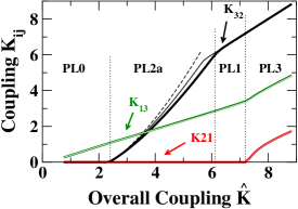
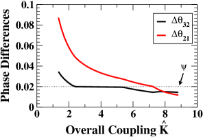
a)   b) c)

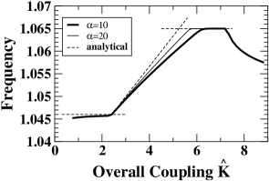
Figure 4: Continuous transitions of the phase-locked state for $N=3$ oscillators. Analytical results are denoted by dashed lines. a) Coupling coefficients $K_{ij}$ as a function of $\hat{K}$. Dotted vertical lines indicate the transitions between different regimes. b) Phase differences. The border of the central region $[-\psi,\psi]$ of the plasticity function is indicated by a dotted line. c) Frequency of the phase-locked state as a function of the overall coupling $\hat{K}$. Parameters: $\alpha=10$ (thick lines) and $\alpha=20$ (thin solid lines), $\tau=100$, $\omega_{1}=1$, $\omega_{2}=1.03$, $\omega_{3}=1.1$, $\tau_{d,p}=0.1$, $\psi=0.02$.

The frequency and coupling coefficients obtained from the perturbation calculation (dashed lines in Fig.4) agree quite well with the numerical simulations (thick solid lines). Nevertheless, for PL2a the differences are quite noticeable. While the upper limit $\alpha$ of the individual synaptic strengths does not appear in the leading-order results (17,19) of the perturbation calculation, it turns out that contributions proportional to $\alpha^{-1}$ arise at next order, which become large for small $\alpha$ (cf. Appendix A). Thus, increasing $\alpha$ from $\alpha=10$ to $\alpha=20$ further improves the agreement (thin solid lines in Fig.4).

Thus, even in this system comprised of only 3 oscillators the combination of the central range $[-\psi,\psi]$ of the plasticity function with the conservation of incoming coupling strengths leads to transitions between at least four regimes in which the phase-locked solution exhibits quite different behavior. As noted before, the transitions between these regimes do not represent bifurcations associated with instabilities but points at which the plasticity function (5) in the underlying differential equations is not differentiable or a coupling strength reaches the maximal value imposed by the weight conservation.

IV Many Oscillators

For larger networks of oscillators an additional, qualitatively different class of stable phase-locked states arises. Sample transition sequences for increasing and for decreasing $\hat{K}$ are shown in Fig.5 for $N=20$ oscillators with frequencies equally spaced in the interval $[1,2]$. In both cases we start with homogeneous coupling, $K_{ij}=\frac{1}{N-1}\hat{K}$, but random phases. For increasing $\hat{K}$ the initial spread in the frequency of the unsynchronized oscillators decreases and step by step the six fastest oscillators merge into a cluster oscillating with a single frequency. At $\hat{K}=29$ all oscillators phase-lock and form a new state, the frequency of which is higher than the natural frequency of the fastest oscillator and increases further with increasing coupling. This new state persists to the largest values of $\hat{K}$ investigated. Decreasing $\hat{K}$ from large values - again starting with homogeneous coupling - a different globally phase-locked state is reached. Its frequency is very close to that of the third fastest oscillator. Near $\hat{K}=50$ it crosses over to a phase-locked state with a frequency very close to that of the second fastest oscillator. At $\hat{K}=40$ that state undergoes a jump transition to the phase-locked state found when increasing $\hat{K}$ from small values.

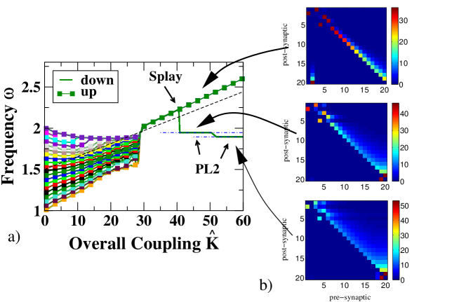
c)   d)

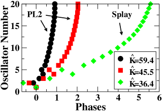
Figure 5: Transitions between three different, globally phase-locked states for $N=20$ oscillators. a) Frequencies as a function of $\hat{K}$. There are two PL2-like states with frequencies close to those of the second- and third-fastest oscillator, respectively, marked by dashed-dotted lines. The analytical result (29) for the splay state is marked by a dashed line. b) Matrices of the coupling coefficients for the two PL2-like states (bottom panels, $\hat{K}=59.4$ and $\hat{K}=45.5$) and the splay state (top panel, $\hat{K}=36.4$). c) Order parameter $r$ as a function of $\hat{K}$ (cf. (20)). It increases with increasing $\hat{K}$ for PL2-like states, but decreases for the splay state. d) Phases of the two near-synchronous PL2-like states and of the splay state. Parameters $\tau=20$, $\tau_{p}=0.15$, $\tau_{d}=0.3$, $\alpha=100$, $\psi=0$.

To understand the main aspects of the phase-locked states consider the coupling coefficients $K_{ij}$ established by the plasticity. With only homosynaptic plasticity each oscillator would be coupled with the maximal strength $\alpha$ to all faster oscillators and would receive no input from any of the slower oscillators. The magnitude of the phase difference between the oscillators would affect only how fast these final values of the coupling coefficients are reached. The heterosynaptic plasticity employed here introduces competition between the incoming couplings and the resulting steady-state values are distributed over the whole range $[0,\hat{K}]$. If $\tau_{p}$ is small the input to each oscillator is predominantly coming from a single other oscillator (Fig.5b). This allows to define chains of dominant coupling. Since the conservation of the overall incoming coupling enforces that each oscillator receives input, these chains must contain loops.

The coexisting phase-locked states differ in characteristic ways in their chains of dominant coupling. Similar to the state PL2 given by (17,19) the states oscillating with frequencies close to those of oscillators 2 and 3, respectively, have strong input from oscillator 2 to oscillator 1 (Fig.5b bottom panels). They differ in additional input from oscillator 3 into oscillators 1 and 2. Although these two coupling coefficients are relatively small, they are sufficient to pull the frequency down to that of oscillator 3. They go to 0 in the cross-over near $\hat{K}=50$. In both states all remaining oscillators receive their dominant input from a single other oscillator, which in most cases is the oscillator with the next higher frequency. Thus, in both states the chain of dominant coupling contains only a small loop involving the fastest oscillators 19 and 20 or 18, 19, and 20, respectively. In the jump transition at $\hat{K}=40$ the input from oscillator 2 into oscillator 1 disappears and instead oscillator 1 receives strong input from the second slowest oscillator (Fig.5b top panel). Consequently, in this state the chain of coupling consists of a single large loop involving essentially all oscillators.

The qualitative difference between the different types of phase-locked states manifests itself also in their phase differences. While in the PL2-like states the phases are closely clustered, the phases of the other state are distributed quite homogeneously over the interval $[0,2\pi]$ (Fig.5d) identifying it as a splay state StMi93 ; SiFa93 ; WaSt94 ; ZoZh09 . The states in the two classes differ therefore significantly in terms of the order parameter

$$r\equiv\frac{1}{N}\left|\sum_{j=1}^{N}e^{i\theta_{j}}\right|,$$ (20)

which characterizes the degree of synchronization of the state. Typically one would expect that the synchronization becomes stronger as the coupling between the oscillators is increased. This is indeed the case for the PL2-type states (Fig.5c). However, in the splay state the order parameter decreases with increasing coupling, indicating that the coupling tends to spread out the phases more uniformly.

IV.1 Perturbation Analysis

To understand the origin of the splay state we again employ a perturbation analysis. It is guided by the observations shown in Fig.5. The characteristic features of the splay state can be captured by considering a regime in which each oscillator interacts only with one other oscillator. This is the case if the window for potentiation $\tau_{p}$ is sufficiently small and the phases are distributed sufficiently homogeneously. Thus, we assume

$$\tau_{p}\ll\min_{1\leq i\leq N}(\Delta\theta_{i+1,i})$$ (21)

and

$$\max_{i}\Delta\theta_{i+1,i}<\min_{i}\Delta\theta_{i+2,i}.$$ (22)

To allow the linearization of the equation of motion for the phases we assume in addition that the number of oscillators is large,

$$N\gg 1,$$ (23)

so that $\Delta\theta_{i+1,i}=\mathcal{O}(N^{-1})$.

This perturbation analysis will be strictly valid in the limit $N\rightarrow\infty$, which implies that all phase differences lie in the central region $[-\psi,\psi]$ of the plasticity function. We expect, however, that this approach will also give good results for intermediate values of $N$ for which $\min_{i}\Delta\theta_{i+1,i}>\psi$. For simplicity we therefore take in this analysis $\psi=0$ with the expectation that the results will also apply to systems with $\psi>0$ as long as $N$ is not too large and therefore $\min_{i}\Delta\theta_{i+1,i}>\psi$.

Here and in the following the phase indices are considered modulo $N$. Thus, in particular, $\Delta\theta_{N,N+1}\equiv\Delta\theta_{N1}$. For the splay state of interest we assume that $\Delta\theta_{N1}-2\pi=\theta_{N}-\theta_{1}-2\pi=\mathcal{O}(1/N)$.

Independent of the assumption (21), $|\Delta\theta_{ij}|>\psi$ implies that for $j<i$ eq.(4) always has a solution $K_{ij}=0$. For $j>i$ the equations (4) for $K_{ij}$ are simplified by the assumptions (21,22), which imply

$$e^{-\frac{1}{\tau_{p}}\Delta\theta_{i+m,i}}\ll e^{-\frac{1}{\tau_{p}}\Delta\theta_{i+1,i}}\quad\mbox{for }m\geq 2.$$ (24)

Thus,

$$\dot{K}_{i,i+m} = \left(\alpha-K_{i,i+m}\right)e^{\frac{1}{\tau_{p}}\Delta\theta_{i,i+m}}-\frac{K_{i,i+m}}{\hat{K}}\left\{-\sum_{j<i}K_{i,j}e^{-\frac{1}{\tau_{d}}\Delta\theta_{i,j}}+\sum_{j>i}\left(\alpha-K_{i,j}\right)e^{\frac{1}{\tau_{p}}\Delta\theta_{i,j}}\right\}$$ (25)

$$= \left(\alpha-K_{i,i+m}\right)e^{\frac{1}{\tau_{p}}\Delta\theta_{i,i+m}}-\frac{K_{i,i+m}}{\hat{K}}\left\{\left(\alpha-K_{i,i+1}\right)e^{\frac{1}{\tau_{p}}\Delta\theta_{i,i+1}}+h.o.t.\right\}.$$ (26)

For $m=1$ the two terms are of the same order and with $\alpha>\hat{K}$ one obtains for the fixed point $K_{i,i+1}=\hat{K}$. For $m\geq 2$ the first term can be neglected relative to the second one due to (24) and one has $K_{i,i+m}=0$. In summary, to leading order the coupling coefficients for the steady state are given by

$$K_{i,i+1} = \hat{K}\qquad i=1,\ldots,N-1,$$

$$K_{N1} = \hat{K},$$ (27)

$$K_{ij} = 0\qquad j\neq i+1,i\neq N.$$

For the phase differences one obtains from (1) for the phase-locked state oscillating with frequency $\omega$

$$\Delta\theta_{i,i+1}=\frac{N}{\hat{K}}\left(\omega_{i}-\omega\right)$$ (28)

to leading order in $\Delta\theta_{i,i+1}$. This direct connection between the phases and the frequencies shows that condition (22) amounts to the assumption that the natural frequencies are not distributed too heterogeneously.

The common frequency $\omega$ of the oscillators is obtained by expressing $\Delta\theta_{N1}$ in two ways. On the one hand one has

$$\Delta\theta_{N1}=\theta_{N}-\theta_{1}=-\sum_{i=1}^{N-1}\Delta\theta_{i,i+1}=-\frac{N}{\hat{K}}\sum_{i=1}^{N-1}\left(\omega_{i}-\omega\right).$$

On the other hand, using $\Delta\theta_{N1}-2\pi=\mathcal{O}(1/N)$ in (3) with $i=N$ yields

$$\Delta\theta_{N1}=2\pi+\frac{N}{\hat{K}}\left(\omega_{N}-\omega\right).$$

Combining the two expressions for $\Delta\theta_{N1}$ results in

$$\omega=\bar{\omega}+2\pi\frac{\hat{K}}{N^{2}}\qquad\mbox{with \qquad}\bar{\omega}=\frac{1}{N}\sum_{i=1}^{N}\omega_{i}.$$ (29)

Replacing $\omega$ in (28) the phase differences are given by

$$\Delta\theta_{i,i+1}=-\frac{2\pi}{N}+\frac{N}{\hat{K}}\left(\omega_{i}-\bar{\omega}\right).$$ (30)

Our analysis assumed $\Delta\theta_{1N}>0$. With (28,29) this implies that the splay state exists only above a minimal coupling strength $\hat{K}_{c}$,

$$\hat{K}>\hat{K}_{c}\equiv\frac{N^{2}}{2\pi}\left(\omega_{N}-\bar{\omega}\right),$$ (31)

and its frequency is above that of the fastest oscillator, $\omega>\omega_{N}$.

Within the framework of (24) small perturbations to the coupling coefficients $K_{ij}$ decouple from the perturbations of the phases $\theta_{i}$ and it is easy to show that the splay state is linearly stable as long as $\alpha>\hat{K}$.

The analytical result (30) shows that with increasing $\hat{K}$ the phases become more evenly distributed, independent of the natural frequencies of the oscillators. This results in a decrease of the order parameter $r$ with increasing $\hat{K}$ in agreement with the numerical simulations (Fig.5b). Eq.(29) captures the linear growth of the oscillation frequency with $\hat{K}$ (dashed lines in Fig.5a). For the parameters of Fig.5a the agreement is, however, not quantitative. In the analytical calculation we considered the limit of small $\tau_{p}$, which allows to assume that each oscillator receives inputs only from a single other oscillator. In Fig.5b this is not quite the case. Reducing the plasticity window to $\tau_{p}=0.05$ with $\tau_{d}=0.1$ yields, however, very good quantitative agreement (Fig.6). Again we find extensive bistability between the splay state and a PL2-like state oscillating with the frequency of the second-fastest oscillator (dash-dotted line). For these parameters we found no transition from the PL2-like state to the splay state when decreasing $\hat{K}$.

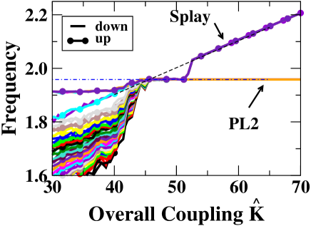
Figure 6: Quantitative agreement of analytical and numerical results for the splay state for $N=25$ oscillators with $\tau_{p}=0.05$ and $\tau_{d}=0.1$. Analytical result (29) denoted by dashed line. Frequency of second-fastest oscillator denoted by dashed-dotted line. Other parameters: $\tau=20$, $\alpha=500$, $\psi=0$.

The fact that the oscillation frequency of the splay state is larger than the natural frequency of the fastest oscillator can be seen to be a direct consequence of the conservation of total incoming weights. It induces an input from the slowest to the fastest oscillator. Since for sufficiently large $N$ the slowest oscillator lags the fastest one by almost $2\pi$, the slowest oscillator is effectively pulling the fastest oscillator ahead.

IV.2 Multiplicity of Attractors

Figs.5,6 show extensive bistability between splay states and PL2-like states. Moreover, Fig.5b,d shows that this splay state does not exactly correspond to the analytically obtained solution since the coupling sequence of oscillators 1 to 6 and with it their firing sequence does not strictly follow their natural frequencies. This suggests that splay states with other firing sequences may exist stably as well.

To investigate the multiplicity of attractors for these larger oscillator networks we have performed simulations with 500 different initial conditions for the phases of the oscillators, keeping the initial coupling coefficients homogeneous, and with different ramping rates for the overall coupling $\hat{K}$. The latter is motivated by the observation that in Figs.5,6 the splay states were obtained by ramping $\hat{K}$ up from small values, while the PL2-like states arose when $\hat{K}$ was set instantly to a value in the phase-locked regime. As expected, the fraction of initial conditions that lead to splay states rather than PL2-like states increases with decreasing ramping rate for $\hat{K}$ (Fig.7).

Figure 7: The fraction of initial conditions leading to splay states rather than PL2-like states decreases with the ramping rate $d\hat{K}/dt$. Parameters: $N=20$, $\hat{K}_{initial}=30$, $\hat{K}_{final}=60$, $\tau_{p}=0.05$, $\tau_{d}=0.1$, $\tau=20$, $\alpha=500$, $\psi=0$.

The splay states reached from the different initial conditions are not all the same. In fact, none of the 267 splay states obtained for $d\hat{K}/dt=0.006$ had the same firing sequence. This is apparent in the firing matrix $\mathbf{F}$ shown in Fig.8a where the color of the element $F_{ij}$ indicates for run $i$ the oscillator that fired at the $j^{th}$-position in the firing sequence. The rows are ordered by the number of the oscillator that fires first, second, third, etc. Analogously, none of the firing sequences of the 233 initial conditions (out of 500) that led to PL2-states appeared twice (Fig.8b).

a)
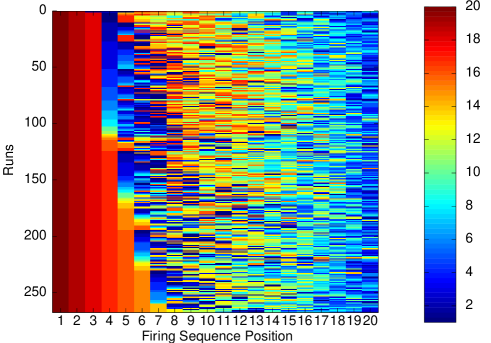
b)

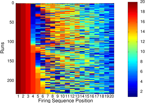
Figure 8: Firing sequences of the states reached using 500 random initial conditions for the phases $\theta_{i}$ but homogeneous values $K_{ij}$. Each row gives the firing sequence for one initial condition. a) 267 splay states. b) 233 PL2-like states. Parameters as in Fig.7, ramping rate $d\hat{K}/dt=0.006$.

Despite their different firing sequences, the various PL2-like states oscillate with a frequency that is extremely close to that of the second-fastest oscillator. This is not the case for the splay states: their frequencies are quite broadly distributed (Fig.9). The difference between the two types of state can be understood intuitively. The PL2 states are dominated by the fastest 2 or 3 oscillators. Different firing sequences of the slower oscillators have therefore little impact on the overall state. In the splay states, however, the fastest oscillator is pulled ahead by one of the slow oscillators, which in turn is pulled ahead by another oscillator and so on until the circle closes with the fastest oscillator pulling a slower one. Since (almost) all oscillators are part of this chain of dominant coupling, the overall state and its frequency depend significantly on the firing order of the slower oscillators.

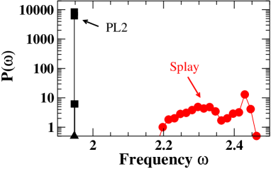
Figure 9: Frequency distribution of splay and PL2-states. The splay states have a broad frequency distribution while the frequencies of the PL2-states are indistinguishable from that of the second fastest oscillator (marked by a triangle). The corresponding firing sequences are shown in Fig.8. Parameters as in Fig.7, ramping rate $d\hat{K}/dt=0.006$.

Can the chain of dominant coupling contain more than a single loop? Fig.10 shows that this is indeed the case. Fig.10a depicts the coupling matrix $K_{ij}$ obtained for one set of initial conditions of the phases with ramping rate $d\hat{K}/dt=0.006$ (cf. Figs.8,9) in which the fastest oscillator $O_{20}$ (marked by a hashed circle in Fig.10b) gets significant input from two slow oscillators, $O_{6}$ and $O_{8}$ (marked by solid circles in Fig.10b). While oscillator $O_{8}$ drives only $O_{20}$, oscillator $O_{6}$ drives in addition also oscillator $O_{1}$, dividing the chain of dominant coupling and generating two loops. The large loop involves all oscillators and reaches eventually $O_{8}$, while the small loop involves only $O_{20-18}$, $O_{7}$, and $O_{6}$. Oscillator $O_{8}$ lags $O_{20}$ by almost $2\pi$ and is therefore effectively pulling $O_{20}$ ahead as in the splay state described above. Oscillator $O_{6}$, however, is only slightly behind $O_{20}$; it actually holds $O_{20}$ back and increases the phase difference between oscillators $O_{8}$ and $O_{20}$ leading to a tighter clustering of the phases of the fastest oscillators $O_{20-18}$.

a)
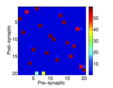
b)

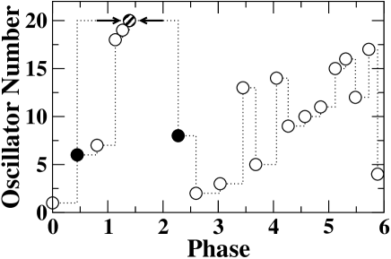
Figure 10: Phase-locked splay state with two loops in the chain of dominant coupling. a) Coupling coefficients $K_{ij}$. Oscillator $O_{20}$ receives input from $O_{6}$ and $O_{8}$. b) Phases of the oscillators with the chain of dominant coupling marked by dotted lines. $O_{6}$ (solid circle) couples to $O_{1}$ and $O_{20}$, holding $O_{20}$ back. Parameters as in Fig.7, ramping rate $d\hat{K}/dt=0.006$.

Fig.11 gives an overview of the splay states shown in Fig.8 in terms of the strengths $K_{20,j}$ of the incoming links of the fastest oscillator $O_{20}$ (Fig.11a) and their frequency (Fig.11b). In the single-loop splay states there is only a single such strong input and it has full strength $\hat{K}$. In the two-loop splay states, however, at least two oscillators provide significant input to $O_{20}$, each with smaller amplitude. With the rows in Fig.11a being sorted by increasing frequency, it is apparent that the bimodal structure of the frequency distribution of the splay states seen in Fig.9 reflects the occurrence of 1-loop and 2-loop states, respectively.

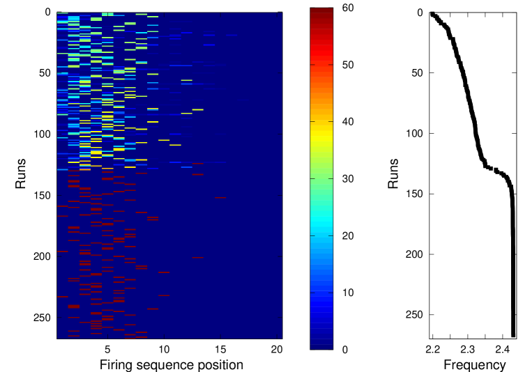
Figure 11: Phase-locked splay states with one and two loops in the chain of dominant coupling. a) Coupling strengths of the incoming links of oscillator $O_{20}$ for the 267 runs resulting in splay states sorted by increasing frequency (cf. Fig.8). Single-loop states have a single incoming link of strength $\sim\hat{K}$, while 2-loop states have multiple, weaker incoming links. b) The frequencies of these states. Parameters: Parameters as in Fig.7, ramping rate $d\hat{K}/dt=0.006$.

Thus, the synaptic competition introduced by the heterosynaptic plasticity combined with the weight conservation stabilizes a variety of splay states with characteristic firing sequences.

V Conclusion

We have investigated the synchronization and phase-locking of networks of weakly coupled oscillators whose interactions evolve in response to the dynamics of the oscillators. Specifically, we considered coupling strengths that are modified slowly depending on the phase difference between the oscillators involved, while keeping the total weight of the incoming connections of any given oscillator constant. This was motivated by observations in neural systems, where spike-timing dependent plasticity is found quite commonly. Our consideration of heterosynaptic plasticity that conserves total incoming weight was triggered by experiments in which the overall strength of all incoming synapses was found to remain approximately constant while individual synapses were potentiated or depressed RoPa03 ; BoHa10 .

For purely homosynaptic plasticity there is only a single state in which all oscillators are phase-locked to each other MaLy07 . In this state each oscillator is coupled equally to all faster oscillators and the overall frequency is that of the fastest oscillator. Including heterosynaptic plasticity with weight conservation, we find a host of different phase-locked states, which fall into two classes: near-synchronous states and splay states.

Due to the continuous transition in the plasticity function between potentiation and depression and due to the conservation of the overall coupling the near-synchronous solutions exhibit quite different behaviors in different parameter regimes. This is reflected in particular in the dependence of the oscillation frequency on the overall coupling strength. For the case of three coupled oscillators we identified various continuous transitions analytically. If the transition region of the plasticity function is narrow the frequency of the near-synchronous solutions depends only weakly on the overall coupling strength. Interestingly, there are large parameter regimes in which the frequency is essentially given by that of one of the oscillators in the network, which is, however, neither the fastest nor the slowest oscillator.

In the splay states the phases are distributed over the whole interval $[0,2\pi]$. A large number of different stable such states are found. In simple splay states the chain of dominant coupling, which represents their effective network structure, forms a single loop and defines a firing sequence characteristic for that splay state. In addition, we also found more complex splay states with a 2-loop structure. A multitude of splay states with different firing sequences coexist stably. Their oscillation frequencies are broadly distributed, reflecting their different firing sequences. Strikingly, the splay states become less synchronized when the coupling strength is increased. At the same time their overall oscillation frequency increases essentially linearly. This frequency is larger than that of the fastest oscillator: the fastest oscillator is pulled ahead by one of the slow oscillators. The essential aspects of the splay states are captured quantitatively in analytical perturbation calculations.

The splay states are characterized by the unidirectional ring topology of their chain of dominant coupling. For fixed, non-plastic coupling strengths the dynamics of oscillators that are coupled unidirectionally in a ring has been studied in detail previously DrCa99 ; CaBu97 ; RoAe04 ; PeYa10 ; PeYa10a ; CaAc10 . Such coupling leads quite naturally to oscillatory states in the form of traveling waves, which correspond to the splay states found here. Results for their stability have been obtained for the Kuramoto model and extensions thereof RoAe04 . For unidirectionally coupled Duffing oscillators their instability has been identified as an Eckhaus instability PeYa10 ; JaPu92 ; KrZi85 . The effect of a delay in the interaction in such networks has also been discussed for an amplitude-equation model and for coupled FitzHugh-Nagumo neurons PeYa10a . For pulse-coupled oscillators the phase-locked solutions have been described using maps for the firing times DrCa99 ; CaBu97 ; CaAc10 . Based on the phase-resetting curves, these analyses showed how the stability of the phase-locked states can be controlled by modifying the phase-resetting curves through slight modifications of the neural dynamics. Thus, in networks functioning as central pattern generators the network dynamics can, for instance, be switched between different animal gaits by injecting a steady current into the neurons DrCa99 ; CaBu97 . These results shed some light on the phase-locked splay states investigated here. However, while in these previous analyses the network structure and the coupling coefficients were kept fixed, an essential part of the dynamics discussed here consists of a restructuring of the chain of dominant couplings.

We have described the network evolution in terms of the self-organization of a network of oscillators with different natural frequencies in the absence of any input. Once established, some of the splay states turn out to persist if all frequencies $\omega_{i}$ are set to the same value, $\omega_{i}=\bar{\omega}$. Thus, eqs.(1,4) can also be read as describing a network of identical neural oscillators that receive heterogeneous tonic input, which modifies their firing rate (natural frequency) and which can be used to train the network to generate different firing sequences. However, due to the sensitive dependence of the firing sequence on the phase distribution of the initial conditions it would be necessary to control also the oscillator phases during the training period to select specific firing sequences.

The focus of this work was the effect of heterosynaptic plasticity on the dynamics of a network of oscillators. In particular, our model has been motivated by the experimental finding that in certain neurons in the amygdala heterosynaptic plasticity roughly balanced homosynaptic plasticity keeping the overall coupling approximately constant RoPa03 ; BoHa10 . In other systems heterosynaptic plasticity may not conserve the overall synaptic weights. Thus, it has been observed that heterosynaptic plasticity can alternatively be controlled by the overall activity of the postsynaptic neuron, independent of its inputs RiMe07 , or that it can reflect limited resources (proteins) of the neuron FoNa04 . In particular in the latter case, it would be natural to model the plasticity by limiting rather than fixing the overall weight of all synapses, as has been done in a model for sequence generation in bird song FiSe10 .

For the description of the oscillators and their interaction we chose a phase model. This is adequate in the limit of weak coupling. The phase model is characterized by its interaction function $H(\Delta\theta)$, which depends on details of the dynamics of the uncoupled oscillators and on their phase-resetting curves HaMa95 ; Er96 . Thus, type-I oscillators, which arise from a saddle-node bifurcation on a circle, and type-II oscillators, which arise from a Hopf bifurcation, typically lead to different functional forms of $H(\Delta\theta)$. Similarly, type-I phase resetting curves, which do not change sign, and type-II phase resetting curves, which do change sign, result in different forms for $H(\Delta\theta)$ . All of the phase-locked states investigated here are characterized by very small phase differences. Therefore only the behavior of $H(\Delta\theta)$ in the immediate vicinity of $\Delta\theta=0$ is relevant for their existence and linear stability. Moreover, due to the conservation of the total incoming weights the constant contribution $H(0)$ can be absorbed into the frequencies of the individual oscillators. The core of our results apply therefore independent of these different types of oscillators and phase resetting curves as long as the interaction is such that the oscillators phase-lock near synchrony when their frequencies are not too different, as is the case in the minimal form of the classic Kuramoto model. Thus, while we were mainly motivated by the dynamics of neural networks, addressing the issue of synchronization and sequential firing, we expect that our results apply to a much larger class of adaptive oscillator networks in the weak coupling regime.

Acknowledgments:

CBP acknowledges financial support from the MICINN (Spain) under project FIS2009-12964-C05-05 and from the FPU program (MEC, Spain). HR gratefully acknowledges support by NSF (DMS-0719944 and DMS-0322807). We thank the referees for critical comments.

Appendix A Higher-Order Expansion for 3 Oscillators

Here we give some more details for the expansion of the solution PL2a to order $\mathcal{O}(\epsilon^{2})$, which reveals the dependence of that solution on $\alpha$ and an additional dependence on $\hat{K}$.

Inserting (6,7,8,9) into the 3 phase equations (3) results at each order in two equations for the phase differences $\delta\theta_{12}^{(1,2)}$ and $\delta\theta_{23}^{(1,2)}$ as well as an equation for one of the individual phases, $\theta_{3}$ say. For phase-locked solutions the latter equation determines the overall frequency of oscillation via $\omega=\dot{\theta}_{3}$. To wit, for PL2a one obtains at $\mathcal{O}(\epsilon)$ (10,11) and

$$\dot{\theta}_{3}=\omega_{1}+\epsilon\left\{\Omega_{3}-\frac{1}{3}\hat{K}\delta\theta_{32}^{(1)}-\frac{1}{3}\left(\hat{K}-K_{32}^{(0)}\right)\delta\theta_{21}^{(1)}\right\},$$

as well as modified equations for $\dot{K}_{ij}^{(0)}$,

$$\tau\dot{K}_{32}^{(0)} = \frac{1}{2}\frac{\alpha}{\Psi\hat{K}}\left(K_{32}^{(0)}-\hat{K}\right)\left(\delta\theta_{32}^{(1)}-\Psi\right),$$ (32)

$$\tau\dot{K}_{21}^{(0)} = -\frac{1}{2}\frac{\alpha}{\Psi\hat{K}}\left(\delta\theta_{32}^{(1)}+\Psi\right)K_{21}^{(0)},$$ (33)

$$\tau\dot{K}_{13}^{(0)} = \frac{\alpha}{\hat{K}}\left(\hat{K}-2K_{13}^{(0)}\right).$$ (34)

The fixed-point solutions of these equations are given by (III) and (17).

To illustrate the form of the contributions at the next order we focus on PL2a. Its fixed-point equations read at $\mathcal{O}(\epsilon^{2})$

$$0 = -\frac{2}{3}\hat{K}\delta\theta_{32}^{(2)}+\frac{2}{3}\frac{3\left(\Omega_{2}-\Omega_{3}\right)+2\hat{K}\Psi}{6\Omega_{2}+\hat{K}\Psi}\delta\theta_{21}^{(2)}+\frac{1}{6}\frac{1}{\hat{K}}\left(6\Omega_{2}+\hat{K}\Psi\right)K_{32}^{(1)}$$

$$+\frac{1}{2}\frac{1}{\hat{K}}\left(2\Omega_{2}+\hat{K}\Psi\right)K_{21}^{(1)}$$

$$0 = \frac{1}{6}\hat{K}\delta\theta_{32}^{(2)}-\frac{1}{3}\hat{K}\delta\theta_{21}^{(2)}-\frac{1}{2}\frac{2\Omega_{2}+\hat{K}\Psi}{\hat{K}}K_{21}^{(1)}-\frac{1}{3}\Psi K_{13}^{(1)}$$

$$0 = \frac{\left(3\left(\Omega_{2}-\Omega_{3}\right)+2\hat{K}\Psi\right)\left(5\Psi^{2}\hat{K}+6\Psi\left(2\Omega_{2}-\Omega_{3}\right)+\alpha\tau_{d}\delta\theta_{32}^{(2)}\right)}{6\Omega_{2}+\Psi\hat{K}},$$

$$0 = K_{21}^{(1)},$$

$$0 = 8\alpha\tau_{p}K_{13}^{(1)}+\hat{K}\Psi\left(2\alpha-\hat{K}\right).$$

Their solution is given by

$$\delta\theta_{32}^{(2)} = -\frac{\Psi}{\alpha\tau_{d}}\left(12\Omega_{2}-6\Omega_{3}+5\hat{K}\Psi\right),$$

$$\delta\theta_{21}^{(2)} = -\frac{1}{2}\frac{\Psi}{\alpha\tau_{d}}\left(12\Omega_{2}-6\Omega_{3}+5\hat{K}\Psi\right)+\frac{1}{8}\frac{\Psi^{2}}{\alpha\tau_{p}}\left(2\alpha-\hat{K}\right),$$

$$K_{32}^{(1)} = -\frac{6\hat{K}^{2}\Psi}{\alpha\tau_{d}}\frac{\left(3\Omega_{2}+\Omega_{3}\right)\left(12\Omega_{2}-6\Omega_{3}+5\hat{K}\Psi\right)}{\left(6\Omega_{2}+\hat{K}\Psi\right)^{2}}-$$

$$\frac{1}{2}\frac{\hat{K}^{2}\Psi^{2}}{\alpha\tau_{p}}\frac{\left(3\left(\Omega_{2}-\Omega_{3}\right)+2\hat{K}\Psi\right)\left(2\alpha-\hat{K}\right)}{\left(6\Omega_{2}+\hat{K}\Psi\right)^{2}},$$

$$K_{21}^{(1)} = 0,$$

$$K_{13}^{(1)} = -\frac{1}{8}\frac{\hat{K}\Psi}{\alpha\tau_{p}}\left(2\alpha-\hat{K}\right).$$

This results in an overall frequency given by

$$\omega=\omega_{1}+\epsilon\left(\Omega_{2}+\hat{K}\Psi\right)-\frac{1}{3}\epsilon^{2}\frac{\hat{K}\Psi}{\alpha\tau_{d}}\left(12\Omega_{2}-6\Omega_{3}+5\hat{K}\Psi\right)+\mathcal{O}(\epsilon^{3}).$$

Thus, the corrections at $\mathcal{O}(\epsilon^{2})$ show that the fixed-point solution is not independent of $\alpha$ as might have been assumed based on the leading-order results. Moreover, the $\alpha$-dependence of the corrections is of $\mathcal{O}(\alpha^{-1})$. Thus, with increasing $\alpha$ the $\mathcal{O}(\epsilon^{2})$-corrections, in particular to the frequency, decrease, consistent with the improved agreement of the perturbation calculation with the numerical simulations seen in Fig.4. Moreover, the phase difference $\Delta\theta_{32}$ for PL2a is not independent of $\hat{K}$ and does not lie exactly at the border of the central region of the plasticity function.

References

- [1] Henry D. I. Abarbanel, R. Huerta, and M. I. Rabinovich. Dynamical model of long-term synaptic plasticity. Proc Natl Acad Sci U S A, 99(15):10132–10137, Jul 2002.
- [2] G.Q. Bi and M.M. Poo. Synaptic modifications in cultured hippocampal neurons: dependence on spike timing, synaptic strength, and postsynaptic cell type. J Neurosci, 18(24):10464–10472, Dec 1998.
- [3] Jennifer N. Bourne and Kristen M. Harris. Coordination of size and number of excitatory and inhibitory synapses results in a balanced structural plasticity along mature hippocampal CA1 dendrites during LTP. Hippocampus, Jan 2010.
- [4] G. Buzsaki and A. Draguhn. Neuronal oscillations in cortical networks. Science, 304(5679):1926–1929, June 2004.
- [5] C. C. Canavier and S. Achuthan. Pulse coupled oscillators and the phase resetting curve. Math.Biosci., 226(2):77–96, August 2010.
- [6] C. C. Canavier, R. J. Butera, R. O. Dror, D. A. Baxter, J. Clark, and J. H. Byrne. Phase response characteristics of model neurons determine which patterns are expressed in a ring circuit model of gait generation. Biol. Cybern., 77(6):367–380, December 1997.
- [7] N. Caporale and Y. Dan. Spike timing-dependent plasticity: a hebbian learning rule. Annu. Rev. Neurosci., 31(2):25–46, August 2008.
- [8] R. Christopher deCharms and Michael M. Merzenich. Primary cortical representation of sounds by the coordination of action-potential timing. Nature, 381(6583):610–613, Jun 1996.
- [9] R. Dror, C. C. Canavier, R. J. Butera, J. W. Clark, and J. H. Byrne. A mathematical criterion based on phase response curves for stability in a ring of coupled oscillators. Biol. Cybern., 80(1):11–23, January 1999.
- [10] B. Ermentrout. Type I membranes, phase resetting curves, and synchrony. Neural Comput., 8(5):979, July 1996.
- [11] I. R. Fiete, W. Senn, C. Z. Wang, and R. H. Hahnloser. Spike-time-dependent plasticity and heterosynaptic competition organize networks to produce long scale-free sequences of neural activity. Neuron, 65(4):563–576, February 2010.
- [12] R. Fonseca, U. V. Nägerl, R. G.M. Morris, and T. Bonhoeffer. Competing for memory: hippocampal LTP under regimes of reduced protein synthesis. Neuron, 44:1011, 2004.
- [13] P. Fries. A mechanism for cognitive dynamics: Neuronal communication through neuronal coherence. Trends Cogn. Sci, 9(10):474–480, October 2005.
- [14] M. Golubitsky, I. Stewart, P. L. Buono, and J. J. Collins. Symmetry in locomotor central pattern generators and animal gaits. Nature, 401(6754):693–695, October 1999.
- [15] J. Guckenheimer and P. Holmes. Nonlinear Oscillations, Dynamical Systems, and Bifurcations of Vector Fields. Springer, 1983.
- [16] D. Hansel, G. Mato, and C. Meunier. Synchrony in excitatory neural networks. Neural Comput., 7(2):307–337, March 1995.
- [17] B. Janiaud, A. Pumir, D. Bensimon, V. Croquette, H. Richter, and L. Kramer. The Eckhaus instability for traveling waves. Physica D, 55:269, 1992.
- [18] J. Karbowski and G. B. Ermentrout. Synchrony arising from a balanced synaptic plasticity in a network of heterogeneous neural oscillators. Phys. Rev. E, 65(3):031902, March 2002.
- [19] L. Kramer and W. Zimmermann. On the Eckhaus instability for spatially periodic patterns. Physica D, 16:221, 1985.
- [20] Y. Kuramoto. Cooperative dynamics of oscillator community - a study based on lattice of rings. Progr. Theor. Phys. Suppl., 79:223, 1984.
- [21] Y. L. Maistrenko, B. Lysyansky, C. Hauptmann, O. Burylko, and P. A. Tass. Multistability in the Kuramoto model with synaptic plasticity. Phys. Rev. E, 75(6):066207, June 2007.
- [22] J. C. Neu. Coupled chemical oscillators. SIAM J. Appl. Math., 37(2):307–315, February 1979.
- [23] P. Perlikowski, S. Yanchuk, O. V. Popovych, and P. A. Tass. Periodic patterns in a ring of delay-coupled oscillators. Phys. Rev. E, 82(3):036208, Sep 2010.
- [24] P. Perlikowski, S. Yanchuk, M. Wolfrum, A. Stefanski, P. Mosiolek, and T. Kapitaniak. Routes to complex dynamics in a ring of unidirectionally coupled systems. Chaos, 20(1):013111, March 2010.
- [25] K. C. Riegle and R. L. Meyer. Rapid homeostatic plasticity in the intact adult visual system. J. Neurosci., 27(39):10556–10567, September 2007.
- [26] J. A. Rogge and D. Aeyels. Stability of phase locking in a ring of unidirectionally coupled oscillators. J. Phys. A, 37(46):11135–11148, November 2004.
- [27] S. Royer and D. Pare. Conservation of total synaptic weight through balanced synaptic depression and potentiation. Nature, 422(6931):518–522, April 2003.
- [28] A. T. Schaefer, K. Angelo, H. Spors, and T. W. Margrie. Neuronal oscillations enhance stimulus discrimination by ensuring action potential precision. PLoS Biology, 4(6):E163, June 2006.
- [29] R. Sepulchre, D. Paley, and N. Leonard. Collective motion and oscillator synchronization. Cooperative Control, 309:189–205, 2005.
- [30] M. Silber, L. Fabiny, and K. Wiesenfeld. Stability results for in-phase and splay-phase states of solid-state laser arrays. J. Opt. Soc. Am. B, 10(6):1121–1129, June 1993.
- [31] S. H. Strogatz. From Kuramoto to Crawford: Exploring the onset of synchronization in populations of coupled oscillators. Physica D, 143(1-4):1–20, September 2000.
- [32] S. H. Strogatz and R. E. Mirollo. Splay states in globally coupled josephson arrays - analytical prediction of floquet multipliers. Phys. Rev. E, 47(1):220–227, January 1993.
- [33] E. Vaadia, I. Haalman, M. Abeles, H. Bergman, Y. Prut, H. Slovin, and A. Aertsen. Dynamics of neuronal interactions in monkey cortex in relation to behavioral events. Nature, 373(6514):515–518, February 1995.
- [34] S. Watanabe and S. H. Strogatz. Constants of motion for superconducting Josephson arrays. Physica D, 74(3-4):197–253, July 1994.
- [35] L. P. Zhu, Y. C. Lai, F. C. Hoppensteadt, and J. P. He. Cooperation of spike timing-dependent and heterosynaptic plasticities in neural networks: a Fokker-Planck approach. Chaos, 16(2):023105, June 2006.
- [36] W. Zou and M. Zhan. Splay states in a ring of coupled oscillators: From local to global coupling. SIAM J. Appl. Dyn. Sys., 8(3):1324–1340, December 2009.